Article

A Hybrid Algorithm for Short-Term Wind Power Prediction

1
School of Computer and Electronic Information, Guangxi University, Nanning 530004, China
2
Guangxi Key Laboratory of Multimedia Communications and Network Technology, Nanning 530004, China
3
Dispatch and Control Center of Guangxi Power Grid, Nanning 530023, China
*
Author to whom correspondence should be addressed.
Energies 2022, 15(19), 7314; https://doi.org/10.3390/en15197314
Submission received: 6 September 2022 / Revised: 27 September 2022 / Accepted: 30 September 2022 / Published: 5 October 2022
(This article belongs to the Special Issue Emerging Technologies and Methods for Future Energy Markets)

Abstract

:
Accurate and effective wind power prediction plays an important role in wind power generation, distribution, and management. Inthis paper, a hybrid algorithm based on gradient descent and meta-heuristic optimization is designed to improve the accuracy of prediction and reduce the computational burden. The hybrid algorithm includes three steps: in the first step, we use the gradient descent algorithm to get the initial parameters. Secondly, we input the initial parameters into the meta-heuristic optimization algorithm to search for the “best parameters” (high-quality inferior solutions). Finally, we input optimized parameters into the RMSProp optimization algorithm and conduct gradient descent again to find a better solution. We used 2021 wind power data from Guangxi, China for the experiment. The results show that the hybrid prediction algorithm has better performance than the traditional Back Propagation (BP) in accuracy, stability, and efficiency.

1. Introduction

In the 21st century, with the rapid economic development, the world’s demand for energy is growing. As traditional energy sources can no longer satisfy the needs of green economic development, a consensus among countries has emerged on how to reduce carbon emissions and develop renewable energy. Among renewable energy, wind power is widely concerned and rapidly developing due to its advantages of non-pollution, renewable and relatively mature utilization technology. Wind power has evolved into the most mature power generation technology among all renewable energy sources as time has passed [1]. According to the Global Wind Energy Council (GWEC), 2020 is a record year for the global wind power industry, with a global installed capacity of 93 GW, a year-on-year increase of 53%. China and the United States are already the two largest wind energy markets in the world [2]. However, wind energy also faces unavoidable problems. The inherent randomness, volatility, and intermittent power generation may seriously impact the grid system. Wind power prediction is important to reduce grid dispatching costs and improve system performance. Wind power prediction is divided into three classes based on the time scale: long-term, medium-term, and short-term. Long-term forecasting is for wind farm planning and annual power generation plans, and medium-term forecasting is utilized to make a weekly or monthly maintenance plan. These two prediction algorithms have less accuracy, and less study has been done in this field [3]. On the other hand, short-term forecasts are for the next few minutes to a few hours. They can aid in frequency regulation, rotating reserve capacity, and cost-effective load dispatch, making them a popular topic in the wind energy business. As a result, the majority of recent research has concentrated on predicting short time series of wind power generation.
The mainstream wind power forecasting methods nowadays can be divided into four categories: physical analysis method, statistical analysis method, machine learning methods, and the combined methods [4,5,6,7]. Among them, the physical analysis method is based on numerical weather prediction (NWP) and geographic terrain information to obtain current wind speed and wind direction data at the hub height of the wind turbine, and then calculate the output power based on the wind turbine power feature curve [8] to establish the wind power forecasting model. This method has the advantage of not relying on historical data, but the complex calculation model leads to its poor performance in real-time or short-term tasks [9,10,11], and the numerical weather forecast accuracy and update frequency can affect the forecast accuracy and speed [12].
In contrast to physical analysis, the statistical method only requires past wind speed data. The wind power prediction model is established using pattern recognition and parameter estimation. Many wind speed prediction models and wind power prediction models have been proposed using statistical methods, such as the moving average model [13], Markov model [14], and Bayesian model [15] et al. In conclusion, short-term wind power forecasting can be accomplished using statistical methods that can develop an ideal link between predicted wind power and historical data. However, it has to require a large number of historical samples with the same trend to construct an accurate model [16].
The statistical analysis method, which uses historical wind speed data as a single input, ignores the strong nonlinearity of wind power data, while the machine learning method considers the relationship between the output and multiple variables. The overall trend also shows that the machine learning method is more accurate [17]. Under the condition of sufficient historical samples, it usually has high prediction accuracy and strong generalization ability. Moreover, machine learning method has a lot of different machine learning models, including ANN model [18], support vector machine (SVM) model [19], BPNN model [20], and extreme learning machines (ELM) model [21], et al. They have been utilized for wind power prediction or wind speed prediction. Among them, the results of SVM and neural networks have been satisfactory in terms of prediction [22]. Ning and Liu utilized the particle swarm algorithm to optimize the penalty factor and kernel parameters of SVM and then used historical data as training samples to train the optimized SVM model [23]. On the other hand Liu and Wang proposed a short-term forecasting model of BPNN with the combined loss function for wind power generation [24]. Kassa et al. [25] proposed a hybrid GA-BP neural network wind power generation prediction method. However, these popular methods also have some problems. Firstly, the training time of SVM is too long, and it is very difficult to realize large-scale training samples; Secondly, BPNN is a gradient attenuation (GD) optimization algorithm [26]. Although the convergence speed is fast, the disadvantage of using the GD algorithm is that they converge easily to the local minimum value and it is sensitive to the initial value of parameters. Because the problem is not a convex programming problem, the local minimum is not the global optimal solution [27]. Instead of using the BP approach to calculate the neural network parameters, we may utilize a meta-heuristic optimization algorithm to solve this problem. Meta-heuristic algorithm does not ensure that the best solution can be found, as discussed in [28], they can, nevertheless, come up with high-quality inferior solutions. The proposed SFLA-ANN in [29] is found to be more accurate than the traditional BPNN and GA-ANN, but SFLA also has its unavoidable problem, SFLA will bring a lot of computational burdens. Therefore, in [30], BP will be used to find the initial parameters of SFLA, then through optimization to obtain better parameters, these parameters have faster convergence and higher accuracy than SFLA-ANN. However, the BP-SFLA-ANN algorithm [30] only discusses the possibility of prediction in short-term solar energy, and it ignores the crucial point that after the sub-optimal parameters obtained by SFLA, further optimization can still be sought by gradient descent. In the theory we have just described, BP enables the algorithm to find an optimum faster, but it gets stuck in a local optimum, whereas SFLA enables the algorithm to provide a certain amount of randomness that allows it to jump out of the local optimum. Can we assume that after SFLA we perform a fast gradient descent optimization algorithm to get better parameters?
In this paper, to resolve these problems, we need to reasonably use SFLA and BP. Therefore a new hybrid algorithm model (i.e., BP-SFLA-RMSprop-ANN) is proposed to achieve better performance, and we will discuss the reliability of BP-SFLA-RMSprop-ANN and whether it can be applied in short-term wind power prediction. The remainder of this paper is as follows: The proposed forecasting algorithm theory and its implementation are in Section 2. The simulation results and discussion are in Section 3. Finally, in Section 4, the conclusions are presented.

2. Algorithm Theories

2.1. Shuffled Frog Leaping Algorithm

SFLA is a meta-heuristic search algorithm that simulates the memetic evolution of a group of hungry frogs. The algorithm’s concept is based on the behavior of a group of frogs who live in a swamp with numerous stones. These frogs’ ultimate goal is to discover the place with the most food. To find and arrive at this, the frogs communicate with each other while searching, allowing them to enhance each other’s places in the swamp. We can find the SFLA combines two completely different logics, “certainty” and “randomness” to simulate communication and realize SFLA. Through the deterministic strategy, frogs only care about their local improvement. In the random strategy, all frogs in the swamp complete the global information exchange and use a flexible random model to avoid converging to the local minimum. The algorithm is divided into three primary steps, which are as follows:
  • Classification process: In this step, we want to obtain different class frogs (as frogs in the same class, we will use them for local search in the next step). To this end, frogs should be sorted according to their fitness values (training error), and then the sorted first set member, that is, the best frog in the swamp should be placed in the first memeplex, the second frog in the second memeplex, the M frog in the M memeplex (M = the numbers of memeplexes), the (M + 1) frog in the first memeplex, and so on.
  • Local search process: In this step, the worst frog in each memeplex communicates with the best frog in each memeplex and adjusts the frog’s leaping step and direction to increase its fitness value. During each iteration, this step will be repeated some times (epochs). The equations explaining this step are expressed in (1) and (2):
    D = rand ( ) · X b X w , old
    X w , new = X w , old + D ; D max D D max
    where X b , X w , old , and X w , new respectively represent the location of the local best frog in each class, the current worst frog in each class, and the generated new frog. D and D max represent the transition step size and the maximum transition step size, respectively. Rand () represents a positive random value between 0 and 1. It will take the place of the old frog if it is more fit than previously. Otherwise, this operation will be repeated for this frog. The difference is that this time, the global best frog ( X g , b ) will be compared instead of the best local ( X b ). Equation (3):
    D = rand ( ) · X g , b X w , old
    If this strategy still does not produce better fitness values for frogs, then we will make the frog (the local worst frog) jump randomly once in the solution space. In each epoch, each frog jumps at least once and at most three times in each generation. After the epoch is completed, it is necessary to calculate the fitness value of local frogs (i.e., frogs in the same memeplex) to determine the current local best and worst frogs in the memeplex.
  • Shuffling process: After each repetition, each iteration, all frogs are integrated together.
These three operations will be repeated as different iterations of SFLA until they meet the requirements and stop running. Figure 1 shows the flowchart of SFLA. More details about the concept of the hybrid algorithm and its implementation will be described in detail later.

2.2. BP-SFLA-RMSprop-ANN Model

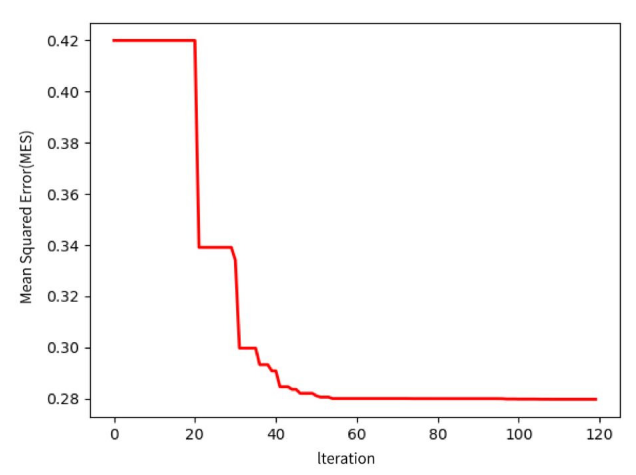
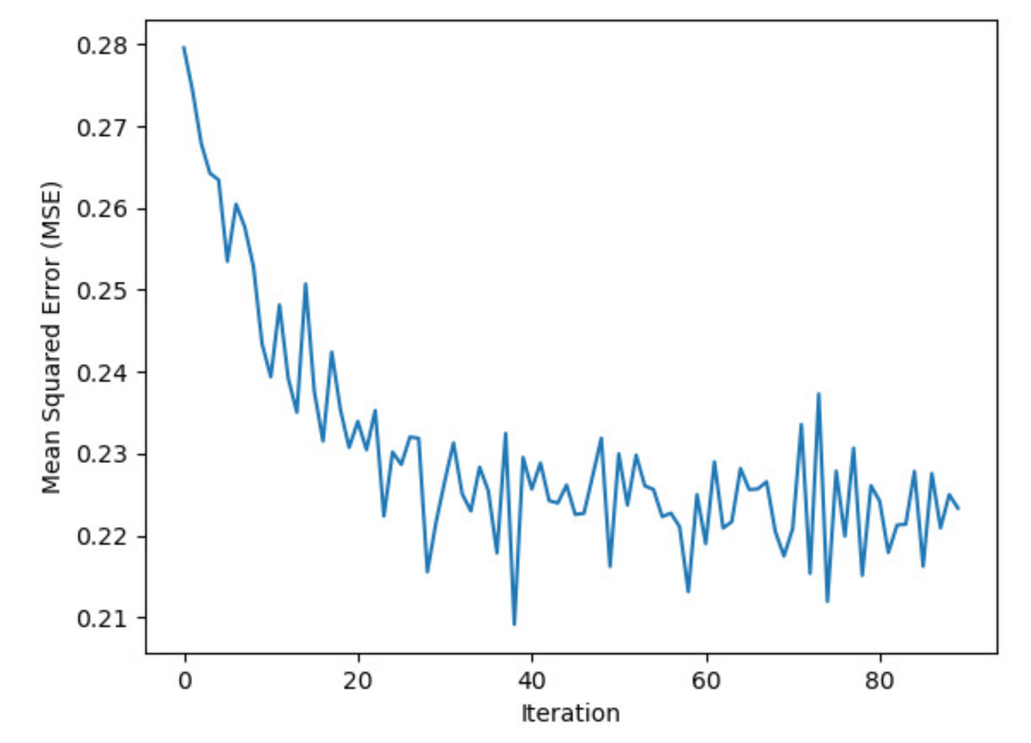
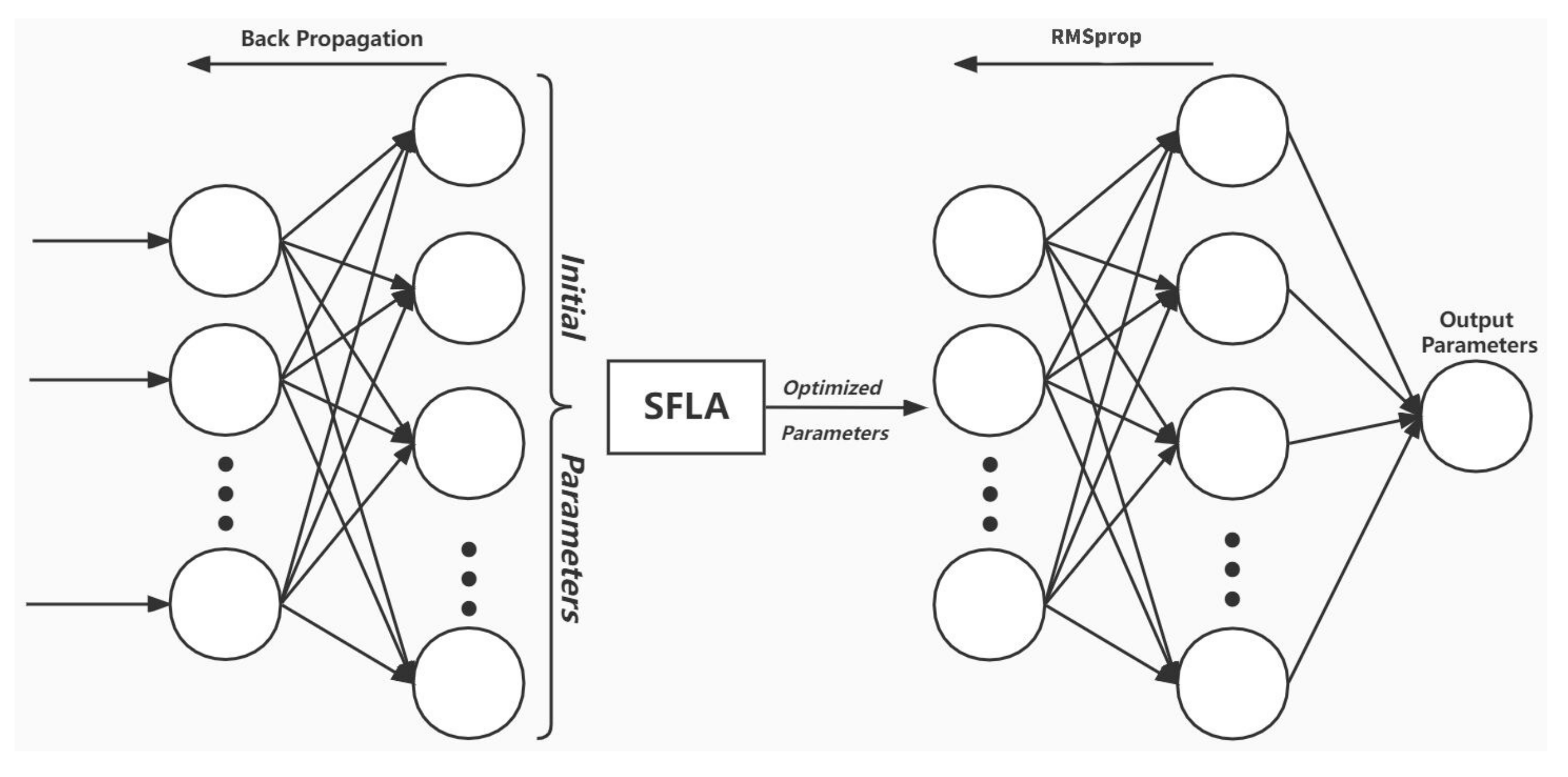
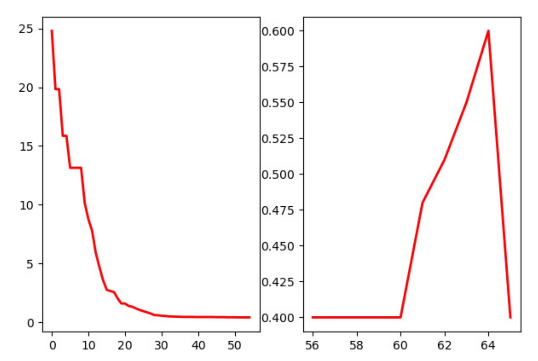
The logic of the hybrid prediction model proposed in this paper adopts meta-heuristic algorithm (SFLA) to adjust the parameters of typical feedforward ANN. While using the SFLA, we do not give up using the classical BP algorithm. This algorithm first provides high-quality initial parameters for the SFLA and prevents the meta-heuristic algorithm from starting the search process from too random areas (that is, the advantages of this algorithm compared with the model proposed in [29]), and in [30], the parameters optimized by SFLA are directly input into ANN to start predicting. However, this model (i.e., BP-SFLA-ANN) ignores the drawback of the “randomness” strategy in SFLA. When the number of SFLA’s iterations reaches a certain number, subsequent iterations will be hard to effectively optimize the parameters. As shown in Figure 2, the number of iterations of SFLA reaches more than 50, its training error will not decrease. So in the last step, the parameters obtained from SFLA should be optimized by RMSprop algorithm again (RMSprop is more purposeful than SFLA and faster than classic BP), Figure 3 well demonstrates that using RMSprop for parameter optimization in the second half can make the training error show a fluctuating downward trend. The minimum value in this trend is the parameter we need. Figure 4 shows a structure diagram of the model. Firstly, the weights and biases in BPNN are used to form the initial frog population. The number of frogs, memeplexes, iterations, epochs (local search iterations), and the maximum jumping distance of frog individuals are set; Secondly optimization is carried out until the defined convergence conditions are met. Finally, the parameters obtained by SFLA are optimized by RMSprop. The new algorithm is verified by combined with training and test samples. The specific steps are as follows:
  • BPNN initialization. Set the structure of the BPNN, design the number of neurons in each layer, and initialize the weights and biases.
  • SFLA parameter initialization. We set the number of frogs, memeplexes, iterations, and epochs in the algorithm.
  • Calculate the fitness value. The initial parameters obtained by the BP algorithm are used as the initial frog population.
  • Perform the classification step in the SFLA mentioned above.
  • Perform the local search step in the SFLA mentioned above.
  • Perform the shuffling step in the SFLA mentioned above.
  • If the maximum number of iterations is satisfied, the optimal solution is output, otherwise, return to step 4.
  • Optimized again. The optimal parameters input into RMSprop and they will be optimized again.
  • Verify the algorithm. After the training, diagnose the test samples, analyze the results and verify them.

2.3. Overfitting

In the training process of neural networks, we need to solve the overfitting problem. ANN is based on its prediction performance to change its prediction efficiency, and its training goal is to minimize training error. Therefore, if the training process does not stop at the correct point, it will start to “remember” the training samples rather than “summarize” the training samples. In this paper, cross validation [31] will be used to solve this problem. The data set is divided into three subsets: training set, test set, and validation set. While training with available training samples, ANN compares the error of the training set with the error of the validation set after each iteration. If the validation error continues to increase by a certain number (the threshold is set as five times in this paper), the training process will stop immediately, and the solution with “minimum validation error” will be used to predict.

3. Case Study

3.1. Wind Speed Data Description

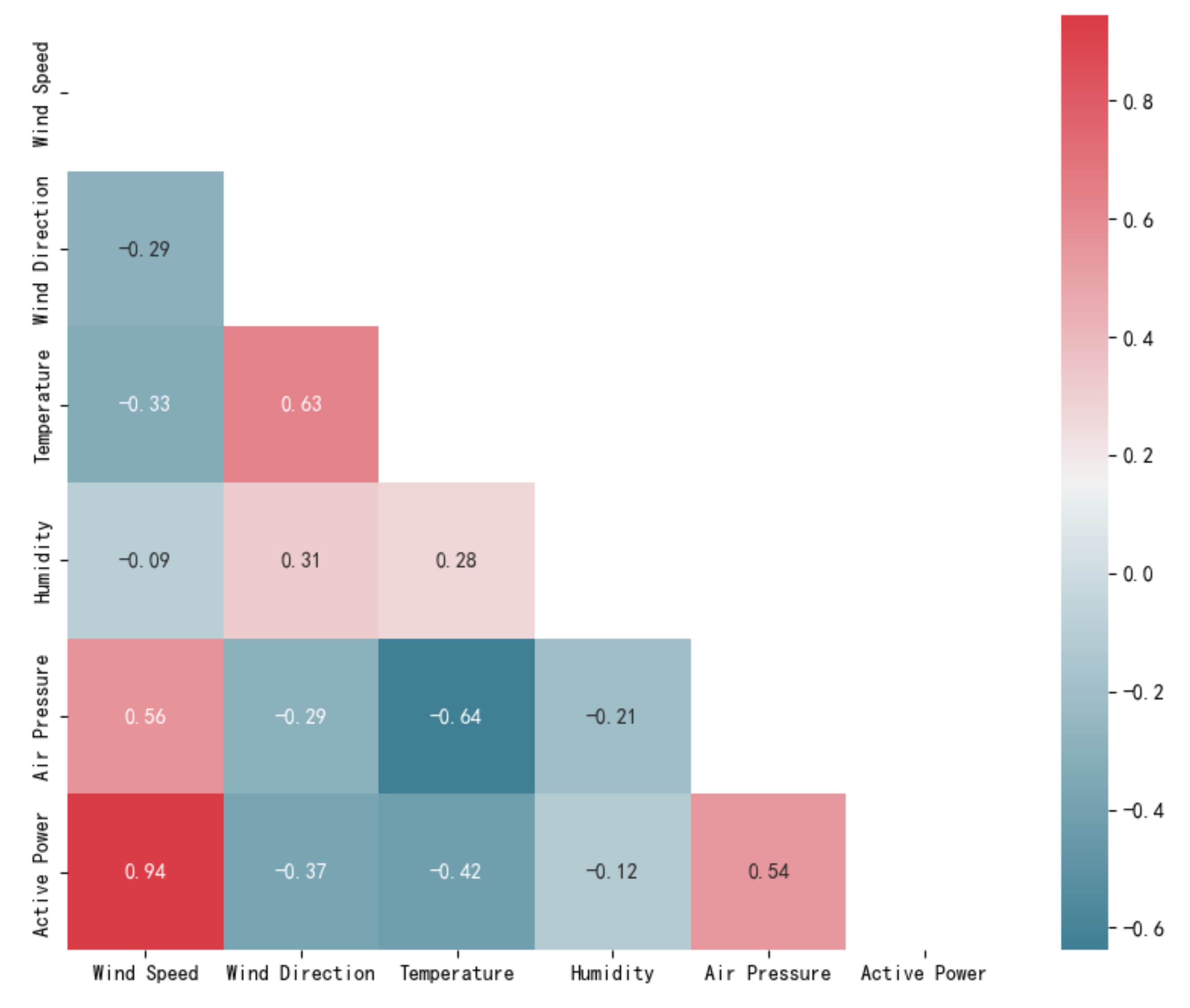
The wind power data sets are provided by China Southern Power Grid. The data sets record wind speed (m/s), wind direction (°), temperature (°C), humidity (RH), air pressure (HPA) and active power (MW) of the wind turbine in the past year. Each measurement interval is 15 min, and there are 52,429 sets of valid data in these wind farms. The data of the first five groups are shown in Table 1, and Figure 5 shows the correlation between the individual data features, we should ensure that the absolute value of the correlation of the data features for model training must be higher than the threshold (i.e., it is set 0.1 in this paper).
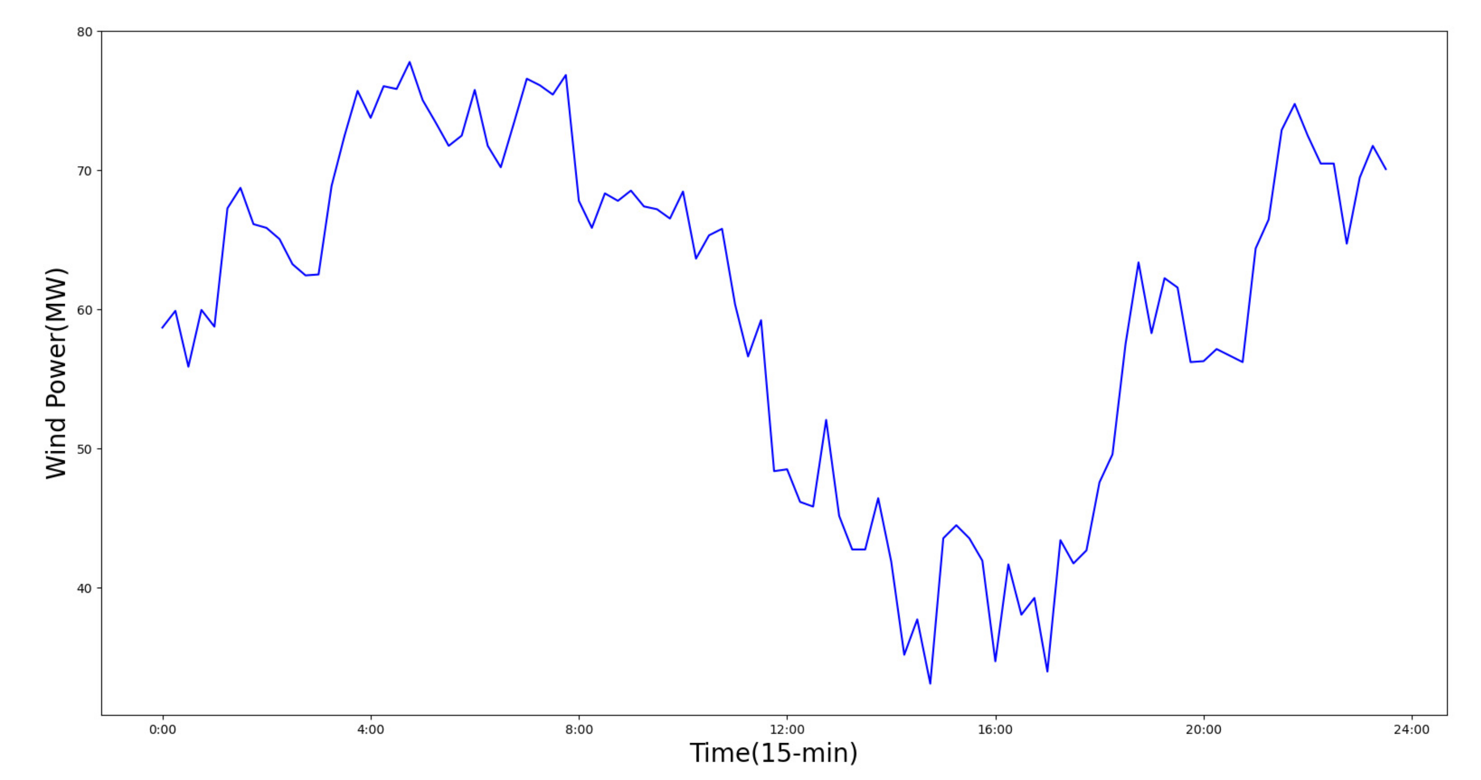
Although the presented model is forecasting the short-term wind power data (i.e., 5-min, 10-min, 15-min, …, 25-min, and 30-min), the optimization-prediction process will be repeated dozens of times to cover various types of changes in wind power output in a day or a week. The daily data must be sufficiently detailed to ensure model training, testing, and validation, Figure 6 depicts the someday wind power trend.

3.2. Data Process

Wind speed, wind direction, temperature, humidity and air pressure are used as the features, and wind power is used as output data. Firstly, we need to eliminate outliers in the data set. Secondly, in order to solve the problem of overfitting, through cross validation, the data set is divided into three parts: training set, test set and validation set to realize model construction, performance evaluation and parameter optimization respectively, with a ratio of 5:2.5:2.5. We employ min-max normalization to handle the data in order to increase prediction accuracy and speed up model optimization. The normalization function is to scale the data to [0, 1], the formula is:
x k = x k x min x max x min

3.3. Simulation Results

We study the SFLA to optimize the weights and biases of BPNN. We set the number of frogs, memeplexes, iterations and epochs in the SFLA to 30, 3, 100 and 10 respectively. Then we use mean squared error (MSE), mean absolute error (MAE), mean absolute percentage error (MAPE) and R 2 as evaluation criteria. The calculation formulas are:
MSE = 1 N i = 1 N pretict i test i 2
MAE = 1 N i = 1 N predict i test i
MAPE = 100 % n i = 1 n test i predict i test i
R 2 = 1 i test i predict i 2 i test ¯ i test i 2
We will acquire 30 training errors after each training process. The best training error of each iteration is the output value. Figure 7a illustrates the downward trend of the best training error. In order to clarify the continuous reduction of the loss function in the presentation optimization process, we describe three different intervals during 0–100 iterations. b, c, and d in Figure 7 describe the decreasing trend of training error of 0–30 iterations, 30–60 iterations, and 60–100 iterations respectively.
To avoid overfitting, the threshold is set to five times. If the validation error continues to rise for five times, the training process will stop. In Figure 8, we can observe this problem occurs when iteration is #60, this is why the training does not reach its maximum number of iterations (i.e., Iteration #100) and stops right at the #65.
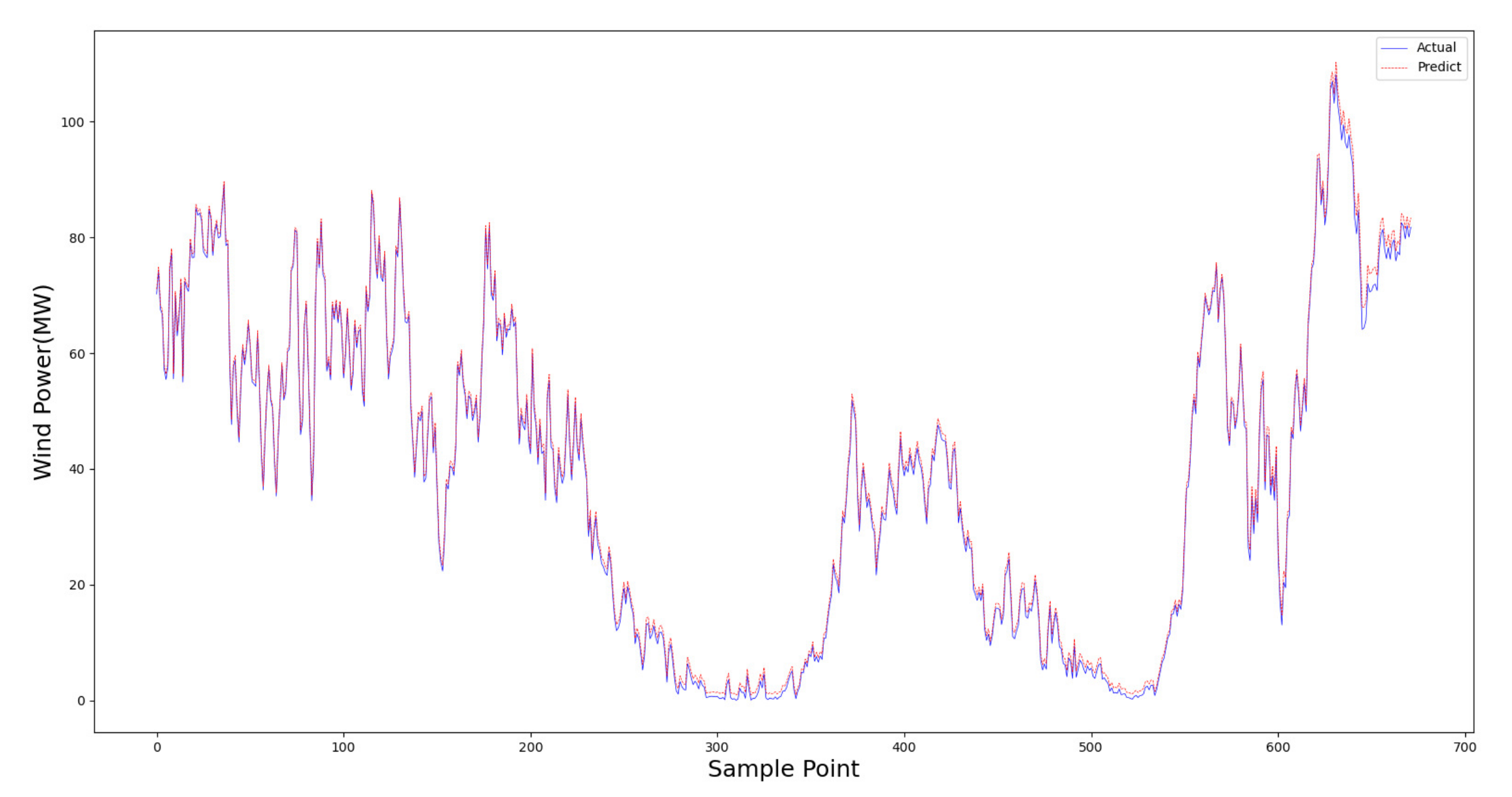
Despite the proposed algorithm focusing on short-term wind power forecasting, the optimization-forecasting process will be performed six times per week to account for different oscillations. Figure 9 shows the results of comparing the predicted wind power data with the actual data for the test week of 1 July to 7 July.
In the comparison experiments, we selected two similar models (i.e., BP-ANN, BP-SFLA-ANN) and two classical models (i.e., LSTM [32], GRU [33]) to compare with the proposed model. All models are in the same circumstances, with the same number of iterations, the same learning rate, and the same division of data to evaluate the efficiency of the proposed models. Furthermore, we use seconds to unify their running time units for easy comparison. Table 2 presents the performance and time-consuming comparison among the proposed model, BP-ANN, BP-SFLA-ANN, LSTM, and GRU. As shown in the Table, the proposed hybrid method delivers the best accurate prediction and the second shortest running time. With the same number of iterations, the RMSprop algorithm can effectively improve the accuracy and reduce the high running time brought by the shuffled frog leaping algorithm. It successfully proves that the theory is feasible.

4. Conclusions

Accurate, efficient, and reliable wind power prediction can greatly help power plants to carry out distribution management. The paper innovatively proposes a hybrid algorithm-based meta-heuristic optimization method and gradient descent algorithm. In this paper, the BPNN is firstly used to determine the initial parameters of SFLA. Then the SFLA is used to optimize its initial parameters, which are finally fed back to the RMSprop for further convergence. The algorithm has three advantages: 1. High-quality random initial parameters are obtained quickly from the BP algorithm. 2. Combines the strategies of randomness and determinism from the frog-hopping algorithm. 3. Go through RMSprop for a fast descent gradient. The proposed BP-SFLA-RMSprop-ANN in this paper predicts short-term wind power in the Guangxi province of China. The simulation results show that the algorithm’s prediction performance is the best among these similar algorithms, and it has a good convergence speed. In future work, we intend to optimize the algorithm further to improve convergence speed and prediction performance. To make it more suitable for the application of short-term wind power forecasting.

Author Contributions

Conceptualization, Z.X.; methodology, Z.X.; software, Z.X. and G.B.; validation, Z.X., G.B. and Y.C.; investigation, Y.Z. and K.H.; data curation, Y.Z. and K.H.; writing—original draft preparation, Z.X.; writing—review and editing, Z.X. and Y.C.; visualization, Z.X. and G.B.; supervision, Y.C.; project administration, Y.C.; funding acquisition, Y.C. All authors have read and agreed to the published version of the manuscript.

Funding

This research was funded by the Natural Science Foundation of Guangxi Province OF FUNDER grant number 2020GXNSFAA159090.

Data Availability Statement

Available online: https://github.com/cookiecase/Hybrid-algorithm (accessed on 20 July 2022).

Conflicts of Interest

The authors declare no conflict of interest.

Abbreviations

The following abbreviations are used in this manuscript:
SFLAShuffled frog leaping algorithm
RMSPropRoot mean square propagation
ANNArtificial neural network
BPBack propagation
NWPNumerical weather prediction
SVMSupport vector machine
ELMExtreme learning machines
GDGradient descent
MSEMean squared error
MAEMean absolute error
MAPEMean absolute percentage error
LSTMLong short-term memory
GRUGated recurrent unit

References

  1. Yuan, X.; Chen, C.; Yuan, Y.; Huang, Y.; Tan, Q. Short-term wind power prediction based on LSSVM–GSA model. Energy Convers. Manag. 2015, 101, 393–401. [Google Scholar] [CrossRef]
  2. Global Wind Energy Council. GWEC| Global Wind Report 2021; Global Wind Energy Council: Brussels, Belgium, 2021. [Google Scholar]
  3. Kanna, B.; Singh, S.N. Long term wind power forecast using adaptive wavelet neural network. In Proceedings of the 2016 IEEE Uttar Pradesh Section International Conference on Electrical, Computer and Electronics Engineering (UPCON), Varanasi, India, 9–11 December 2016; pp. 671–676. [Google Scholar]
  4. Wang, H.Z.; Li, G.Q.; Wang, G.B.; Peng, J.C.; Jiang, H.; Liu, Y.T. Deep learning based ensemble approach for probabilistic wind power forecasting. Appl. Energy 2017, 188, 56–70. [Google Scholar] [CrossRef]
  5. Huang, N.; Wu, Y.; Cai, G.; Zhu, H.; Yu, C.; Jiang, L.; Zhang, Y.; Zhang, J.; Xing, E. Short-term wind speed forecast with low loss of information based on feature generation of OSVD. IEEE Access 2019, 7, 81027–81046. [Google Scholar] [CrossRef]
  6. Guo, T.; Zhang, L.; Liu, Z.; Wang, J. A combined strategy for wind speed forecasting using data preprocessing and weight coefficients optimization calculation. IEEE Access 2020, 8, 33039–33059. [Google Scholar] [CrossRef]
  7. Wang, H.; Lei, Z.; Zhang, X.; Zhou, B.; Peng, J. A review of deep learning for renewable energy forecasting. Energy Convers. Manag. 2019, 198, 111799. [Google Scholar] [CrossRef]
  8. Yining, W.; Da, X.; Xitian, W.; Guojie, L.; Miao, Z.; Zhang, Y. Prediction of interaction between grid and wind farms based on PCA-LSTM model. Proc. CSEE 2019, 14, 4070–4081. [Google Scholar]
  9. Zhao, J.; Guo, Z.H.; Su, Z.Y.; Zhao, Z.Y.; Xiao, X.; Liu, F. An improved multi-step forecasting model based on WRF ensembles and creative fuzzy systems for wind speed. Appl. Energy 2016, 162, 808–826. [Google Scholar] [CrossRef]
  10. Wu, B.; Song, M.; Chen, K.; He, Z.; Zhang, X. Wind power prediction system for wind farm based on auto regressive statistical model and physical model. J. Renew. Sustain. Energy 2014, 6, 013101. [Google Scholar] [CrossRef]
  11. Haque, A.U.; Nehrir, M.H.; Mandal, P. A hybrid intelligent model for deterministic and quantile regression approach for probabilistic wind power forecasting. IEEE Trans. Power Syst. 2014, 29, 1663–1672. [Google Scholar] [CrossRef]
  12. Feng, S.; Wang, W.S.; Liu, C.; Dai, H. Study on the physical approach to wind power prediction. Proc. CSEE 2010, 30, 1–6. [Google Scholar]
  13. Singh, P.K.; Singh, N.; Negi, R. Short-term wind power prediction using hybrid auto regressive integrated moving average model and dynamic particle swarm optimization. Int. J. Cogn. Inform. Nat. Intell. (IJCINI) 2021, 15, 111–138. [Google Scholar] [CrossRef]
  14. Song, Z.; Jiang, Y.; Zhang, Z. Short-term wind speed forecasting with Markov-switching model. Appl. Energy 2014, 130, 103–112. [Google Scholar] [CrossRef]
  15. Li, X.; Wu, J.; Xu, Z.; Liu, K.; Yu, J.; Guan, X. Uncertainty Set Prediction of Aggregated Wind Power Generation based on Bayesian LSTM and Spatio-Temporal Analysis. In Proceedings of the 2021 IEEE 17th International Conference on Automation Science and Engineering (CASE), Lyon, France, 23–27 August 2021; pp. 361–366. [Google Scholar]
  16. Li, L.; Liu, Y.Q.; Yang, Y.P.; Shuang, H.; Wang, Y.M. A physical approach of the short-term wind power prediction based on CFD pre-calculated flow fields. J. Hydrodyn. Ser. B 2013, 25, 56–61. [Google Scholar] [CrossRef]
  17. Ahmed, A.; Khalid, M. A review on the selected applications of forecasting models in renewable power systems. Renew. Sustain. Energy Rev. 2019, 100, 9–21. [Google Scholar] [CrossRef]
  18. Peiris, A.T.; Jayasinghe, J.; Rathnayake, U. Forecasting wind power generation using artificial neural network:“Pawan Danawi”—A case study from Sri Lanka. J. Electr. Comput. Eng. 2021, 2021, 5577547. [Google Scholar] [CrossRef]
  19. Wang, S.; Chen, C. Short-Term Wind Power Prediction Based on DBSCAN Clustering and Support Vector Machine Regression. In Proceedings of the 2020 5th International Conference on Computer and Communication Systems (ICCCS), Shanghai, China, 15–18 May 2020; pp. 941–945. [Google Scholar]
  20. Peng, G.; Cun, W. Wind Power Prediction Based on Back Propagation Algorithm with Numerical Weather Prediction. In Proceedings of the 2019 7th International Conference on Information Technology: IoT and Smart City, Shanghai, China, 20–23 December 2019; pp. 468–471. [Google Scholar]
  21. Luo, X.; Sun, J.; Wang, L.; Wang, W.; Zhao, W.; Wu, J.; Wang, J.H.; Zhang, Z. Short-term wind speed forecasting via stacked extreme learning machine with generalized correntropy. IEEE Trans. Ind. Inform. 2018, 14, 4963–4971. [Google Scholar] [CrossRef] [Green Version]
  22. Tan, L.; Han, J.; Zhang, H. Ultra-short-term wind power prediction by salp swarm algorithm-based optimizing extreme learning machine. IEEE Access 2020, 8, 44470–44484. [Google Scholar] [CrossRef]
  23. Lu, N.; Liu, Y. Application of support vector machine model in wind power prediction based on particle swarm optimization. Discret. Contin. Dyn. Syst. S 2015, 8, 1267. [Google Scholar] [CrossRef]
  24. Liu, F.; Wang, Z.; Liu, R.D.; Wang, K. Short-term forecasting method of wind power generation based on BP neural network with combined loss function. J. Zhejiang Univ. 2021, 55, 594–600. [Google Scholar]
  25. Kassa, Y.; Zhang, J.; Zheng, D.; Wei, D. A GA-BP hybrid algorithm based ANN model for wind power prediction. In Proceedings of the 2016 IEEE Smart Energy Grid Engineering (SEGE), Oshawa, ON, Canada, 21–24 August 2016; pp. 158–163. [Google Scholar]
  26. Christodoulou, C.; Georgiopoulos, M. Applications of Neural Networks in Electromagnetics; Artech House, Inc.: Norwood, MA, USA, 2000. [Google Scholar]
  27. Yang, L.; Luo, J.; Xu, Y.; Zhang, Z.; Dong, Z. A distributed dual consensus ADMM based on partition for DC-DOPF with carbon emission trading. IEEE Trans. Ind. Inform. 2019, 16, 1858–1872. [Google Scholar] [CrossRef]
  28. Schmidt, H.P.; Ida, N.; Kagan, N.; Guaraldo, J.C. Fast reconfiguration of distribution systems considering loss minimization. IEEE Trans. Power Syst. 2005, 20, 1311–1319. [Google Scholar] [CrossRef]
  29. Asrari, A.; Ramos, B. An intelligent neural network-based short-term wind power forecasting in PJM electricity market. In Proceedings of the 2016 IEEE Power and Energy Society General Meeting (PESGM), Boston, MA, USA, 17–21 July 2016; pp. 1–5. [Google Scholar]
  30. Asrari, A.; Wu, T.X.; Ramos, B. A hybrid algorithm for short-term solar power prediction—Sunshine state case study. IEEE Trans. Sustain. Energy 2016, 8, 582–591. [Google Scholar] [CrossRef]
  31. Pindoriya, N.; Singh, S.; Singh, S. An adaptive wavelet neural network-based energy price forecasting in electricity markets. IEEE Trans. Power Syst. 2008, 23, 1423–1432. [Google Scholar] [CrossRef]
  32. Li, J.; Geng, D.; Zhang, P.; Meng, X.; Liang, Z.; Fan, G. Ultra-Short Term Wind Power Forecasting Based on LSTM Neural Network. In Proceedings of the 2019 IEEE 3rd International Electrical and Energy Conference (CIEEC), Beijing, China, 7–9 September 2019; pp. 1815–1818. [Google Scholar]
  33. Xu, Z.; Yixian, W.; Yunlong, C.; Xueting, C.; Lei, G. Short-term Wind Speed Prediction Based on GRU. In Proceedings of the 2019 IEEE Sustainable Power and Energy Conference (iSPEC), Beijing, China, 21–23 November 2019; pp. 882–887. [Google Scholar]
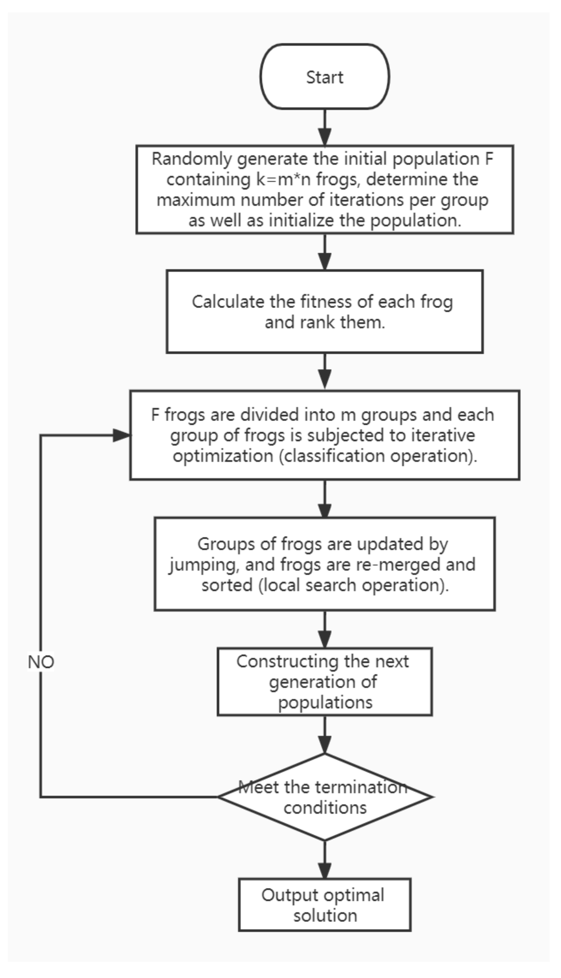
Figure 1. Flowchart of the shuffled frog leaping algorithm.
Energies 15 07314 g001
Figure 2. Training error of SFLA.
Energies 15 07314 g002
Figure 3. Training error in the second half using RMSprop.
Energies 15 07314 g003
Figure 4. Structure diagram of the proposed model.
Energies 15 07314 g004
Figure 5. Heat map of feature correlation.
Energies 15 07314 g005
Figure 6. Wind power trend in someday.
Energies 15 07314 g006
Figure 7. Training error (x-axis: Iteration; y-axis: MSE (%)).
Energies 15 07314 g007
Figure 8. Validation error (x-axis: Iteration; y-axis: MSE (%)).
Energies 15 07314 g008
Figure 9. The wind power prediction of the test week.
Energies 15 07314 g009
Table 1. The dataset’s first five groups of data.
SampleWind Speed (m/s)Wind Direction (°)Temperature (°C)Humidity (RH)Air Pressure (HPA)Active Power
(MW)
15.3541.5216.5185.41964.9420.36
25.0641.4416.6084.58965.1920.36
34.8239.8016.9782.49965.3616.28
45.0125.6716.5084.01966.2516.88
54.1556.5018.6485.00965.399.31
Table 2. The comparison of similar algorithms.
Prediction ModelsPerformance Metrics
MSEMAEMAPE R 2 Run Time (s)
Hybrid Algorithm(BP-SFLA-RMSprop-ANN)0.37540.408318.41%0.9539107
BP-ANN0.83610.753632.63%0.910687
BP-SFLA-ANN0.52760.507922.13%0.9374136
LSTM1.17080.785438.86%0.8834206
GRU1.59040.921646.75%0.8547146
Publisher’s Note: MDPI stays neutral with regard to jurisdictional claims in published maps and institutional affiliations.