Article

Challenges in Kinetic Parameter Determination for Wheat Straw Pyrolysis

1
Institute of Catalysis Research and Technology (IKFT), Karlsruhe Institute of Technology (KIT), Hermann-von-Helmholtz-Platz 1, Building 727, 76344 Eggenstein-Leopoldshafen, Germany
2
Institute of Thermal Engineering, Graz University of Technology, Inffeldgasse 25b, 8010 Graz, Austria
3
Thermal and Fluids Engineering Department, Carlos III University of Madrid, Avda. de la Universidad 30, Leganés, 28911 Madrid, Spain
*
Author to whom correspondence should be addressed.
Energies 2022, 15(19), 7240; https://doi.org/10.3390/en15197240
Submission received: 22 August 2022 / Revised: 19 September 2022 / Accepted: 23 September 2022 / Published: 1 October 2022
(This article belongs to the Topic New Advances in Waste and Biomass Valorization)

Abstract

:

Highlights

  • Second-derivative (DDTG) curves helped overcome the challenges of overlapping peaks in the DTG curves of wheat straw;
  • Deconvolution methods lead to high errors in the estimation of lignin content;
  • Curve-fitting methods lead to lower errors when determining the kinetics of biomass degradation, especially for hemicellulose;
  • Reaction networks were modified to consider K content to describe straw pyrolysis.

Abstract

Wheat straw is a renewable agricultural by-product that is currently underutilized in the production of bioenergy and bioproducts due to its high ash content, as well as high transport costs due to its low volumetric energy density. The thermogravimetric analysis of this material produces derivative curves with a single broad peak, making it difficult to identify the three conventional pseudo-components (cellulose, hemicellulose, and lignin), which is resolved using the second derivative to determine inflection points. Model-fitting methods and isoconversional methods were applied to determine the degradation kinetics of wheat straw at two different particle sizes, as well as that of a reference feedstock (beech wood), and the obtained values were used to divide the degradation curves to be compared to the experimental data. Seven different pyrolysis reaction networks from the literature were given a similar treatment to determine which provides the best estimation of the actual pyrolysis process for the case of the feedstocks under study. The impact of the potassium content in the feedstock was considered by comparing the original pathway with a modification dependent on the experimental potassium content and an estimated optimum value.

1. Introduction

As a thermochemical conversion method, the detailed and complex mechanism of pyrolysis remains unknown, though current models have simplified it into a set of competitive and consecutive reactions of the main pseudo-components cellulose, hemicellulose, and lignin. It is important to keep in mind that pyrolysis is also a step in the combustion and gasification processes, hence enhancing the importance of understanding the fundamentals. Despite being unable to reproduce the heating rates observed in a fast pyrolysis process, thermogravimetric analysis (TGA) is still the state-of-the-art means of determining kinetic parameters for this degradation method [1].
It is very common to determine pyrolysis kinetics or degradation pathways using TGA, which determines the variation of mass loss over time. The repeatability of this method is often low, a fact attributed to heterogeneity within a sample batch and phenomena such as thermal lag [2].
Experimental results for TGA analysis of biomass are abundant in the literature, and several reviews and comparisons have been published. Among these, White et al. [3] condensed many different sources while providing a comprehensive explanation of the available methods for deriving degradation kinetics from TGA data. On the other hand, Anca-Couce et al. [4] provided a graphical analysis of the dispersion of some previously published results.
The main methods of processing TGA data for the assessment of kinetic data are through model-fitting or the use of so-called isoconversional methods [5]. The latter were devised to obtain the variation of Arrhenius parameters with the extent of conversion. In contrast to the model-fitting methods that consider the whole weight loss, isoconversional methods allow for the estimation of parameters for specific conversion values. Depending on the assumptions made, there are several methods available, the applicability and methodology of which have been very well discussed by Cai et al. [5].
A common method of comparing the efficacy of prediction methods for kinetics is through their activation energy, which quantifies the minimum amount of energy that must be provided for a system to result in a chemical reaction, and is represented in formal units of energy/mol (e.g., kJ·mol−1) [6]. Wu et al. [7] established the relationships between the effective activation energies, obtained as a function of the conversion using the isoconversional methods, and the different stages of the degradation of biomass. The authors performed the study on tobacco waste, which contains compounds such as pectin and nicotine, which do not play a part in most lignocellulosic materials’ degradation. The authors proposed the division of the DTG curve into a series of ranges that divide the weight loss profile into regions and disregard the concurrence of degradation of different pseudo-components (PCs), akin to what was proposed by Sher et al. [8]. On the other hand, this logic also fails by considering the decomposition of lignin as occurring after the temperature at which the curve flattens (transition between the active and passive pyrolysis zones), where exothermic charring reactions dominate [9], and may not be completely attributed to lignin degradation but also secondary pyrolysis.
However, in the case of wheat straw and several other lignocellulosic biomasses, the distinction between the hemicellulose and cellulose peaks is difficult, as already pointed out by Šimkovic and Csomorová [10]. The second derivative of the mass loss (henceforth named DDTG) can be used to estimate the point corresponding to a hemicellulose peak based on the fact that the cellulose degradation often happens within a smaller range of temperatures during TGA and corresponds to the period of maximum degradation rate (the highest DTG peak). The degradation of hemicellulose happens over a larger range of temperatures, as reflected in a separate lower peak or a shoulder/bump at temperatures below the maximum degradation temperature. This shoulder/bump corresponds to the progressive lowering of the DDTG until a minimum, after which the cellulose degradation dominates, which is visible in the DTG curve as the peak of a small shoulder [9,11]. This minimum is taken as the hemicellulose point, as shown by Gaitán-Álvarez et al. [11], who noticed a similar issue with biomasses such as Tectona grandis.
The determination of the lignin peak is a contentious topic when using TGA data to determine the kinetics and/or lignocellulose composition. On the one hand, the decomposition range is reported to cover the whole range of a typical TGA run, meaning that its presence will affect the results obtained for the other two pseudo-components by representing an underlying curve that affects the performance of curve-fitting methods. Most sources use the end-point of the cellulose degradation, where a visible change in the slope of the DTG is observable, as the point of maximum degradation of lignin is therefore the center of the pseudo-component degradation curve. However, this is a contentious topic, as the area of DTG typically corresponding to lignin can also be influenced by charring processes at high temperatures. On the other hand, the decomposition of lignin is a complex process that should not be described using a single reaction, as the decomposition is commonly represented by three [12,13] or even seven pseudo-monomers [14], which decompose at different temperatures. Regardless, this process is often modeled with a single component.
It must be kept in mind that values for temperature ranges for the different lignocellulosic components in the literature are often non-consensual, especially in the case of lignin, for which values may range from 250 to 500 °C [15], or even span the entire degradation range, as far as 900 °C [16].
Multicomponent model-fitting makes use of the simultaneous degradation of multiple pseudo-components to estimate the kinetic parameters that describe the degradation of biomass [1,2,4]. While more complex than considering the biomass as a single component, it often leads to better fits for biomasses whose degradation has several stages (represented as peaks/shoulders in the DTG profile) [1,4,17,18,19].
Reaction networks were developed to predict the degradation of lignocellulosic biomasses and product distribution [2]. The current state of the art seems to be a competitive and concurrent mechanism for the degradation of the different lignocellulosic components developed by the Ranzi group at the CRECK Modeling Group at the Politecnico di Milano, Italy [12]. The model is comprised of complete detailed reaction networks, including kinetic parameters. Since 2008, the model was improved by several authors by modifying the kinetic parameters and/or the product distribution [20], the inclusion of a radical mechanism for the degradation of lignin [14], the inclusion of pyrolysis of plant extractives, and triglycerides [21,22,23] considering different types of hemicellulose [21,22,23] or the extent of charring during the pyrolysis process [13]. Pecha et al. [24] compiled a very thorough review of the historical development of pyrolysis reaction modeling from cellulose-focused to detailed kinetic models which include possible products and intermediates.
The majority of these models were developed from the thermogravimetric data of the isolated lignocellulosic fractions, and therefore did not take into account the catalytic effect of alkali metals within the ash, which are known to reduce oil yields and alter product composition [2,25]; however, Trendewicz et al. [26] published a modified cellulose degradation network with activation energy which is a function of the potassium fraction in the feedstock. To the best of the authors’ knowledge, the application of the reaction networks for ash-rich plant biomasses, such as wheat straw, has not been evaluated to date.
Thermogravimetry is most often performed with small sample sizes and particle sizes to minimize buoyancy effects and heat/mass diffusional limitation effects, however, no studies were found by the authors which compared the effect of particle size during TGA for the case of wheat straw. Marcilla et al. [27] tested the effects of particle size on the thermal degradation of both almond shells and olive stones using this method decrease in particle sizes was shown to lead to a lower solid residue yield and a higher rate of convolution between the hemicellulose and cellulose peaks, which may be attributed to the higher ash contents in finer sieves, leading to a reduction in the temperature of the cellulose peak.
The known effects of particle sizes were studied several times in the past. It is a known fact that pyrolysis setups with very small particles and very low vapor residence times lead to high bio-oil yields by mitigating secondary reactions [28,29]. Wang et al. [30] showed that the variation in the diameter of wood cylinders has a minor effect on the liquid yield, but thicker cylinders lead to a higher water production. Shen et al. [31] proposed that the mechanical particle size reduction (shredding, milling) leads to higher oil yields due to disruption of the internal particle structure, leveling out after a certain particle size. This fact was corroborated by Salehi et al. [32], who noticed a decrease of 10% in bio-oil yield when increasing the sieve fraction from <0.59 mm to 0.59–1 mm for higher fractions. Decreases in coal yield with a lower particle size were found by Demirbaş [33] using olive husks and Luangkiattikhun et al. [34] using oil palm solid waste, while Pütün et al. [35] found no correlation for sunflower pressed bagasse, in contrast to coal and oil shales.
According to Anca-Couce et al. [4], in an analysis of 17 sources using different methods, the activation energy for each pseudo-component shows a substantial variance, and was the highest for cellulose (75–250 kJ/mol), followed by hemicellulose (55–200 kJ/mol), and then lignin (15–215 kJ/mol).
Lopéz [36] (Table 1) analyzed wheat straw similar to that presented in this manuscript and performed the succinct analysis of different kinetic determination methods using TGA. However, the authors considered a lower range of conversion values and a higher range of temperatures, as well as analyzed the kinetic parameters without considering the different lignocellulosic fractions.
A series of literature values for wheat straw are presented in Table 2, and the values associated with the isolated fractions of wheat straw are presented in Table 3. Of these, the Coats–Redfern method (as well as the unrecognized method) cannot be compared with those obtained in the context of this work, as they are based on degradation using a single heating rate, often leading to the activation energy values of a lower order of magnitude. Additionally, several authors omitted the pre-exponential factor in the published results.
A kinetic model is required to improve the process modeling, which often disregards the presence of ash in biomasses. The objective of this work was to obtain reliable kinetic data for the pyrolysis of biomass with a high ash content, such as, e.g., wheat straw, which are not available yet. Thermogravimetry is a widely used experimental method to obtain kinetic parameters for pyrolysis, however, in order to do so, two major challenges need to be addressed to acquire reliable kinetic data for biomass with a high ash content. First, one single peak is observed during the thermogravimetry of high-ash feedstock (such as wheat straw) due to the catalytic effects of inorganic compounds present in the feedstock. This observation demands a reproducible method to deconvolute such single peaks into three, one for each of the main biomass macromolecular components—cellulose, hemicellulose, and lignin. Secondly, the available reaction schemes for pyrolysis were derived from feedstocks with relatively low ash contents and it follows that validation is required as to whether they can be applied to an ash-rich feedstock due to the aforementioned catalytic effects.
The objective was met by testing the use of the DDTG evaluation of the experimental TGA data from wheat straw, representing a high ash content feedstock. The results were compared to experimental TGA data from beech wood, representing a low ash content feedstock, to evaluate the impact of the ash content. These experimental datasets were compared with simulated data computed using kinetic parameters from previously published biomass pyrolysis reaction networks.

2. Materials and Methods

In the context of this report, the thermogravimetry data of wheat straw at two different particle sizes were analyzed. Wheat straw powder (WS-P) and not-pulverized wheat straw (≈5 mm, WS-H, from ‘hull’). The thermogravimetric data of beech wood powder (beech) which were previously presented in another publication [4] were used as a comparison feedstock due to its lower ash content.
Wheat straw (Triticum aestivum L.) was procured from a local farmer (Dörrmann, Kraichtal-Münzesheim, Germany), supplied in spring wheat bales (250–300 kg). The straw was shredded to a particle size of <5 mm using a disintegrator (HZR 1300) and cutting mill (LM 450/1000-S5-2) delivered and installed by ‘Neue Herbold Maschinen- und Anlagenbau GmbH’ (Sinsheim/Reihen, Germany). Beech wood was supplied for a round-robin test, the details of which can be found in Anca-Couce et al. [4].

2.1. Analytic Methods

The elementary analysis of the biomass samples was performed according to the DIN EN 15,104 standard. The elementary characterization of the inorganic ash fraction of biomass was performed using a variation of the DIN EN ISO 21,587 standard. Inductively coupled plasma optical emission spectroscopy (ICP-OES) was performed using an Agilent 725 spectrometer coupled with a simultaneous echelle spectrometer with radial plasma observation. Argon was employed as both plasma gas (15 L/min, excitation at 40 MHz, and 2 KW) and auxiliary gas (1.5 L/min). Samples were dissolved in hydrofluoric acid (HF) and analyzed using a feed rate of 1.3 mL/min, for a total of 3 measurements over 8 s. Before the measurement, each sample was dissolved in an acid mixture: HNO3 (65%), HCl (37%), HF (40%), H2O2 (35%), on a prepared glass beak. The analysis of the feedstocks can be found in Table 4.
For tests with particles of low dimensions, a SPEX SamplePrep Freezer-Mill 6875 was employed to powder samples of up to 10 g, using 2–3 cycles of 10 min (precool 5 min, 3 cycles of 1 min grinding, 1 min cool time, at a rate of 10 cps) to a particle size of approximately 100 mesh (149 μm).

2.2. Thermogravimetry

The TGA data were obtained in-house using a Netzsch STA-409 thermal analysis system at the following linear heating rates: 1, 5, 10, and 20 K·min−1 up to 900 °C. The WS-P and WS-H samples were submitted to all these heating rates as well as 50 K·min−1. The software is able to export mass loss data as a function of time or temperature, as well as compute the first and second derivatives of these curves. The 10 K·min−1 WS-P was submitted to 5 replicas (initial mass 224.2 ± 11.0 mg) to estimate the measurement error during TGA, leading to an error of 0.31% for the maximum degradation rate temperature (DTG peak), 0.00% for the solid residue yield, and 0.25% for the maximum degradation rate value. The analysis of all samples can be found in Supplementary Information (SI).

2.3. Data Analysis

The analysis of the system was restricted to the temperature range of 150–500 °C, according to the methodology used by Anca-Couce [1,4], limiting the number of points to 250. The second mass-loss derivative was employed to estimate the points of the maximum degradation of each lignocellulosic pseudo-component (an example of which is shown in Figure 1). This method was employed for every set of thermogravimetric data.
The estimations of the temperatures and conversion points for the maximum degradation of each pseudo-component were performed by analyzing the inflection points of the second derivative curve (DDTG), for which the hemicellulosic peak center is determined by the minimum of the DDTG, the cellulose peak corresponds to a zero of the curve at which DDTG becomes positive, and the lignin peak to the inflection point where the DDTG curve flattens at approximately 0. (Figure 1) This method is based on the strategy employed by Gaitán-Álvarez et al. [11]. The software-mediated numerical estimation of the second derivative, such as that employed in the context of this manuscript, features an error proportional to the square of the step size (O(h2)), where h refers to the temperature step. A description of the mathematical proof can be found at [47].
After estimating the temperatures and conversion points for the maximum degradation of each pseudo-component, it is possible to apply Voigtian deconvolution methods to estimate the lignocellulosic content of the biomass, assuming a dry-ash-free basis. This logic is an adaptation of the method employed by Rego et al. [48], and the lignocellulosic relative distribution is based on the ratio of the areas of the curves. The software employed was the Origin Pro 2019, and the employed curves were Gaussians. The standard error reported is the error in the area determination divided by the value of the said area.
The kinetic parameters of the TGA data may be estimated in several ways, however, the most common are model-fitting and isoconversional methods. Both methods make use of material conversion (α, Equation (1), where m0 stands for the initial mass, m stands for the current mass, and mf for the final mass) [1].
α = 1 m m f m 0 m f
Multicomponent model-fitting makes use of summative Arrhenius curves of the form described in Equation (1), for which A stands for the pre-exponential factor and Ea for the activation energy for each pseudo-component i, if it fits. The position and shape of the accrued pseudo-component curves are very sensitive to either of these parameters. These methods employ pseudo-components, which are assumed to represent the three lignocellulosic polymers: cellulose, hemicellulose, and lignin. These degrade simultaneously and non-competitively (Equation (2), where ci and αi stand for the relative fraction and conversion of each pseudo-component i), and their degradations are represented by Arrhenius kinetics (Equation (3)) [1].
d α d t = i = 1 n c i d α i d t
d α i d t = A i exp E a , i R T f α i
The conversion function, f(α) (Equation (4)), is commonly assumed to be first-order (n = 1). Şen et al. [49] also considered the contracting-sphere (n = 2/3) and three-halves (n = 3/2) models. Manyà et al. [17] reported interesting results when employing n = 3 for the degradation of Kraft lignin, and Gomèz [18,19] reported better results when using these results when modeling the degradation of different lignocellulosic biomasses. Anca-Couce et al. reported better values when leaving the order of the reaction as a fitting parameter with good results to better account for the variability of the curve shape with the specifications of each biomass [1,4].
f α i = 1 α i n
The method used to model-fit the experimental data was based on that employed by Anca-Couce [1], in that the fit is simultaneous for all DTG curves of a material, normalized using the lowest value (-DTG peak). The fit was based on the least-squares minimization of the objective function (Equation (5)) over N = 250 experimental points, using a GRG nonlinear solver (bundled with Microsoft Excel™ 2016). The quality of the fit was evaluated using Equation (6) (root sum of square errors), normalized using the difference between the peak and the minimum experimental derivatives of conversion. The fit for each case was taken to be the average of the results of each DTG curve.
S = i = 1 N d α i d t e x p d α i d t s i m 2
f i t % = S N d α i d t e x p ,   m a x d α i d t e x p ,   m i n
Cai et al. [5] discussed the problems concerning the numerical estimation of the derivative of the conversion at each point, as proposed in the method presented in Equation (7), where t may stand for either time or temperature.
d α i d t i = α i + 1 α i t i + 1 t i   for   the   start   point 1 2 α i α i 1 t i t i 1 + 1 2 α i + 1 α i t i + 1 t i for   intermediate   points α i α i 1 t i t i 1 for   the   end   point
In this study, three isoconversional methods were employed: the Flynn–Wall–Ozawa (FWO) method (Equation (8)), the Kissinger–Akahira–Sunose (KAS) method (Equation (9), and the Friedman differential method (Equation (10)), based on the methodology presented by Cai et al. [5] and Carrier et al. [50], and demonstrated by Vyazovkin et al. [51] (where βi represents the apparent heating rate (ΔT/Δt)). The Kissinger method (Equation (11)) is used to estimate kinetic parameters at a maximum degradation rate (Tmax), and its results are presented in the SI.
ln β i = 1.052 E α R T α , i + ln A α E α ln 1 α R 5.331 .
ln β i T α , i 2 = E α R T α , i + ln A α R ln 1 α E α
ln β i d α d T α , i = E α R T α , i + ln A α 1 α
ln β T max 2 = ln A R E a E a , max R T max
Using isoconversional methods, the kinetic parameters are determined using linear regression, with the energy of activation equaling the slope of the fit, and the pre-exponential factor being a function of the intercept. The results were estimated in intervals of α 0.05, and were disregarded at high conversions due to a large error. These methods are often employed due to their ease of applicability and comparable results; in addition, due to making use of data at different heating rates, it may be feasible to employ them at high heating rates for which kinetic determination is unpractical.
The peak associated with each pseudo-component and feedstock changes with the heating rate; therefore, the average of the kinetic parameters corresponding to each lignocellulosic fraction was calculated based on the peak conversions determined by the second derivative method. For each conversion value, the kinetic parameters were determined considering the distance to the closest multiple of α 0.05 (e.g., for a peak conversion of 0.37, the value is estimated by taking 3/5 of the α 0.35 value and 2/5 of the α 0.4 value).
The deviation (ε, root sum of square errors, results are best when approaching zero) was estimated as shown in Equation (12). The mass loss comparison (TGA) was performed against the experimental 1 − α curves to disregard the presence of residual solid content, and the derivative mass loss (DTG) was compared to the experimental dα/dt curves for consistency. For the case of DTG-based comparisons, (1 − α)exp is replaced by the (dα/dt)exp curve at time i:
ε = R S S E = i = 1 N 1 α e x p , i 1 α k i n , i 2 N

2.4. Simulation of Mass Loss Curves

The simulation of the mass loss curves for the purpose of being compared with experimental TGA data was performed using spreadsheet software (in this case, Microsoft Excel™ 2016) based on the method employed by Anca-Couce et al. for MatLab™ [1].
The method makes use of the temperature time stamps of experimental TGA data (beech straw powder, heating rate of 10 K·min−1). For each temperature T, the derivative of the mass loss of a solid component αi was estimated using Equation (3) and using n = 1 when estimating f(α) (Equation (4)). The mass loss curves were computed by numerical integration using the forward Euler method, with time steps given by the timestamps on the original thermogravimetric data (Equation (13)). This method features a local error of (O(h)), for which h refers to the time step [52]. The value of (1 − αi) at time 0 is defined as 1 for the components present at time 0, and 10−5 for those absent.
1 α i t = j = 1 α i t = j 1 d α i d t t = j 1 × t j t j 1
The deviations in experimental data were estimated using Equations (5) and (6). The estimated kinetic parameters are presented among the results in this manuscript. The reaction networks from the literature and their kinetic parameters can be found in SI.

3. Results and Discussion

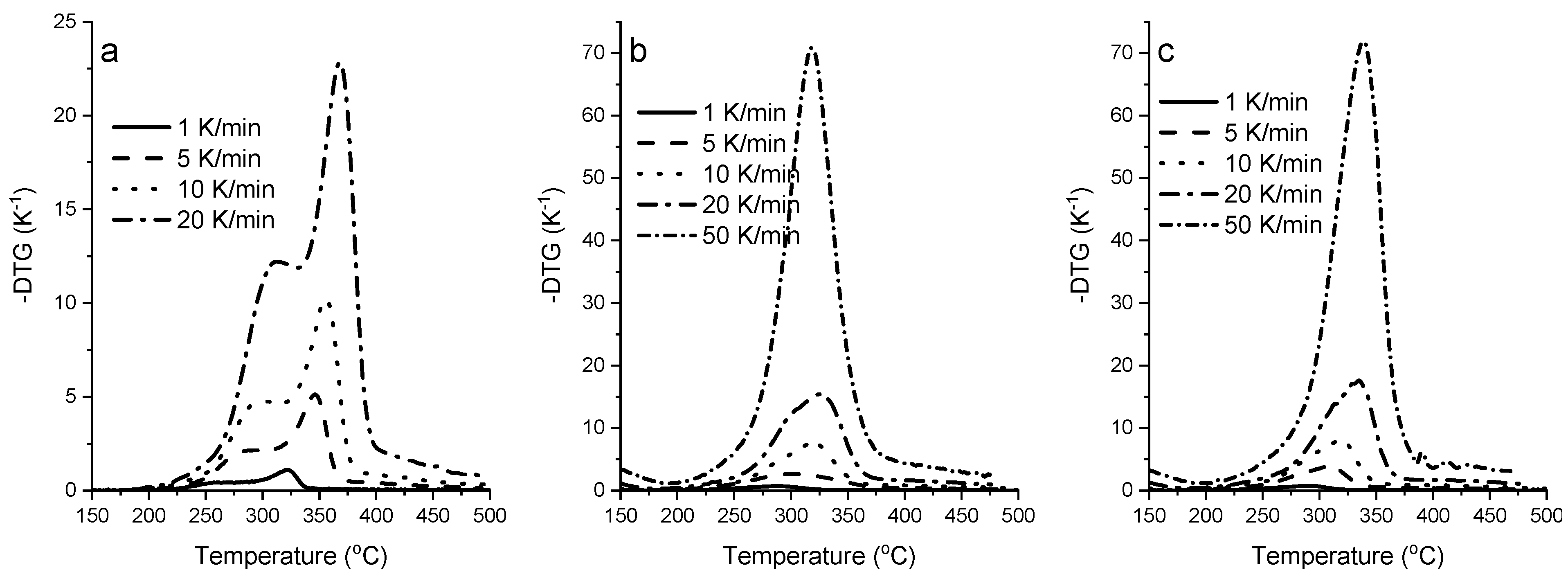
In Figure 2, the DTG profile for each feedstock is shown with higher peaks corresponding to higher heating rates. Additionally, a slight deviation towards higher temperatures (to the right) is observable in the peaks of the curves as the heating rate increases. Numeric data associated with the thermograms are reported in the SI. Char yields (at 900 °C) for beech wood averaged at approximately 25 wt.%, and for the wheat straw, at approximately 27 wt.%, with little variance between the feedstock particle sizes. These values may be attributed to the relatively large sample size for each TGA experiment, as proposed by Anca-Couce et al. [4]. Kornmayer [53] reported comparable values for 1 mm wheat straw (28.5% ± 0.6%) using the same equipment, but no information is given regarding TGA data and its treatment.
In a DTG curve, the cellulose peak is, by convention, the tallest peak; however, for degradation curves such as those of wheat straw, it is often difficult to precisely define where the hemicellulose would be, leading to authors such as Šimkovic and Csomorová [10] characterizing the phenomenon as a single curve encompassing a ‘holocellulosic’ degradation. In several biomasses, including those of beech wood ([4]) or almond shells ([27]), the hemicellulose degradation is identifiable as a ‘shoulder’ or an independent peak at lower temperatures, therefore not requiring this type of treatment.

3.1. Estimation of the Lignocellulosic Composition

Rego et al. [48] employed the deconvolution method of lignocellulosic determination (three pseudo-components) to different poplar wood genotypes and compared it to conventional chemometric measurements; the authors observed a higher coefficient of variation for hemicellulose, between all three, for both the replica measurements (simple genotype) and the chemometric ones. Şen et al. [49] employed both model-fitting (first-order, contracting-sphere, and three-halves models) and deconvolution as separate methods to estimate the lignocellulosic composition of Turkey oak (Quercus cerris) cork, while comparing to chemometric values, and the authors found that first-order model-fitting led to better estimations of cellulose, hemicellulose, and suberin (the sum of both aliphatic and aromatic), but poor estimations of lignin, most likely due to methodological issues. A study by Zhou et al. [54] employed TGA to successfully determine lignocellulosic composition for five different types of biomass with results in the same range as those obtained with conventional methods.
The validity of deconvolution-based methods for lignocellulosic biomass is contested. Maschio et al. [55] indicated the lack of accuracy of thermal decomposition methods, due to the complexity of this kind of structure. The same publication refers to the potential of this method after the hemicellulose content is removed through hydrolysis. Caballero et al. [56] referred to the heterogeneity of the lignocellulosic materials as a deterrent: even between samples of the same crop, the features of the individual organism, such as age and growth factors, lead to large ranges of possible results, especially due to uncertainty in estimating the amount of lignin.
The results presented in Table 5 reflect the pair temperature/conversion for each degradation step considered when using the method proposed by Wu et al. [7], using the second-derivative method by Gaitán-Álvarez et al. [11], and exemplified in Figure 1. The beech wood employed was supplied in the context of another publication [4]. The authors reported, using the same equipment, shoulder temperatures (hemicellulose in Table 5, Beech) of 267.6 °C, 293.5 °C, 309.8 °C, and 321.0 °C for 1, 5, 10, and 20 K·min−1, respectively, as well as peak temperatures of 321.5 °C, 344.2 °C, 355.3 °C, and 367.5 °C, respectively, for the same heating rates. While the peak temperatures reported for cellulose were essentially equal, those for hemicellulose are often higher than those reported in this work. Regarding the conversions, the values selected are 0.261 for the shoulder and 0.693 for the peak, again essentially equal in the case of cellulose and slightly divergent in the case of hemicellulose. The authors selected a conversion for lignin of 0.92, which is higher than the values reported in this work for low heating rates.
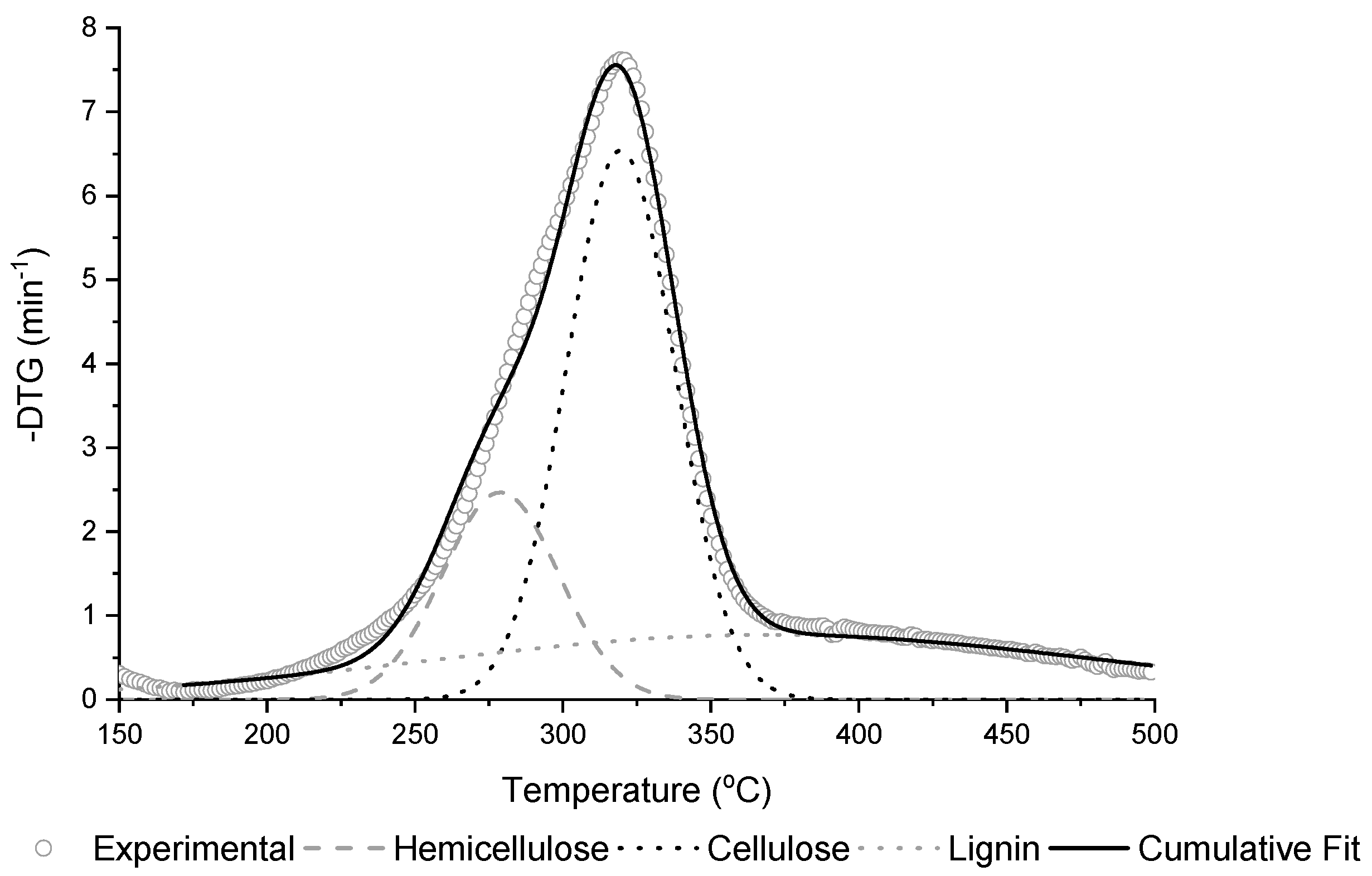
In Table 6, a comparison between the estimated values for each lignocellulosic pseudo-component using the different methods is presented (simple deconvolution and as a variable during model-fitting). These results show that the deconvolution method performs worse than model-fitting methods where the kinetic parameters are also estimated simultaneously. As can be seen in Figure 3, there is considerable overlap between the three pseudo-components due to concurrent degradation, which impacts the feasibility of Gaussian deconvolution methods for biomasses such as wheat straw. When comparing the two different particle sizes (WS-P and WS-H), no consistent difference was found when using these two methods.
The values in Table 7 show the average error of estimation using the different methods in comparison to the reference, taken to be the literature values in Table 6. The lowest error was found for cellulose, which is determined by the highest peak. As the different components of the lignocellulosic matrix undergo simultaneous degradation, the authors suggest that the error stems from the fitting curve overlapping, which may lead to some areas of each peak being assigned to another peak for the same temperature.
The errors for lignin are the highest, with the error of deconvolution being even higher, which may indicate the shortcomings of the methodology. To obtain the deconvolution results, the temperature of the center of each Gaussian peak was set to the value presented in Table 6. Defining the peak point for the lignin curve on the slope change may have led to a large contribution of the charring reaction at high temperatures.

3.2. Comparison of Estimated Kinetic Results

The determination of the shape of a degradation curve using thermogravimetry with Arrhenius parameters can be elusive due to the often unpredictable effects of small changes in the values of these parameters. In that sense, while several publications have discussed the numeric values of the kinetic parameters obtained using isoconversional methods, seldom are such values employed/compared with the DTG curves in a graphic manner. In this section, the curves obtained using the isoconversional methods, and the curve-fitting methods are overlapped with the DTG curve for the sake of comparison.
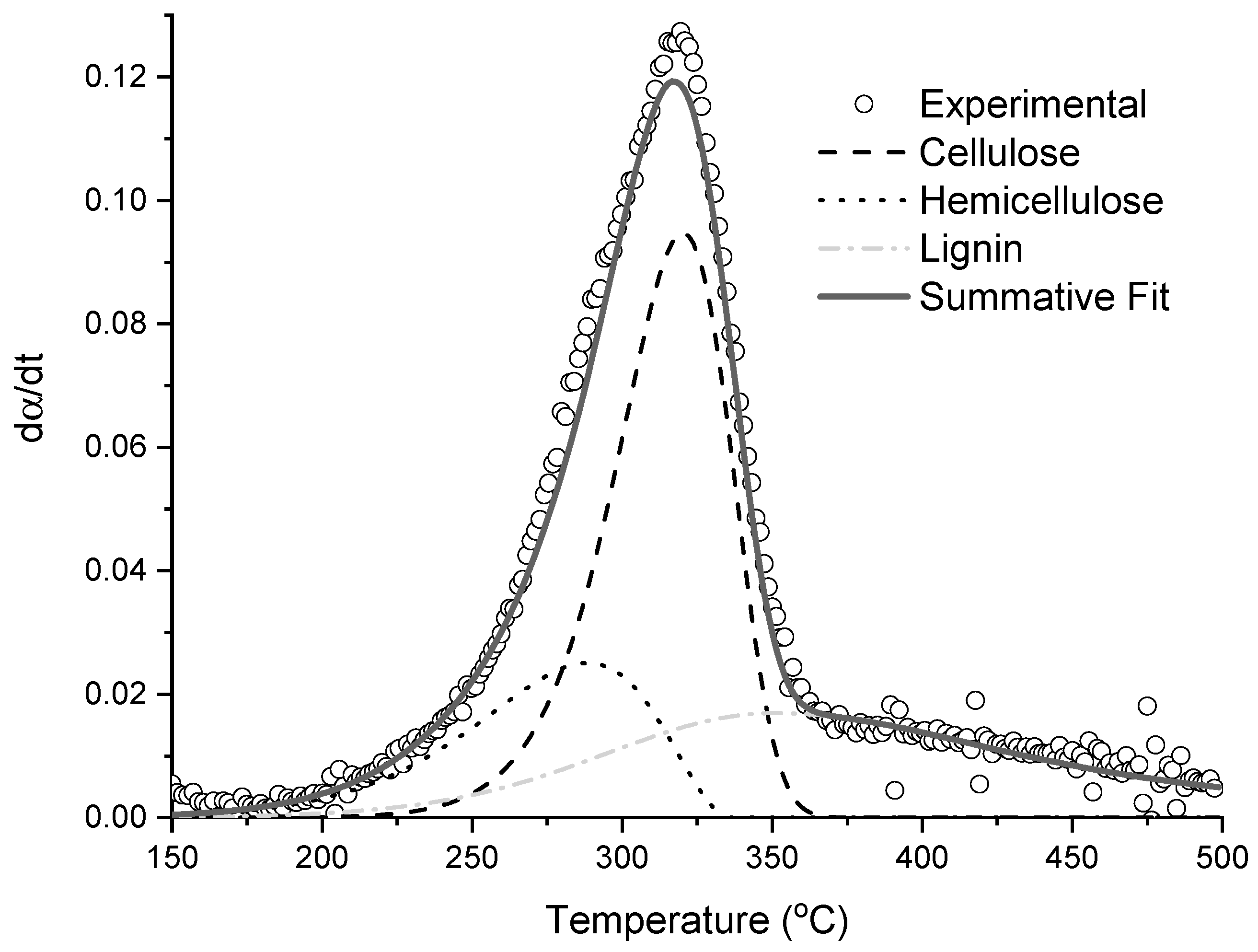
The values of the curve-fitting methods were obtained by fitting all experimental curves of a feedstock simultaneously. On the other hand, to estimate the isoconversional method-derived Arrhenius parameters for each compound (cellulose, hemicellulose, and lignin) of a feedstock, a weighted average was made of the estimated conversion values representative of each compound based on the average of the results of the deconvolution. All numeric values can be found in the SI, as well as the graphical demonstration of the model-fitting procedures. An example of the application of a curve-fitting method is shown in Figure 4, where the reader can see the level of overlap between the different curves at the same temperature, which affects the values of the accrued kinetic parameters.
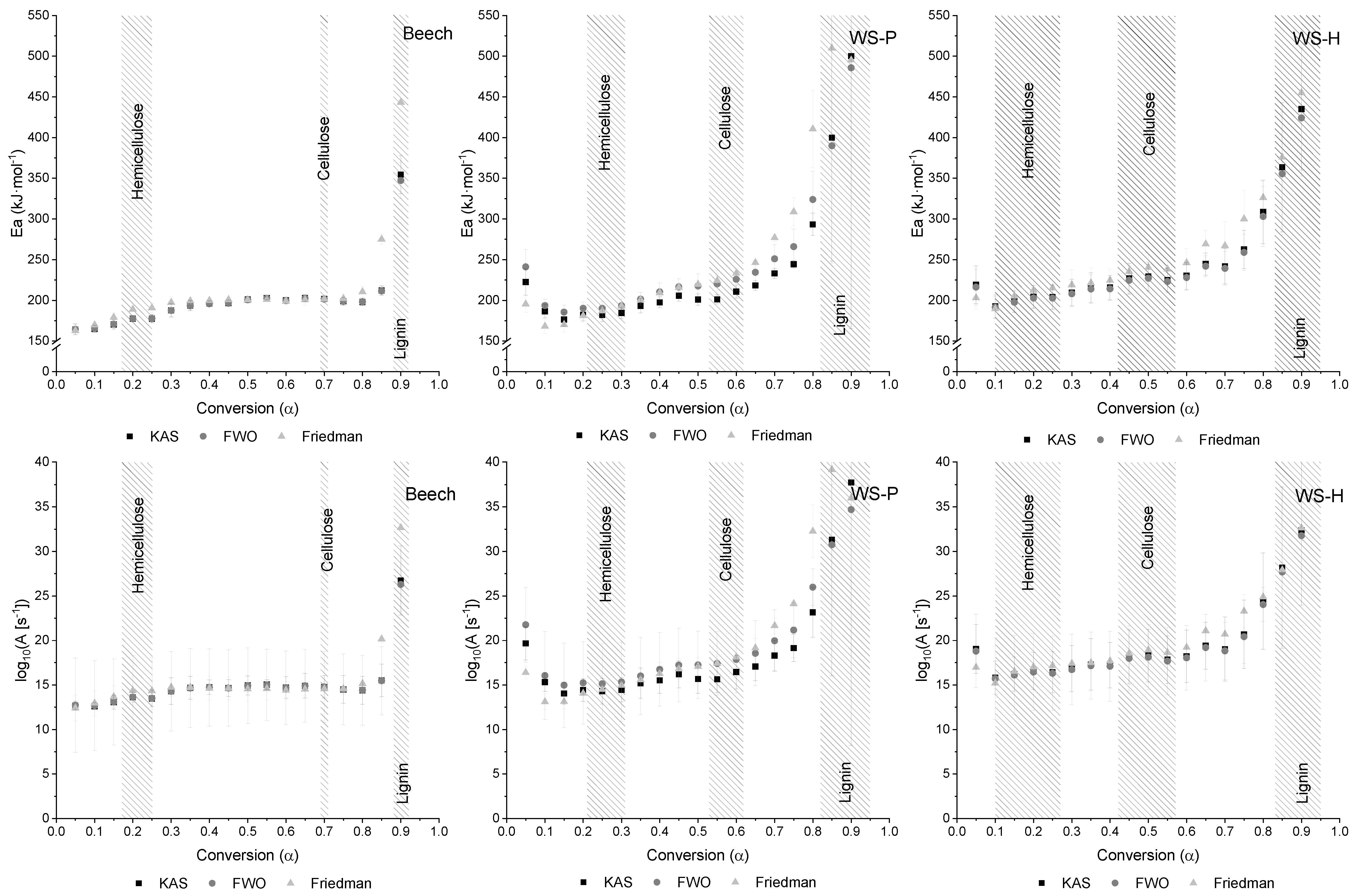
The values for the isoconversional methods are displayed as graphs in Figure 5 (numeric values can be found in the SI), where one can see a visual range of conversion values for which apparent reaction energies for each lignocellulosic pseudo-component were taken for further comparison. The ranges of said pseudo-components are based on the ranges of values obtained using the second derivative method (Table 5). The range of values shown in Figure 5 does not include higher conversions due to the unfeasible results which are expected from these methods; therefore, the value for lignin was taken as the last valid one for each case.
It is a common assumption that the isoconversional methods lead to similar results that resemble each other, as can be seen for the KAS and FWO methods, both integral methods based on similar premises. The use of the Friedman method, a differential method, may lead to erroneous estimates, due to the fact that they require an assumption concerning the form of the kinetic equation, whereas the KAS and FWO methods do not [57].
The kinetic parameters obtained using all methods were collected in Table 8 (cellulose), Table 9 (hemicellulose), and Table 10 (lignin), to ease the comparison. Table 11 shows the root mean square error (RMSE) between the experimental results and curves traced using the kinetic parameters obtained, in which a lower value indicates a better fit.
As seen in Table 11, Isoconversional kinetic parameters derived from the powder samples (Beech and WS-P) are more similar to each other than with the hull sample (WS-H) for hemicellulose and lignin due to the differences in particle size, and may be associated with the heat/mass-transfer limitations because of unconventionally high sample sizes, or even due to the method of identification of the peak conversion value. The values obtained from the hull (not-milled) wheat straw were slightly higher for cellulose and hemicellulose, but lower for lignin.
The curve-fitting method leads to lower errors (Table 11) than the isoconversional methods, as they are directly determined from the experimental data while producing substantially different kinetic parameters, with a difference range to the equivalent isoconversional parameters of 1.7–57.3 kJ·mol−1/1.2–105 s−1 for cellulose, 4.6–78.5 kJ·mol−1/12–107 s−1 for hemicellulose, and 100.0–456.1 kJ·mol−1/102–1036 s−1 for lignin. Despite these differences, the obtained curves show small deviations in shape and peak temperature, and it must be kept in mind that the phenomena of curve overlap are actively occurring, indicating the presence of concurrent reactions, and thus lowering the obtained activation energy of any individual phenomenon.
The kinetic parameters obtained using the KAS and FWO methods are very similar, with an exception in wheat straw powder cellulose, leading to very similar average deviations (Table 11). The similar Friedman method, based on different premises, leads to activation energies similar to the other isoconversional methods, but higher pre-exponential factors for the case of lignin. When comparing the effect of setting the reaction order to 3 instead of 1 for lignin, following the proposal by Manyà et al. [17], when employing the kinetics derived from isoconversional methods for each compound, the differences in the peak position and deviation from the experimental data lead to a consistent ~3% improvement in the fit.
In contrast to the data presented in the introduction, namely the value obtained by Lopéz et al. [36], as shown in Table 1, in which the authors presented values within the range of those obtained in the context of this work, albeit with lower values for both (hemicellulose and lignin) ends of the range, a fact that may have to do with the lower heating rates used in that work in comparison to this one, or with the employed conversion range. Regarding the curve-fitting values, these can be more directly related to the lignin values obtained in the context of this work, both because of the lower heating rates and also due to considering a more extensive temperature range, thus perhaps factoring in charring effects.
The best overall accuracy for all three feedstocks was obtained using the free-order model, due to it having fewer model constraints. Possibly attributed to the aforementioned heat/mass transfer limitations, WS-W presents consistently worse fits than WS-P (except when using the Friedman method). The clear ‘shoulder’ attributed to hemicellulose favors the estimation of this pseudo-component for the beech wood curve-fitting methods, whilst the WS methods present more overlap.
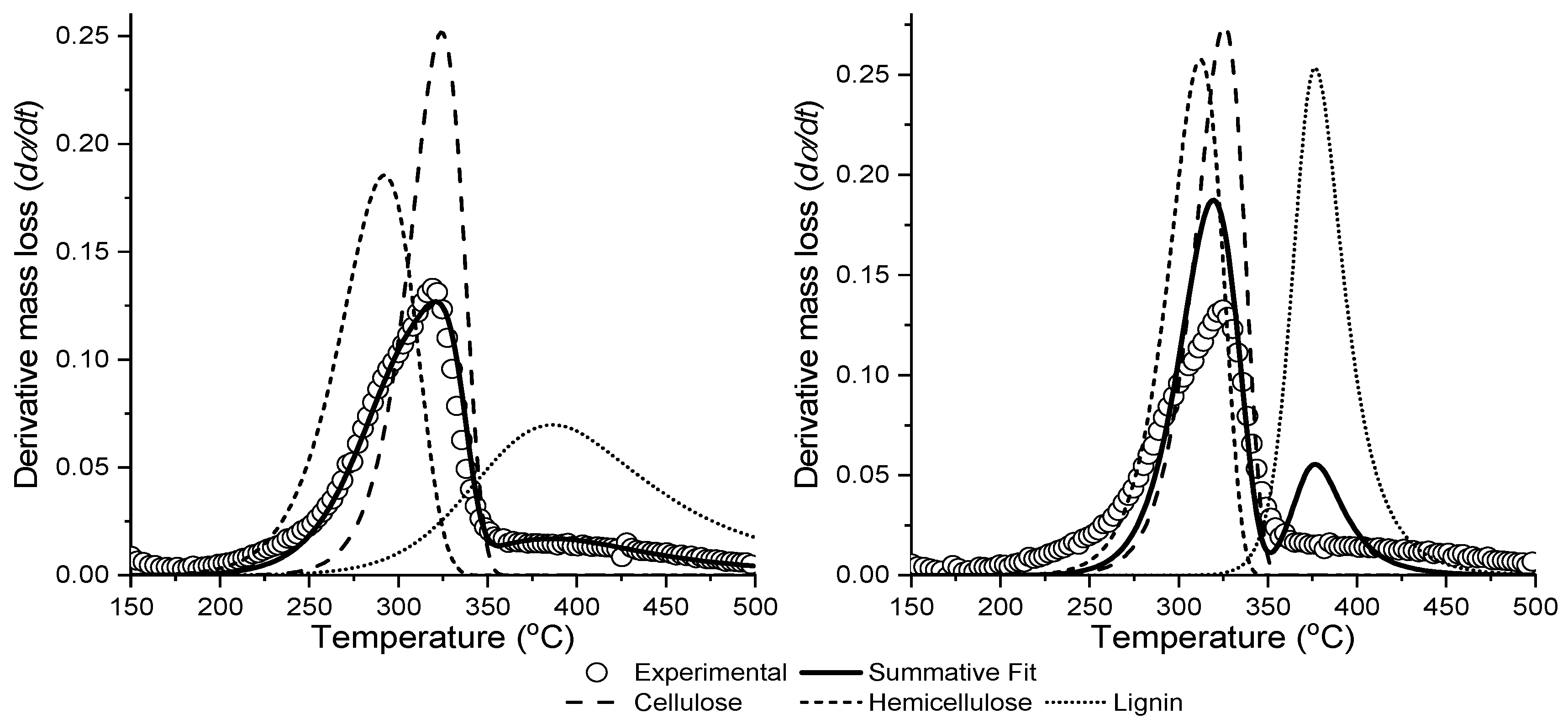
The difference in errors is not enough to completely discard the isoconversional (KAS, FWO, and Friedman) methods on their own since both methods can be regarded as complementary. This manuscript shows that applying isoconversional methods to the kinetic determination of each compound in lignocellulosic biomass is a viable alternative to low application demand. However, this method tends to predict a delay in hemicellulose degradation, which is probably caused by the overlap of cellulose and hemicellulose at the conversions where hemicellulose peaks. This phenomenon is shown in Figure 6.

3.3. Performance of Published Reaction Networks

The degradation of the solid pseudo-components based on the published reaction networks [12,13,14,20,21,22,23,26] was plotted against that of beech wood (powder) and wheat straw (powder (WS-P) and hull (WS-H)) to compare the performance of these networks in simulating the degradation of the biomasses.
All models employ two PCs to model the degradation of cellulose (cellulose and activated cellulose), and three PCs to model hemicellulose (hemicellulose, hemicellulose 1 and 2 (HCE1 and 2)). Of all models reported here, Ranzi et al. [21,22] and Debiagi [23] considered the effects of different hemicellulose (HCE) compositions: the former contrasting the degradation of arabinoxylan-rich materials (softwoods, HCE1/HCE2 = 70/30) with that of galactomannan-rich ones (hardwoods, HCE1/HCE2 = 35/65), and the latter adding grass and cereal feedstocks (HCE1/HCE2 = 12/88) [23]. Based on hemicellulose composition, both beech wood and wheat straw are considered arabinoxylan-rich [45,58].
Regarding lignin, the most common approach is that of three primary PCs (lignins C, H, and O), which degrade into three secondary PCs (lignin-CC, -OH, and “Lig”), as introduced by Ranzi et al. [12]. However, Faravelli et al. [14] developed a radical-based model featuring seven initial lignin representatives and a complex set of intermediaries, but did not lead to a particular improvement in terms of the modeling results.
Table 12 shows the deviations between the summative fit curves and the experimental results for the three feedstocks. Evaluation is primarily based on the derivative deviation, and every model predicts the degradation of beech wood consistently better than it predicts any of the wheat straw particle sizes, except for the case of the Ranzi–Faravelli [12,14,59] network, and the difference between powder and hull wheat straw is lower than 2.5% for all networks. This fact is not surprising, as the detailed degradation schemes commonly use low-ash feedstocks such as wood as reference biomasses during development.
The RAC model [13,24] is the best performing for beech wood, followed by the Corbetta [20], the Ranzi (17a) [21], and the Ranzi (08) [12] models. For the cases of both wheat straw feedstocks, the lowest deviations were found for the Corbetta [20], while the second place was taken by the Ranzi (08) [12] model, followed by the RAC [13,24] and Ranzi (17a) [21] models. A visual representation of the best results (derivatives) can be found in Figure 7, and a representation of the individual component curves can be found in the SI.

Influence of Potassium Content on the Pyrolysis of Cellulose

Trendewicz et al. [26] proposed alternative kinetic parameters for the degradation of active cellulose and the charring of crystal cellulose depending on the potassium content of the feedstock. For the best four cases in Table 12, the original cellulose degradation networks were partially replaced with the Trendewicz model, of which the deviations from the experimental results are shown in Table 13.
The fact that the presence of ash leads to higher deviations for beech than for straw—deviations which are often higher than curves not considering this factor—may stem from overlap with the hemicellulose curve due to the shift to lower temperatures, leading to a less pronounced hemicellulose shoulder, and thus higher deviations. This phenomenon does not occur for wheat straw due to the absence of a pronounced shoulder.
The results found in Table 13 indicate that taking into consideration the potassium influence often leads to better fits (lower deviations) for wheat straw, mostly because of a peak shift to lower temperatures (catalyzed reaction, as shown in Figure 7). However, the experimental value of the potassium content of wheat straw (1.18 wt.%) is outside the range of values employed by Trendewicz et al. [26] to calibrate the model, thus presenting very high deviations in all cases.
The best values (‘Best B’ and ‘Best WS’) were estimated to find the potassium content for which the fit of each reaction network presents the lowest deviation for beech and WS-P/WS-H, respectively, estimated using GRG nonlinear solver (bundled with Microsoft Excel™ 2016). Apart from the Ranzi (17a) model [21], the optimum potassium content for beech is very close to null. For the case of wheat straw, the optimum is found for values much lower than the experimentally determined value, indicating the need to calibrate this model by taking into consideration the real biomass, and not just isolated cellulose.
That said, the best models to model the degradation of beech wood are the unmodified networks presented in Table 13. For the case of straw, deviations are marginally different between powder and hull. Based exclusively on the derivative error, the best results are found for the RAC [13,24], followed by the Corbetta model [20], the Ranzi (17a) model [21], and the Ranzi (08) model [12], all of which employ a potassium content named Best WS. A visual representation of the influence of the changing cellulose peak height and position can be found in Figure 8.

4. Conclusions

This paper presents the experimental determination of kinetic parameters for the pyrolysis of wheat straw as a representative of high ash content biomass. Two fundamental challenges were addressed to obtain these parameters which are due to the catalytic effects of (earth) alkali metals that often occur in biomass with a high ash content.
First, wheat straw degradation is characterized by a single decomposition stage (a single peak in the derivative curve (DTG)) due to its high ash content, which hampers the identification of the degradation of hemicellulose. This problem was solved by applying the second derivative (DDTG) to identify inflection points that can be taken as the peak position of the degradation of the different pseudo-components. To the best of our knowledge, this method does not seem to have been previously implemented for either of the feedstocks employed in the context of this work for the estimation of lignocellulosic composition, presenting an average error of 30 wt. %, when compared to literature values based on conventional chemometric methods. Based on the method results, it is possible to identify conversion values corresponding to the maximum degradation of hemicellulose, cellulose, and lignin, allowing the user to obtain kinetic parameters for these three phenomena based on isoconversional methods (KAS, FWO, and Friedman), or as anchor points for curve-fitting by square error minimization assuming the concurrent degradation of lignocellulosic pseudo-components (different orders of reaction considered).
Curve-fitting methods predictably lead to better fits when testing the obtained kinetic parameters, while the values derived from the use of isoconversional methods to determine the kinetics of each compound often present a delay in the hemicellulose degradation. However, a higher error should not be indicative of the unfeasibility of this method, as despite this fact, it has a much higher simplicity of application. The comparison between the powder and hull particle sizes showed a small but significant deviation, probably due to the thin walls of wheat straw hulls.
Secondly, it was confirmed that reaction networks available in the literature–which have been primarily developed for biomass with a low ash content—can also be used to describe the degradation of biomass with a high ash content. Kinetic parameters from seven published reaction networks designed to model the pyrolysis of biomass were employed to model degradation curves which were contrasted with experimental data to evaluate their feasibility for modeling the degradation of the feedstocks being studied in this work. Among the reaction networks tested, the best results (lowest derivative deviation) were found for the Ranzi (08) [12], Corbetta [20], RAC [13,24], and Ranzi (17a) [21] models. As expected, deviations between the experimental behavior and model results using reaction networks were found to be lower for beech wood compared to wheat straw.
It is a known fact that potassium catalyzes the degradation of cellulose, shifting the derivative curve (DTG) to lower temperatures and higher peaks. Trendewicz et al. [26] developed an alternative model for the degradation of cellulose, which considers the effect of the feedstock potassium content and was implemented in the seven aforementioned reaction networks. While a potassium content of 0.10 wt.% (beech wood) leads to a minor shift, it was ultimately found that it does not lead to a better fit to beech experimental data. A potassium content of 1.18 wt.% (wheat straw) leads to both excessively tall peaks at low temperatures, leading to worse fits than the original reaction networks. Based on the alternative model, we were able to estimate the potassium contents for which the experimental data are best modeled, allowing for more accurate modeling.
Future work indubitably lies in the application of the obtained kinetic parameters to model the degradation of wheat straw using fast pyrolysis, as the considerable differences in heating rate may lead to non-optimal results. In addition, improving on the current model of Trendewicz et al. [26] by considering not only a larger range of ash contents but also complete biomass—rather than only isolated cellulose—may lead to more exact results. Other options for future work may lie in the comparison of more recently developed methods for the estimation of degradation kinetics. The application of a simple Newton method for the numerical estimation of the second derivative incurs an error proportional to the square of the step size, and more novel methods with lower errors may be employed.
Kinetic parameters for wheat straw are scarcely available in the literature. They show a wide range of values which are not associated with individual lignocellulosic pseudo-components, but rather assume a single-stage decomposition of the material. By applying the presented methodology, this problem could be solved and a more reliable description of wheat straw pyrolysis, as representative for biomass with high ash content, was derived.

Supplementary Materials

The following supporting information can be downloaded at: https://www.mdpi.com/article/10.3390/en15197240/s1.

Author Contributions

Conceptualization, F.G.F.; Data curation, A.A.-C.; Funding acquisition, N.D.; Methodology, A.A.-C.; Project administration, N.D.; Supervision, A.F.; Writing—original draft, F.G.F.; Writing—review and editing, A.A.-C. and A.F. All authors have read and agreed to the published version of the manuscript.

Funding

This work has received funding from the European Union’s Horizon 2020’s research and innovation programme under grant agreement number 731101.

Acknowledgments

The authors acknowledge support from the KIT-Publication Fund of the Karlsruhe Institute of Technology. The authors acknowledged the assistance of Umut Ali Şen with the setup of the kinetic schemes, as well as the staff at the Brennstoff Labor at IKFT-KIT and Iuliia Tishina for the TGA analyses. One of the authors (F.G. Fonseca) is a member of the Bioeconomy Graduate Program BBW ForWerts.

Conflicts of Interest

The authors declare no conflict of interest. The funders had no role in the design of the study; in the collection, analyses, or interpretation of data; in the writing of the manuscript; or in the decision to publish the results.

References

  1. Anca-Couce, A.; Berger, A.; Zobel, N. How to determine consistent biomass pyrolysis kinetics in a parallel reaction scheme. Fuel 2014, 123, 230–240. [Google Scholar] [CrossRef]
  2. Humbird, D.; Trendewicz, A.; Braun, R.; Dutta, A. One-Dimensional Biomass Fast Pyrolysis Model with Reaction Kinetics Integrated in an Aspen Plus Biorefinery Process Model. ACS Sustain. Chem. Eng. 2017, 5, 2463–2470. [Google Scholar] [CrossRef]
  3. White, J.E.; Catallo, W.J.; Legendre, B.L. Biomass pyrolysis kinetics: A comparative critical review with relevant agricultural residue case studies. J. Anal. Appl. Pyrolysis 2011, 91, 1–33. [Google Scholar] [CrossRef]
  4. Anca-Couce, A.; Tsekos, C.; Retschitzegger, S.; Zimbardi, F.; Funke, A.; Banks, S.; Kraia, T.; Marques, P.; Scharler, R.; de Jong, W.; et al. Biomass pyrolysis TGA assessment with an international round robin. Fuel 2020, 276, 118002. [Google Scholar] [CrossRef]
  5. Cai, J.; Xu, D.; Dong, Z.; Yu, X.; Yang, Y.; Banks, S.W.; Bridgwater, A.V. Processing thermogravimetric analysis data for isoconversional kinetic analysis of lignocellulosic biomass pyrolysis: Case study of corn stalk. Renew. Sustain. Energy Rev. 2018, 82, 2705–2715. [Google Scholar] [CrossRef] [Green Version]
  6. Espenson, J. Chemical Kinetics and Reaction Mechanisms, 2nd ed.; McGraw-Hill: New York, NY, USA, 1995; ISBN 9780070202603. [Google Scholar]
  7. Wu, W.; Mei, Y.; Zhang, L.; Liu, R.; Cai, J. Kinetics and reaction chemistry of pyrolysis and combustion of tobacco waste. Fuel 2015, 156, 71–80. [Google Scholar] [CrossRef]
  8. Sher, F.; Iqbal, S.Z.; Liu, H.; Imran, M.; Snape, C.E. Thermal and kinetic analysis of diverse biomass fuels under different reaction environment: A way forward to renewable energy sources. Energy Convers. Manag. 2020, 203, 112266. [Google Scholar] [CrossRef]
  9. Manić, N.; Jankovic, B.; Stojiljkovic, D.; Jovanovic, V.; Radojevic, M. TGA-DSC-MS analysis of pyrolysis process of various agricultural residues. Therm. Sci. 2019, 23, 1457–1472. [Google Scholar] [CrossRef] [Green Version]
  10. Šimkovic, I.; Csomorová, K. Thermogravimetric analysis of agricultural residues: Oxygen effect and environmental impact. J. Appl. Polym. Sci. 2006, 100, 1318–1322. [Google Scholar] [CrossRef]
  11. Gaitán-Álvarez, J.; Moya, R.; Puente-Urbina, A.; Rodriguez-Zúñiga, A. Thermogravimetric, devolatilization rate, and differential scanning calorimetry analyses of biomass of tropical plantation species of Costa Rica torrefied at different temperatures and times. Energies 2018, 11, 696. [Google Scholar] [CrossRef]
  12. Ranzi, E.; Cuoci, A.; Faravelli, T.; Frassoldati, A.; Migliavacca, G.; Pierucci, S.; Sommariva, S. Chemical Kinetics of Biomass Pyrolysis. Energ. Fuel 2008, 22, 4292–4300. [Google Scholar] [CrossRef]
  13. Anca-Couce, A.; Scharler, R. Modelling heat of reaction in biomass pyrolysis with detailed reaction schemes. Fuel 2017, 206, 572–579. [Google Scholar] [CrossRef]
  14. Faravelli, T.; Frassoldati, A.; Migliavacca, G.; Ranzi, E. Detailed kinetic modeling of the thermal degradation of lignins. Biomass Bioenergy 2010, 34, 290–301. [Google Scholar] [CrossRef]
  15. Di Blasi, C. Modeling chemical and physical processes of wood and biomass pyrolysis. Prog. Energy Combust. Sci. 2008, 34, 47–90. [Google Scholar] [CrossRef]
  16. Yang, H.; Yan, R.; Chen, H.; Lee, D.H.; Zheng, C. Characteristics of hemicellulose, cellulose and lignin pyrolysis. Fuel 2007, 86, 1781–1788. [Google Scholar] [CrossRef]
  17. Manyà, J.J.; Velo, E.; Puigjaner, L. Kinetics of biomass pyrolysis: A reformulated three-parallel-reactions model. Ind. Eng. Chem. Res. 2003, 42, 434–441. [Google Scholar] [CrossRef]
  18. Gomez Diaz, C.J. Understanding Biomass Pyrolysis Kinetics: Improved Modeling Based on Comprehensive Thermokinetic Analysis; Universitat Politècnica de Catalunya: Barcelona, Spain, 2006. [Google Scholar]
  19. Gómez, C.J.; Várhegyi, G.; Puigjaner, L. Slow pyrolysis of woody residues and an herbaceous biomass crop: A kinetic study. Ind. Eng. Chem. Res. 2005, 44, 6650–6660. [Google Scholar] [CrossRef]
  20. Corbetta, M.; Pierucci, S.; Ranzi, E.; Bennadji, H.; Fisher, E.M. Multistep Kinetic Model of Biomass Pyrolysis. In Proceedings of the XXXVI Meeting of the Italian Section of the Combustion Institute, Procida, Italy, 13–15 June 2013; pp. 4–9. [Google Scholar]
  21. Ranzi, E.; Debiagi, P.E.A.; Frassoldati, A. Mathematical Modeling of Fast Biomass Pyrolysis and Bio-Oil Formation. Note I: Kinetic Mechanism of Biomass Pyrolysis. ACS Sustain. Chem. Eng. 2017, 5, 2867–2881. [Google Scholar] [CrossRef] [Green Version]
  22. Ranzi, E.; Debiagi, P.E.A.; Frassoldati, A. Mathematical Modeling of Fast Biomass Pyrolysis and Bio-Oil Formation. Note II: Secondary Gas-Phase Reactions and Bio-Oil Formation. ACS Sustain. Chem. Eng. 2017, 5, 2882–2896. [Google Scholar] [CrossRef]
  23. Debiagi, P.; Gentile, G.; Cuoci, A.; Frassoldati, A.; Ranzi, E.; Faravelli, T. A predictive model of biochar formation and characterization. J. Anal. Appl. Pyrolysis 2018, 134, 326–335. [Google Scholar] [CrossRef]
  24. Pecha, M.B.; Arbelaez, J.I.M.; Garcia-Perez, M.; Chejne, F.; Ciesielski, P.N. Progress in understanding the four dominant intra-particle phenomena of lignocellulose pyrolysis: Chemical reactions, heat transfer, mass transfer, and phase change. Green Chem. 2019, 21, 2868–2898. [Google Scholar] [CrossRef] [Green Version]
  25. Fonseca, F.G.; Funke, A.; Niebel, A.; Soares Dias, A.P.; Dahmen, N. Moisture content as a design and operational parameter for fast pyrolysis. J. Anal. Appl. Pyrolysis 2019, 139, 73–86. [Google Scholar] [CrossRef]
  26. Trendewicz, A.; Evans, R.; Dutta, A.; Sykes, R.; Carpenter, D.; Braun, R. Evaluating the effect of potassium on cellulose pyrolysis reaction kinetics. Biomass Bioenergy 2015, 74, 15–25. [Google Scholar] [CrossRef] [Green Version]
  27. Marcilla, A.; García, A.N.; Pastor, M.V.; León, M.; Sánchez, A.J.; Gómez, D.M. Thermal decomposition of the different particles size fractions of almond shells and olive stones. Thermal behaviour changes due to the milling processes. Thermochim. Acta 2013, 564, 24–33. [Google Scholar] [CrossRef]
  28. Scott, D.S.; Piskorz, J. The flash pyrolysis of aspen-poplar wood. Can. J. Chem. Eng. 1982, 60, 666–674. [Google Scholar] [CrossRef]
  29. Bridgwater, A.V.V. Review of fast pyrolysis of biomass and product upgrading. Biomass Bioenergy 2012, 38, 68–94. [Google Scholar] [CrossRef]
  30. Wang, X.; Kersten, S.R.A.; Prins, W.; Van Swaaij, W.P.M. Biomass pyrolysis in a fluidized bed reactor. Part 2: Experimental validation of model results. Ind. Eng. Chem. Res. 2005, 44, 8786–8795. [Google Scholar] [CrossRef]
  31. Shen, J.; Wang, X.-S.; Garcia-Perez, M.; Mourant, D.; Rhodes, M.J.; Li, C.-Z. Effects of particle size on the fast pyrolysis of oil mallee woody biomass. Fuel 2009, 88, 1810–1817. [Google Scholar] [CrossRef]
  32. Salehi, E.; Abedi, J.; Harding, T. Bio-oil from Sawdust: Effect of Operating Parameters on the Yield and Quality of Pyrolysis Products. Energy Fuels 2011, 25, 4145–4154. [Google Scholar] [CrossRef]
  33. Demirbas, A. Effects of temperature and particle size on bio-char yield from pyrolysis of agricultural residues. J. Anal. Appl. Pyrolysis 2004, 72, 243–248. [Google Scholar] [CrossRef]
  34. Luangkiattikhun, P.; Tangsathitkulchai, C.; Tangsathitkulchai, M. Non-isothermal thermogravimetric analysis of oil-palm solid wastes. Bioresour. Technol. 2008, 99, 986–997. [Google Scholar] [CrossRef] [PubMed]
  35. Pütün, A.E.; Koçkar, Ö.M.; Yorgun, S.; Gerçel, H.F.; Andresen, J.; Snape, C.E.; Pütün, E. Fixed-bed pyrolysis and hydropyrolysis of sunflower bagasse: Product yields and compositions. Fuel Process. Technol. 1996, 46, 49–62. [Google Scholar] [CrossRef]
  36. López Ordovás, J. Construction of a Model for the Design of a Rotary Kiln For Slow Pyrolysis of Biomass—Greencarbon Project; Aston University: Birmingham, UK, 2020. [Google Scholar]
  37. Cai, J.M.; Bi, L.S. Kinetic analysis of wheat straw pyrolysis using isoconversional methods. J. Therm. Anal. Calorim. 2009, 98, 325–330. [Google Scholar] [CrossRef]
  38. Yang, Q.; Wu, S. Wheat straw pyrolysis analysis by thermogravimetry and gas chromatography-mass spectrometry. Cellul. Chem. Technol. 2009, 43, 123–131. [Google Scholar] [CrossRef]
  39. Zhaosheng, Y.; Xiaoqian, M.; Ao, L. Kinetic studies on catalytic combustion of rice and wheat straw under air- and oxygen-enriched atmospheres, by using thermogravimetric analysis. Biomass Bioenergy 2008, 32, 1046–1055. [Google Scholar] [CrossRef]
  40. Rong, H.; Yuan, J.; Feng, Y.; Yi, Y.; Chang, Z. A TG-IR study on the co-pyrolysis characteristics of oily sludge and crops. Biomass Convers. Biorefinery 2020. [Google Scholar] [CrossRef]
  41. Naqvi, S.R.; Ali, I.; Nasir, S.; Ali Ammar Taqvi, S.; Atabani, A.E.; Chen, W.-H. Assessment of agro-industrial residues for bioenergy potential by investigating thermo-kinetic behavior in a slow pyrolysis process. Fuel 2020, 278, 118259. [Google Scholar] [CrossRef]
  42. Luo, L.; Guo, X.; Zhang, Z.; Chai, M.; Rahman, M.M.; Zhang, X.; Cai, J. Insight into Pyrolysis Kinetics of Lignocellulosic Biomass: Isoconversional Kinetic Analysis by the Modified Friedman Method. Energy Fuels 2020, 34, 4874–4881. [Google Scholar] [CrossRef]
  43. Wu, J.; Liao, Y.; Lin, Y.; Tian, Y.; Ma, X. Study on thermal decomposition kinetics model of sewage sludge and wheat based on multi distributed activation energy. Energy 2019, 185, 795–803. [Google Scholar] [CrossRef]
  44. Mureddu, M.; Dessì, F.; Orsini, A.; Ferrara, F.; Pettinau, A. Air- and oxygen-blown characterization of coal and biomass by thermogravimetric analysis. Fuel 2018, 212, 626–637. [Google Scholar] [CrossRef]
  45. Peng, Y.; Wu, S. The structural and thermal characteristics of wheat straw hemicellulose. J. Anal. Appl. Pyrolysis 2010, 88, 134–139. [Google Scholar] [CrossRef]
  46. Yang, Q.; Wu, S.; Lou, R.; Lv, G. Analysis of wheat straw lignin by thermogravimetry and pyrolysis-gas chromatography/mass spectrometry. J. Anal. Appl. Pyrolysis 2010, 87, 65–69. [Google Scholar] [CrossRef]
  47. Yew, A.C. Numerical Differentiation: Finite Differences; Brown University: Providence, RI, USA, 2011. [Google Scholar]
  48. Rego, F.; Dias, A.P.S.; Casquilho, M.; Rosa, F.C.; Rodrigues, A. Fast determination of lignocellulosic composition of poplar biomass by Thermogravimetry. Biomass Bioenergy 2019, 122, 375–380. [Google Scholar] [CrossRef]
  49. Şen, A.U.; Fonseca, F.G.; Funke, A.; Pereira, H.; Lemos, F. Pyrolysis kinetics and estimation of chemical composition of Quercus cerris cork. Biomass Convers. Biorefinery 2020. [Google Scholar] [CrossRef]
  50. Carrier, M.; Auret, L.; Bridgwater, A.; Knoetze, J.H. Using apparent activation energy as a reactivity criterion for biomass pyrolysis. Energy Fuels 2016, 30, 7834–7841. [Google Scholar] [CrossRef] [Green Version]
  51. Vyazovkin, S.; Burnham, A.K.; Criado, J.M.; Pérez-Maqueda, L.A.; Popescu, C.; Sbirrazzuoli, N. ICTAC Kinetics Committee recommendations for performing kinetic computations on thermal analysis data. Thermochim. Acta 2011, 520, 1–19. [Google Scholar] [CrossRef]
  52. Hindmarsh, A.C.; Petzold, L.R. Algorithms and software for ordinary differential equations and differential- algebraic equations, Part I: Euler methods and error estimation. Comput. Phys. 1995, 9, 34. [Google Scholar] [CrossRef] [Green Version]
  53. Kornmayer, C. Verfahrenstechnik Untersuchungen zur Schnellpyrolyse von Lignocellulose im Doppenschnecken-Mischreaktor; Universität Fridericiana Karlsruhe: Karlsruhe, Germany, 2009. [Google Scholar]
  54. Zhou, H.; Long, Y.; Meng, A.; Li, Q.; Zhang, Y. The pyrolysis simulation of five biomass species by hemi-cellulose, cellulose and lignin based on thermogravimetric curves. Thermochim. Acta 2013, 566, 36–43. [Google Scholar] [CrossRef]
  55. Maschio, G.; Cozzani, V.; Lucchesi, A.; Stoppato, G.; Maschio, G. A New Method to Determine the Composition of Biomass by Thermogravimetric Analysis. Can. J. Chem. Eng. 1997, 75, 127–133. [Google Scholar] [CrossRef]
  56. Caballero, J.A.; Font, R.; Marcilla, A. Comparative study of the pyrolysis of almond shells and their fractions, holocellulose and lignin. Product yields and kinetics. Thermochim. Acta 1996, 276, 57–77. [Google Scholar] [CrossRef]
  57. Venkatesh, M.; Ravi, P.; Tewari, S.P. Isoconversional Kinetic Analysis of Decomposition of Nitroimidazoles: Friedman method vs. Flynn–Wall–Ozawa Method. J. Phys. Chem. A 2013, 117, 10162–10169. [Google Scholar] [CrossRef] [PubMed]
  58. Wang, J.; Minami, E.; Kawamoto, H. Thermal reactivity of hemicellulose and cellulose in cedar and beech wood cell walls. J. Wood Sci. 2020, 66, 41. [Google Scholar] [CrossRef]
  59. Peters, J.F.; Banks, S.W.; Bridgwater, A.V.; Dufour, J. A kinetic reaction model for biomass pyrolysis processes in Aspen Plus. Appl. Energy 2017, 188, 595–603. [Google Scholar] [CrossRef]
Figure 1. Use of the second derivative (DDTG, in black) inflection points to determine the peak/transition points for the different pseudo-components (PCs) based on the works of Gaitán-Álvarez et al. [11] and Wu et al. [7]. Example using wheat straw hull at 10 K·min−1.
Energies 15 07240 g001
Figure 2. Comparison of the DTG behavior divided by feedstock: (a) beech; (b) WS-P; and (c) WS-H.
Energies 15 07240 g002
Figure 3. Example of deconvolution using Gaussian curves centered at the point devised by the DDTG method (see Table 5). WS-P, 10 K·min−1.
Energies 15 07240 g003
Figure 4. Example of curve-fitting using Arrhenius curves. Initial guess for each curve centered at the point devised by the DDTG method (see Table 5). WS-P, 10 K·min−1.
Energies 15 07240 g004
Figure 5. Kinetic parameters obtained using the isoconversional methods. Top: activation energy; bottom: pre-exponential factor. Values for higher conversions were disregarded.
Energies 15 07240 g005
Figure 6. Comparison of the curve-fitting n3 = 3 method (left) and the isoconversional KAS (n3 = 3) method (right). Experimental data: DTG from WS-P, 10 K·min−1.
Energies 15 07240 g006
Figure 7. Comparison of the experimental degradation (above: mass loss; below: derivative) curves with the network curves with the lowest deviations towards WS-H. R08 = Ranzi et al. [12]; C13 = Corbetta [20]; RAC = Anca-Couce and Scharler [13,24]; and R17a = Ranzi et al. [21].
Energies 15 07240 g007
Figure 8. Comparison of the experimental derivative degradation curves with the predictions of the R17a model [21] modified using the Trendewicz model [26] assuming three different potassium contents: (A) cellulose curves against WS-H experimental degradation; (B) summative curves against WS-H experimental degradation; (C) cellulose curves against beech experimental degradation; and (D) summative curves against beech experimental degradation.
Energies 15 07240 g008
Table 1. Arrhenius parameters for the non-catalytic degradation of wheat straw (WS) taken from the work of Lopez et al. [36].
MethodTemperature Range (°C)Heating Rates (K·min−1)Ea (kJ·mol−1)log10 (A (s−1))
KASα 0.10–0.70 a1, 2.5, 5214–35319.1–32.8
FWOα 0.10–0.70 a1, 2.5, 5215–34719.2–32.3
Friedmanα 0.10–0.70 a1, 2.5, 5218–53519.7–48.4
Curve Fitting100–9001, 2.5, 5226.9021.03
a No temperature data were provided, just the variation with the conversion.
Table 2. Literature data of Arrhenius parameters for the non-catalytic degradation of wheat straw (WS).
MethodTemperature
Range (°C)
Heating Rates
(K·min−1)
Ea (kJ·mol−1)log10 (A (s−1))Reference
FWO315–3925, 10, 20130–175-[37]
Kissinger220–40010, 20, 30, 40, 5093.923.03[38]
Coats–Redfern198–33830115.5911.97[39]
Coats–Redfern338–8403024.263.42[39]
Coats–Redfern a220–2601069-[10]
Coats–Redfern251–347208.81-[40]
Coats–Redfern
(First Order Model)
250–400540.845.55[41]
Coats–Redfern
(3D diffusion model)
250–400582.446.99[41]
Coats–Redfern
(Geometric contraction)
250–400536.539.06[41]
Coats–Redfern
(Avarami–Erofe’ev)
250–400515.735.53[41]
Coats–Redfern
(Power Law)
250–40059.705.53[41]
Modified Friedmanα 0.05–0.60b2.5, 5, 10, 20154–176-[42]
Modified Friedmanα 0.60–0.85 b2.5, 5, 10, 20176–379-[42]
DAEM177–52740, 45, 50236–3822.95[43]
Unrecognized c215–3152098.98-[8]
a: Referred to by the authors as the “linear regression method”; b: No temperature data were provided, just the variation with the conversion. c: Referred to by the authors as “based on Arrhenius equation”, based on Mureddu et al. [44].
Table 3. Literature data of Arrhenius parameters for the non-catalytic degradation of wheat straw (WS) fractions.
FeedstockMethodTemperature
Range (°C)
Heating Rates
(K·min−1)
Ea
(kJ·mol−1)
log10
(A (s−1))
Reference
Hemicellulose WSCoats–Redfern160–3505, 10, 20, 3088–977.42–8.90[45]
Hemicellulose WSCoats–Redfern350–5505, 10, 20, 3053–592.80–3.72[45]
Enzymatic Acidolysis
WS Lignin
Kissinger343–39210, 20, 30, 40, 50103.923.06[46]
Enzymatic Acidolysis
WS Lignin
Ozawa343–39210, 20, 30, 40, 50107.693.09[46]
Table 4. Proximate, ultimate, and elemental analysis of the feedstocks used in the work. All values in dry base.
BeechWS-PWS-H
Moisture (wt.%)9.09.39.2
Ash (wt.%)1.06.97.0
Volatile Matter (wt.%)81.767.567.5
Ultimate Analysis
C (wt.%)47.343.843.8
H (wt.%)6.16.16.1
N (wt.%)<0.3<1<1
S (wt.%)0.020.090.09
Ca (ppm)264437803780
K (ppm)95511,80011,800
Si (ppm)652122,60022,600
Table 5. Results of the second-derivative study. Temperature in °C.
Heating Rate (K min−1)Beech
HemicelluloseCelluloseLignin
1T = 260.6 ± 0.5
α = 0.17 ± 0.01
T = 322.9 ± 0.1
α = 0.71 ± 0.00
T = 344.8 ± 0.4
α = 0.88 ± 0.00
5T = 294.3 ± 0.9
α = 0.25 ± 0.00
T = 345.1 ± 0.7
α = 0.69 ± 0.00
T = 370.0 ± 1.1
α = 0.89 ± 0.00
10T = 299.1 ± 0.6
α = 0.22 ± 0.01
T = 354.9 ± 0.2
α = 0.69 ± 0.00
T = 391.3 ± 0.8
α = 0.91 ± 0.00
20T = 312.2
α = 0.23
T = 368.3
α = 0.71
T = 400.3
α = 0.92
Heating Rate (K min−1)WS-P
1T = 263.3 ± 2.5
α = 0.26 ± 0.03
T = 288.6 ± 0.5
α = 0.53 ± 0.00
T = 330.6 ± 5.4
α = 0.82 ± 0.01
5T = 275.5 ± 3.4
α = 0.21 ± 0.01
T = 310.9 ± 1.9
α = 0.57 ± 0.00
T = 353.5 ± 2.4
α = 0.84 ± 0.00
10T = 283.5 ± 1.6
α = 0.21 ± 0.00
T = 321.4 ± 1.0
α = 0.59 ± 0.00
T = 369.6 ± 1.5
α = 0.86 ± 0.00
20T = 299.6 ± 0.2
α = 0.23 ± 0.00
T = 334.6 ± 0.1
α = 0.62 ± 0.00
T = 379.1 ± 0.2
α = 0.88 ± 0.00
50T = 316.6 ± 0.8
α = 0.31 ± 0.01
T = 338.5 ± 0.2
α = 0.60 ± 0.00
T = 393.5 ± 4.0
α = 0.92 ± 0.00
Heating Rate (K min−1)WS-H
1T = 257.1
α = 0.21
T = 287.9
α = 0.52
T = 349.7
α = 0.86
5T = 256.1
α = 0.10
T = 300.7
α = 0.42
T = 352.3
α = 0.83
10T = 279.8
α = 0.17
T = 319.5
α = 0.55
T = 375.9
α = 0.89
20T = 289.9 ± 0.9
α = 0.20 ± 0.01
T = 326.7 ± 1.4
α = 0.57 ± 0.01
T = 400.4 ± 1.7
α = 0.92 ± 0.00
50T = 302.7 ± 1.9
α = 0.27 ± 0.00
T = 321.5 ± 2.5
α = 0.51 ± 0.00
T = 420.5 ± 3.3
α = 0.95 ± 0.00
Table 6. Comparison of the presented estimates for the lignocellulosic composition of the feedstocks in this study (wt.% daf.). Values in italics represent the deviation from the literature values. All values were extrapolated to 100%, and the presence of extractives, lipids, and protein content was disregarded.
CelluloseHemicelluloseLignin
BeechLiterature a47.9 ± 5.028.9 ± 2.523.2 ± 2.7
Model-Fitting Anca-Couce b54.2
(13.2%)
33.1
(14.5%)
12.8
(−44.8%)
Deconvolution43.8 ± 1.2
(−8.6%)
38.0 ± 1.4
(31.5%)
18.1 ± 1.7
(−22.0%)
Model-fitting First Order54.7
(14.2%)
28.2
(−2.4%)
17.1
(−26.3%)
Model-Fitting nLig = 346.9
(−2.1%)
24.9
(−14.0%)
28.2
(21.7%)
Model-Fitting Free Order45.6
(−4.7%)
19.3
(−33.1%)
35.0
(51.0%)
Wheat Straw Powder
(WS-P)
Literature c45.5 ± 1.432.6 ± 2.521.9 ± 1.0
Deconvolution36.4 ± 1.3
(−20.0%)
26.4 ± 1.1
(−19.0%)
37.2 ± 0.4
(69.9%)
Model-Fitting First Order47.2
(3.8%)
24.7
(−24.2%)
28.1
(28.1%)
Model-Fitting nLig = 344.3
(−2.7%)
31.4
(−3.8%)
24.4
(11.3%)
Model-Fitting Free Order42.5
(−6.6%)
32.5
(−0.3%)
25.0
(14.2%)
Wheat straw Hull
(WS-H)
Literature c45.5 ± 1.432.6 ± 2.521.9 ± 1.0
Deconvolution47.4 ± 1.0
(4.2%)
18.7 ± 1.8
(−42.6%)
33.9 ± 1.2
(54.8%)
Model-Fitting First Order43.2
(−5.0%)
32.1
(−1.4%)
24.6
(12.5%)
Model-Fitting nLig = 341.7
(−8.4%)
31.7
(−2.9%)
26.7
(21.8%)
Model-Fitting Free Order39.0
(−14.3%)
31.5
(−3.4%)
29.5
(34.7%)
a: Sourced from the Phyllis2 database (www.phyllis.nl) using 4 samples. b: Obtained using a free-order model-fitting method for simultaneous kinetic and lignocellulosic determination. Source: [4]. c: Sourced from the Phyllis2 database (www.phyllis.nl) using 19 samples.
Table 7. Average absolute error of estimation of the lignocellulosic composition of a feedstock versus its reference value.
CelluloseHemicelluloseLigninError per Method
Deconvolution10.9% ± 7.5%31.0% ± 10.9%48.9% ± 22.6%30.3% ± 13.4%
Model-Fitting
First-Order
7.6% ± 5.3%9.3% ± 11.9%22.3% ± 7.9%13.1% ± 6.6%
Model-Fitting
nLig = 3
4.4% ± 3.2%6.9% ± 5.7%18.2% ± 5.6%9.8% ± 4.9%
Model-Fitting
Free Order
8.5% ± 4.7%12.3% ± 16.7%33.3% ± 17.1%18.0% ± 10.8%
Error per Pseudo-Component7.9% ± 3.0%14.9% ± 8.1%30.7% ± 10.1%
Table 8. Peak values and kinetic parameters for the different feedstocks and different methods. Cellulose peak @ 10 K·min−1. Order 1 to cellulose in all cases.
Beech Wood PowderWheat Straw PowderWheat Straw Hull
T Peak (°C)Ea (kJ·mol−1)log10 (A(s−1))T Peak (°C)Ea (kJ·mol−1)log10 (A(s−1))T Peak (°C)Ea (kJ·mol−1)log10 (A(s−1))
CelluloseDTG Peak357.3 318.2 319.4
Isoconversional KAS355.9201.414.75325.5206.916.12323.5226.617.97
Isoconversional FWO355.9201.214.75323.6224.817.79322.1224.617.81
Isoconversional Friedman364.2201.514.56334.5231.617.99333.2239.818.77
Model-Fitting First Order353.1198.414.55323.3185.214.24325.0191.614.78
Model-Fitting n3 = 3353.1208.615.44324.1188.214.49323.5195.915.20
Model-Fitting Free Order354.5211.015.61322.8190.614.74322.1201.415.71
KAS RR a 199.9
Model-Fitting Free-Order RR a354.5199.614.63
a: Sourced from the aforementioned round-robin using the same equipment as that employed in the context of this work [4].
Table 9. Peak values and kinetic parameters for the different feedstocks and different methods. Hemicellulose peak @ 10 K·min−1.
Beech Wood Powder Wheat Straw Powder Wheat Straw Hull
T Peak (°C)Ea (kJ·mol−1)log10 (A(s−1))OrderT Peak (°C)Ea (kJ·mol−1)log10 (A(s−1))OrderT Peak (°C)Ea (kJ·mol−1)log10 (A(s−1))Order
HemcelluloseDTG Peak298.2 283.2 279.8
Isoconversional KAS326.8178.313.591312.0183.714.431304.3203.616.511
Isoconversional FWO324.0178.513.611309.9192.215.281304.3202.216.391
Isoconversional Friedman336.4190.114.341320.6189.114.671312.5211.416.951
Model-Fitting First Order298.9136.310.411289.0125.59.581288.8147.311.681
Model-Fitting n3 = 3297.5139.310.721292.3119.88.961287.4147.611.721
Model-Fitting Free Order288.8156.212.551.62287.9138.810.871.74286.0172.514.141.48
KAS RR a 185.7 1
Model-Fitting Free-Order RR a296.1161.712.861.79
a: Sourced from the aforementioned round-robin using the same equipment as that employed in the context of this work [4].
Table 10. Peak values and kinetic parameters for the different feedstocks and different methods. Lignin peak @ 10 K·min−1.
Beech Wood PowderWheat Straw PowderWheat Straw Hull
T Peak (°C)Ea (kJ·mol−1)log10 (A(s−1))OrderT Peak (°C)Ea (kJ·mol−1)log10 (A(s−1))OrderT Peak (°C)Ea (kJ·mol−1)log10 (A(s−1))Order
LigninDTG Peak390.2 366.7 369.5
Isoconversional KAS390.5423.931.651377.1434.233.201375.5387.529.491
389.23376.33374.13
Isoconversional FWO390.5413.230.821387.4430.032.311371.2378.528.971
389.23386.13369.93
Isoconversional Friedman408.8508.337.261394.4506.838.001400.7404.029.581
408.83394.23399.33
Model-Fitting First Order444.258.21.601421.454.41.451411.769.72.791
Model-Fitting n3 = 3351.8105.06.433386.1119.97.203369.9126.07.963
Model-Fitting Free Order304.7222.618.097.73376.6160.510.714.93356.2185.913.265.68
KAS RR a 412.6
Model-Fitting Free Order RR a397.1347.625.177.26
a: Sourced from the aforementioned round-robin using the same equipment as that employed in the context of this work [4].
Table 11. Derivative RMSE of the curves produced using kinetics determination methods in simultaneous comparison with all experimental dα/dt curves. Confidence interval of 95%.
MethodBeech Wood PowderWheat Straw PowderWheat Straw Hull
KAS n3 = 117.0% ± 1.8%19.4% ± 2.8%21.5% ± 3.4%
KAS n3 = 313.4% ± 1.6%15.9% ± 2.8%18.4% ± 4.7%
FWO n3 = 116.8% ± 1.6%19.9% ± 4.0%21.2% ± 3.6%
FWO n3 = 313.3% ± 1.5%16.6% ± 3.3%18.2% ± 4.7%
Friedman n3 = 119.4% ± 1.1%25.3% ± 3.9%24.2% ± 6.2%
Friedman n3 = 316.0% ± 1.2%22.3% ± 4.5%21.6% ± 7.9%
First Order to All3.9% ± 2.0%6.2% ± 5.9%9.6% ± 8.9%
Third Order to Lignin (n3 = 3)3.5% ± 1.4%5.8% ± 6.5%8.8% ± 9.3%
Free Order to All2.9% ± 0.6%5.3% ± 5.6%8.1% ± 9.5%
Round-Robin Free Order *2.9% ± 0.7%
* Sourced from the aforementioned round-robin using the same equipment as that employed in the context of this work. [4].
Table 12. Root sum of square errors between the (1 − α)//dt curves and the summative fits of curves based on literature-found reaction network kinetic values.
Mass Loss (1 − α) (%)Derivative (/dt) (%)
WS-PWS-HBeechWS-PWS-HBeech
Ranzi 2008 (R08) [12]6.2%5.7%5.7%22.0%21.5%10.6%
Ranzi + Faravelli (R + F) [12,14,59]18.6%18.4%18.3%28.2%30.7%30.0%
Corbetta (C13) [20]11.5%10.4%5.6%21.6%20.6%7.4%
RAC [13] *6.5%6.0%5.1%25.7%25.2%7.1%
Ranzi 2017a (R17a) [21]6.4%5.9%5.1%25.7%25.3%8.4%
Ranzi 2017b (R17b) [22]8.0%8.2%9.5%28.6%29.3%17.9%
Debiagi HCE = Hardwood (D18-H) [23]7.6%7.8%9.4%31.1%32.0%19.5%
Debiagi HCE = Cereal (D18-C) [23]7.2%7.3%8.9%31.6%32.8%20.6%
*: Including modifications and charring estimations by Pecha et al. [24].
Table 13. Root sum of square errors between the (1 − α)//dt curves and the summative fits of curves based on literature-found reaction network kinetic values—including modifications by Trendewicz et al. [26].
K ContentMass Loss (1 − α)Derivative (/dt)
WS-PWS-HBeechWS-PWS-HBeech
Ranzi 2008 [12]Original6.2%5.7%5.7%22.0%21.5%10.6%
0.096 wt.% (B) 12.1% 23.2%
1.180 wt.% (WS)15.4%16.3% 30.7%34.1%
Best B = 0.001 wt.% 5.4% 10.5%
Best WS = 0.071 wt.%6.7%7.1% 15.4%15.7%
Corbetta [20]Original11.5%10.4%5.6%21.6%20.6%7.4%
0.096 wt.% (B) 10.1% 21.5%
1.180 wt.% (WS)12.5%13.3% 24.0%26.7%
Best B = 0.000 wt.% 4.2% 7.4%
Best WS = 0.086 wt.%6.6%6.6% 12.7%12.8%
RAC [13] *Original6.5%6.0%5.1%25.7%25.2%7.1%
0.096 wt.% (B) 7.1% 17.6%
1.180 wt.% (WS)11.2%12.0% 25.8%28.1%
Best B = 0.001 wt.% 6.7% 14.9%
Best WS = 0.393 wt.%5.5%5.6% 11.2%10.7%
Ranzi 2017a [21]Original8.7%7.6%2.1%26.5%26.1%8.4%
0.096 wt.% (B) 11.3% 17.6%
1.180 wt.% (WS)15.5%16.4% 31.8%34.8%
Best B = 0.011 wt.% 5.8% 7.6%
Best WS = 0.119 wt.%7.5%8.1% 13.6%13.8%
*: Including modifications and charring estimations by Pecha et al. [24].
Publisher’s Note: MDPI stays neutral with regard to jurisdictional claims in published maps and institutional affiliations.