Abstract
The spatial distribution of rock fractures during water injection in hot dry rock (HDR) geothermal is essential information for evaluating geothermal well fracturing. The rock fractures produce anisotropic electrical characteristics, which may facilitate geophysical methods for monitoring fracture distribution. This paper studies the anisotropic magnetotelluric (MT) response in water injection fracturing based on the finite difference method (FEM). It uses the residual phase tensor (PT) method to calculate the characteristics of fracture strike and dip angle. The feasibility analysis of the technique under a different angle and resistivity conditions in geothermal reservoir investigation is discussed in detail. The results demonstrate that the MT can explain the characteristics of anisotropic resistivity structure changes from the water injection fracturing of HDR at the 5 km depth. The time-lapse MT monitoring method can provide a reliable scientific basis for fracture distribution direction and spreading characteristics.
1. Introduction
As a stable and sustainable renewable clean energy, hot dry rock (HDR) geothermal has attracted extensive attention worldwide because of its wide distribution and huge resource reserves [1,2]. The HDR is mainly composed of granite with low permeability and high temperature. Monitoring injected fluid during fracturing, and the characterization of the resulting permeability zone, is essential for developing HDR resources [3]. Time-lapse geophysical methods, including seismic, gravity, and electromagnetic methods, can be used to detect and evaluate the geothermal reservoir base on the differences in subsurface physical properties (velocity, density, and resistivity, et al.). Among them, microseismic is the primary method for the monitoring of hydraulic fracturing, which locates fracture sources via micro-earthquakes generated by fracturing to speculate the spatial distribution of fractures [4,5]. However, information on key parameters such as fluid transport and fracture connectivity cannot be obtained. Magnetotelluric (MT) is a passive-source electromagnetic method based on rock resistivity difference to achieve HDR structure and parameter inversion, which has an essential role in circling target areas and determining geothermal well location [6,7,8].
Time-lapse MT has proved to be an effective tool for monitoring the development of dynamic geothermal reservoirs. The apparent resistivity and phase difference are notable characteristics of many underground injected fluids [3,9,10]. Peacock et al. conducted time-lapse MT monitoring in the HDR area of the COSO geothermal reservoirs by calculating anisotropic azimuth and simulating phase changes due to fracture distribution [11]. Abdelfettah et al. used MT to monitor the Soultz geothermal in France for six months. The analysis concluded that the signal effectively monitored the changes during two water injections and the characteristics of fracture extension [12]. Rosas et al. performed a 3D probabilistic MT inversion of the Paralana geothermal to determine the fluid transport depth and flow direction by analyzing the time-lapse results [13]. Peacock et al. conducted MT monitoring before and after water injection at the Paralana geothermal and concluded that fractures have anisotropic characteristics and that the development angle migrates to the northeast [14].
The above studies proved the reliability of the time-lapse MT method in geothermal. To understand the signal response before and after fluid injection, we generated anisotropic resistivity models for different types of HDR reservoirs based on two-dimensional MT forward modelling. The residual phase tensor (PT) method is introduced, and its fracture sensitivity under different strikes and dips is discussed in detail. The results show that the time-lapse MT monitoring is sensitive to the changes in anisotropic conductivity structure and the differences between before and after fluid injection into the geothermal well. The approach could characterize the fracture distribution and development direction generated during the stimulation of hydraulic fractures in HDR and provide a basis for the temporal and spatial evolution of fluids.
2. Methods
2.1. Anisotropic Magnetotelluric Finite Difference Simulation
MT is an electromagnetic bathymetric method proposed by Tikhonov and Cagniard, which uses natural alternating electromagnetic fields as the source for studying electrical structure [15,16]. The general MT utilizes a 10−4 Hz and 104 Hz frequency range. The electromagnetic field of the subsurface medium follows Maxwell’s equations, and the harmonic field is obtained by Fourier transform:
Conductivity tensor can be diagonalized, and its characteristics in three directions can be expressed by three central conductivity [10]. When the properties are expressed as isotropic, . Upon adding the rotation matrix and rotating the basic Eulerian space by , , and angles [17],
where and are the rotational quantities of the anisotropy, and , , and are the ‘strike’, ‘dip’, and ‘slant’ angles of the anisotropy (Figure 1). After calculation by a rotation matrix, is expressed in full tensor form, but the diagonal coefficients are not equal to the rotated diagonal coefficients, , , .
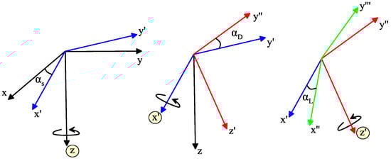
Figure 1.
Rotation matrix of anisotropic resistivity tensor.
The continuity equation for the current density still holds in the anisotropic, where the conductivity tensor’s non-diagonal elements can change the current density’s direction concerning the electric field [18,19]. Expanding the electromagnetic components in Equation (1), constraining and replacing the right term with the full tensor yields the following:
Equations (3) and (4) can be simplified into the second-order partial differential equations containing only and :
Equation (5) is essentially just the individual components of the second-order curl-curl equation projected into 2D with the assumption , including the E-polarization mode of the electric field (TE mode) and the H-polarization mode of the magnetic field (TM mode), where . This is discretized to form the coefficient matrix by staggering the order of the electrical indices on the grid and using the differential and appropriate averaging operators for approximation [19]. Boundary conditions are added to consider the ill-posed problem. The internal assumption of the model is the permeability under vacuum. The internal electric and magnetic components of the boundary are continuous, and the external Dirichlet boundary conditions can be given. To ensure sufficient attenuation of the induced secondary field at the top boundary, the air layer with low conductivity is placed on the top of the model. The permutation equations contain coefficients and node information, and the underground electric and magnetic components are obtained by solving the partial differential problem with the finite difference method.
2.2. Phase Tensor
In MT surveys, the inhomogeneity of the subsurface near conductivity distorts the electromagnetic signal of the underlying or deep conductivity structure. As the signal frequency decreases, the inductive effect by the near-surface structure gradually decreases and becomes negligible compared with the conductive response [20]. This phenomenon is known as electric field distortion. Eliminating the effect of electric field distortion can effectively recover the accurate electrical response of the subsurface structure. Caldwell (2004) proposed the phase tensor (PT) instead of the original swift method [21]. Taking the ratio between the real and imaginary part of the impedance tensor, such that
where is the phase full tensor,
can be expressed as a singular value decomposition of the rotation matrix multiplication in the form
where is the rotation matrix, and are the maximum and minimum values of the coordinate invariants, and the angles and have transformation processes concerning the full tensor and diagonal symmetry. Formally,
where angle β and α are the rotation of the phase tensor asymmetry, and the three coordinate invariants define the phase tensor. Equation (9) has the same form as a square matrix’s singular value decomposition (SVD) [22]. Thus, the and (maximum and minimum values) are the singular values of . In general, the tensor invariants algebra is represented by trace, skew, and determinant:
The invariant is expressed as a first-order function,
where the maximum, minimum, and skew are
Graphically, we may use an ellipse to represent the second-rank phase tensor (Figure 2) [23], where (X1, X2) is defined as the reference coordinate system of the tensor. The tensor principal axis is the major and minor axes of the ellipse, and the angle is the major axis orientation, where the phase tensor is symmetric , and the major axis orientation is given by . Heise et al. introduced the residual phase tensor (RPT) by combining the tensor information from two MT datasets to obtain the difference matrix [24].
where is the identity matrix, is the pre-injection PT, and is the post-injection PT. Calculating the three rotational invariants of , , and can indicate the change of the preferred transport direction of the current [11,25].
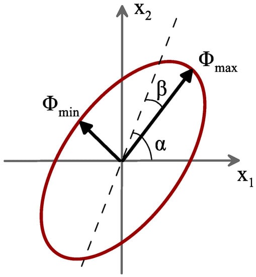
Figure 2.
Construction of a phase ellipse.
3. Phase Tensor to HDR Reservoir Model Testing
This section uses typical HDR reservoir models to simulate the fracture isotropic and anisotropic characteristics by the MT resistivity and phase tensor response. The electrical structural state of the injection process is discussed by simulating fractures containing high conductivity layers to demonstrate that fracture distribution is closely related to electrical anisotropy.
The first HDR reservoir isotropic layer mode is shown in Figure 3, in which the model depth is 15 km, the background resistivity is 1000 Ω·m, and there is a high conductivity layer of 20 Ω·m. (x, y, z) in the MT measurement coordinate system. The impedance tensor is obtained by MT simulation and expressed as a second-order matrix with a non-diagonal equal. The results show that a unit circle represents PT. The primary and minor axis of the ellipse is elongated at 0.1 Hz due to the difference in electrical structure, and the primary axis value is positively correlated with the conductivity. The MT response propagated to the deeper part and the axes narrowed, indicating no structural changes.
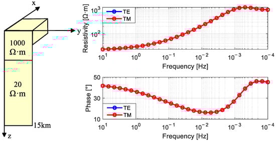
Figure 3.
Isotropic layer model, apparent resistivity, and phase tensor results.
Figure 4 shows the anisotropic layered model with the inclusion of angular deviations. There are different resistivity and angle variations along the electrical axis, Ω·m, 1000 Ω·m. The isotropic layer produces a unit circle change with PT response. However, the elliptical shape shows an increase in the major axis and the angle change when passing through the mutation layer. The high conductivity difference in the x-axis is more sensitive than in the y-axis, so the TE mode has a higher apparent resistivity than the TM. Because of the angle change in y and z directions, electromagnetism is no longer parallel. The phase difference produces an anomaly greater than 45°, making the PT deviate from the central axis.
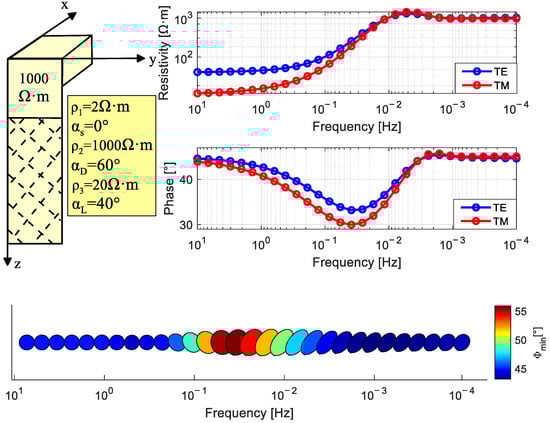
Figure 4.
Anisotropic layered model, apparent resistivity, and phase tensor results.
The results show that the TM and TE modes’ phases and apparent resistivity curves overlap in isotropic layer media. The angular information about fracture distribution can not be observed. The deviation of the electrical axis in the anisotropic model causes the difference in the MT signals, and the TE and TM lag phases have been shown to contain much information related to the electrical angle of the formation. Therefore, using isotropic modelling will overestimate the measurement results. Perkor summarized that the anisotropy characteristics of MT data should be considered in most cases [11].
In Figure 5, an anisotropic layer is embedded into the isotropic space to simulate the fracture distribution. The response in the short period is mainly influenced by the isotropic layer, shown as a unit circle. As the period increases, the fracture produces structural differences, and the change in y-direction decreases the apparent resistivity, as indicated by the increased phase central axis. In addition, the TE is affected by the resistivity in the x-direction, and the phase remains constant. The central axis is larger than the minor axis and points in the y-direction. In low frequency, the interface anomaly no longer affects the surrounding electromagnetic, and the PT returns to the isotropic response. In the anisotropic model, the PT of TM and TE can effectively obtain critical information related to the angle of fracture distribution.
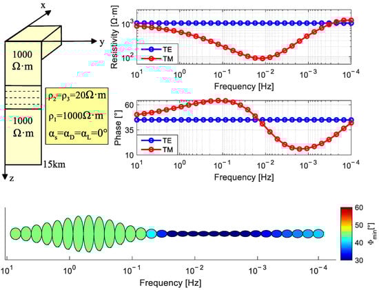
Figure 5.
Interlayer anisotropy media, apparent resistivity, and phase tensor results.
4. Residual Phase Tensor HDR Fracture Monitoring
The PT method depends on electrical interface changes, and the complex structure caused by fractures misjudges the data. The residual PT monitors the moments before and after water injection and can capture a series of parameters such as the direction of fracture distribution and fluid-related electrical characteristics.
4.1. Isotropy Conductivity Change Caused by Water Injection
Figure 6 shows a simplified model of the subsurface with a depth of 15 km, and the low resistivity presence at 3 km indicated the fracture. The background resistivity is 1000 Ω·m, and the fracture is changed by water injection, showing 200 Ω·m, 150 Ω·m, 100 Ω·m, and 50 Ω·m with time, which does not produce anisotropy. The results show that the residual PT is circular, and the color is expressed as the product of the major and minor axes. The decrease in resistivity indicates that fluid is being injected into the subsurface. Since there is no rotation and change of the electrical axis in any direction, the ellipse axes are equal and elongate with the increase of conductivity. The PT response corresponding to 3 km can be monitored from 0.1 Hz to 1 Hz, which indicates that the residual PT method is sensitive to the conductivity changes caused by water injection.
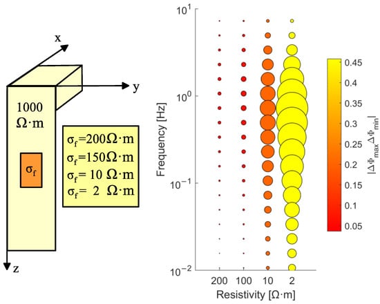
Figure 6.
Fracture isotropic model and residual phase tensor results.
4.2. Effect of Anisotropic on the Residual Phase Tensor
Figure 7 shows the PT response by varying the resistivity in the three electrical axes orientations. The fracture resistivity with 3 km depth is equal to 10 Ω·m in the x, y, and z orientations, respectively. The resistivity in the other orientation is 50 Ω·m.
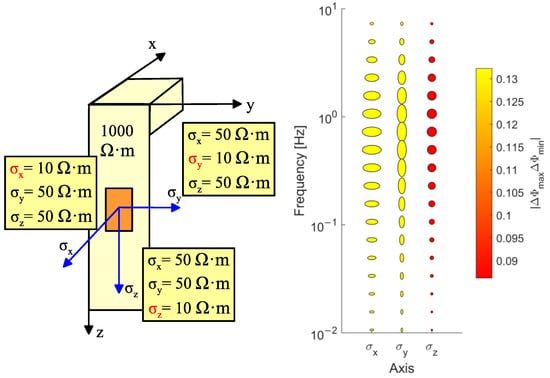
Figure 7.
Fracture anisotropy model and the residual phase tensor with the change of the conductivity axis.
The residual PT method allows the acquisition of the maximum electrical axis in the fracture (Figure 7). The fracture shows an anisotropic resistivity response in a certain axis direction during water injection. The PT of the x and y axes are elliptically distributed from 0.1 to 10 Hz, and the major axis points to 0° and 90° of the rotation coordinates. The vertical axis anomaly cannot respond to the PT because the electromagnetic component is insensitive to the z-axis.
Figure 8 shows the effect of depth on the residual PT. In the background resistivity of 1000 Ω·m, the fractures are buried at a depth of 2 km to 5 km, and the fractures develop in the X direction.
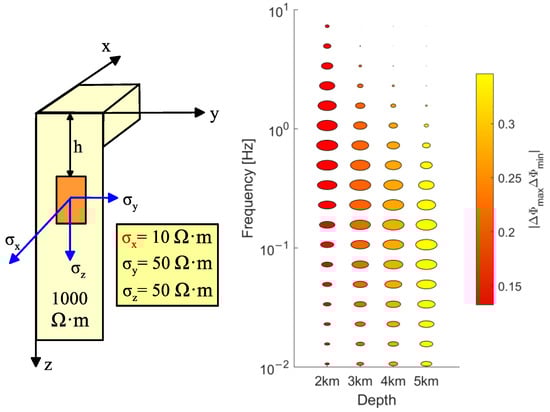
Figure 8.
Fracture anisotropy model and the residual phase tensor with the change of the depth.
The fractures with different depths can still respond to the residual PT, and the maximum electrical axis in the X direction can be observed. Along with the increase of the depth of the anomaly, the frequency of MT signal will decrease, and the resolution of anomaly characterization will also decrease. This is reflected in the attribute color value of the observation ellipse.
Different strokes are also sensitive to the response of residual PT. Figure 9 shows the anisotropic model, considering the change in the direction of the x and y axes. For all modelled scenarios presented in Figure 10 and Figure 11, an observable relationship exists between the strike and the ellipse orientation, which causes the ellipse’s long axis to orientate itself parallel to the anisotropy strike. Note that with the increase of the strike, the ellipse’s major axis shortens, and the minor axis extends. When the strike angle is 45°, the circle phase has the maximum attribute color, and the residual PT cannot distinguish the ellipse deviation angle. There is the same phenomenon on the 45° of the y-axis. This is because the rotation matrix assimilates the anisotropic difference in the horizontal direction, where the major and minor axes are equal at 45°. The y-axis variation has the same characteristics as the x-axis, indicating that the residual PT ellipse possesses an observed response from 0 to 180°. The ellipse axes were normalized to visualize all observations using the peacock method, highlighting the angular information [14]. The 45° strike angle change is observed in the figure on the right, indicating that the original strike is included in the ellipse calculation.
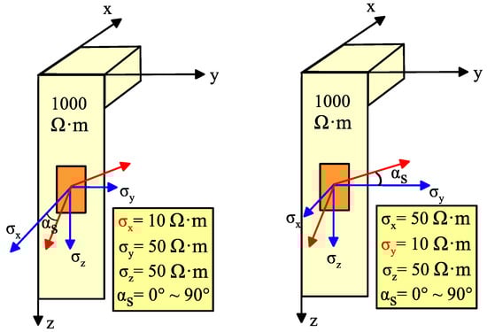
Figure 9.
Fracture anisotropy model with strike variation.
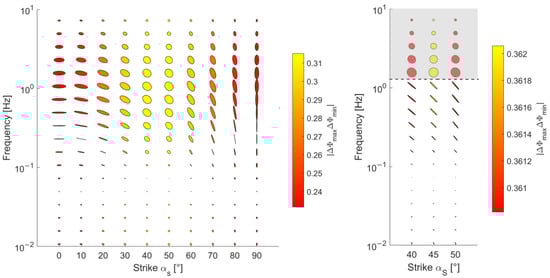
Figure 10.
The residual phase tensor for different strike angles of the conductivity x-axis.
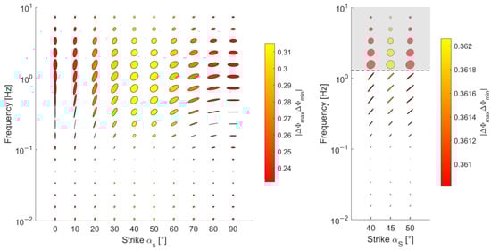
Figure 11.
The residual phase tensor for different strike angles of the conductivity y-axis.
In further analysis of the sensitivity of the dip angle to the residual PT method, when rotating the x-axis, the y-axis has the maximum resistivity (Figure 12). The phase of 0° is elliptical, the increase of dip angle gradually decreases the conductivity response of the y-axis, and the major axis is shortened and shows a circular. Phase attribute color decreases with increasing dip angle. Note that it is not normalized, because the ellipse axes are independent of the strike angle variation but contain as much information as possible about the dip angle. Figure 13 shows the dip rotation at a strike of 30°, which is consistent with Figure 12. The above result shows that the dip does not affect the change in the strike but changes the ellipse axis.
Figure 12.
The fracture anisotropy model and the residual phase tensor for different dip angles in the conductivity y-axis.
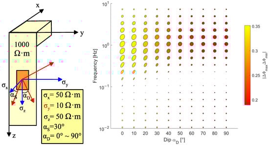
Figure 13.
The fracture anisotropy model and the residual phase tensor for different dip angles in the 30° strike angles.
4.3. Time-Lapse Residual PT Monitoring of Fractured HDR Reservoirs
In this section, other characteristics of the residual PT are analyzed jointly using the coupled field conversion to conductivity model with the addition of a reasonable anisotropic rotation. First, we simulated the coupled injection underground field, and obtained the temperature and pressure distribution for 60 months. The model size is 1 km × 2 km, with intersecting fracture network inside (5th year results in Figure 14). The water injection point is located at 1 km, and 20 °C water is continuously injected at an injection rate of 20 m3/h. As temperature and water saturation affect the conductivity, empirical formulas were used to obtain electrical parameters and calculate MT response (Figure 14). For the specific work details of this part, please refer to Bai et al. [26].
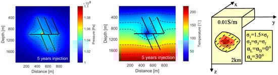
Figure 14.
Coupled field model of temperature, pressure, and conductivity after 5 years of injection.
Add the anisotropy change of 30° strike to the formation after water injection to obtain the residual PT (Figure 15). Electrical structure changes and elliptical deviations of 23 to 32° were monitored at 100 Hz. This indicates the anisotropy development, which coincides with the fracture angle caused by injection.
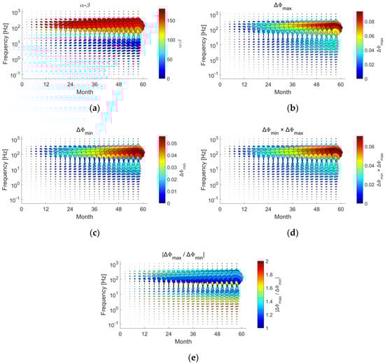
Figure 15.
The time-lapse residual phase tensor, where the colors indicate the combined invariants; (a) ; (b) ; (c) ; (d) and (e) .
The phase ellipse has three invariants and adding attribute colors can display more feature information, including the major, minor axis, and ellipse angle. The value is the rotational of the ellipse, which is directly related to the anisotropic axis or the electric field distortion axis. and is the scalar value of ellipse axis, which represents the dimensional change of electrical structure. The ellipse color away from the injection becomes lighter, indicating that the electrical difference decreases. Generally, the horizontal anisotropy is related to the ellipse axes. When the conductivity increases, the major and minor axes elongate.
and are combined invariants. Previous work defines the former as having the information of structure, and the multiplication of ellipse axes can represent the comprehensive characteristics of horizontal anisotropy. The latter is defined as the elliptic flat invariants or the variance in subsurface horizontal anisotropy. When is larger, it means that the difference in the conductivity axes is more prominent. In the isotropic, .
5. Discussion
The calculation of the PT is essential for solving different anisotropic, correcting electric distortions, and monitoring the subsurface time-lapse distribution. The PT variation response and subsurface structure can provide evidence for subsequent HDR monitoring. The residual PT uses the MT at different moments to calculate the difference, effectively eliminating the natural frequency and regular noise during the survey and monitoring the anisotropic angle of fractures caused by injection. This method has a good application in the time-lapse monitoring of MT. This paper discusses the sensitivity of PT to anisotropy and its application in HDR fracture systems in detail through the model test.
In conclusion on the results, the electrical variation in the subsurface was generally reflected in the anisotropic or isotropic change. The difference lay in the inequality or equality of the three conductivity axes (x, y, z). The residual PT was circular for isotropic media, which was proportional to the ellipse axes. Anisotropic media caused elliptical changes, with the major axis pointing to the maximum conductivity axis. Note that residual PT was sensitive to the horizontal axis (x,y), while the vertical axis (z) had no resolution. The more significant the difference in horizontal anisotropy, the flatter the ellipse.
Generally, there was an angle difference between the subsurface anisotropy and the surface measurement system, which indicated that the MT survey lines were not aligned with the conductivity axis. A rotation matrix was applied to transform the conductivity tensor to obtain the dataset in the measurement system. Figure 16 shows the sensitivity analysis of the change in the strike to the residual PT, where the curves indicate the ratio of the major axis to the minor axis. Here, suggests that the phase is elliptical, and the strike can be observed. Tests found that the residual PT had angular sensitivity over a range of horizontal variations from 0 to 180°. An angle greater than 180° was considered to produce a rotation. The residual PT makes an isotropic response when the survey system differs from the conductivity axis by 45° or 135°, showing a circle with equal ellipse axes. This phenomenon can be solved by normalization.
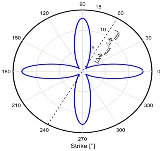
Figure 16.
Sensitivity analysis of the strike angle of the injection fracture model to the residual phase tensor.
There are strict assumptions on the response of the dip angle to the MT. Figure 17 shows the sensitivity analysis of the change in the dip to the residual PT. When the survey line is parallel to the axis of maximum anisotropy and is rotated along it, the major axis of the PT does not produce a response. The major axis records the rotating axis coinciding with the maximum anisotropy axis. In contrast, the change of the minor axis depends on the joint action of another horizontal axis and vertical axis. Dip changes are also sensitive to residual PT. In Figure 17, when , the major ellipse axis shortens as the tendency angle increases. When , the major axis elongates. Note that the dip changes do not produce a deviation from the elliptical orientation.
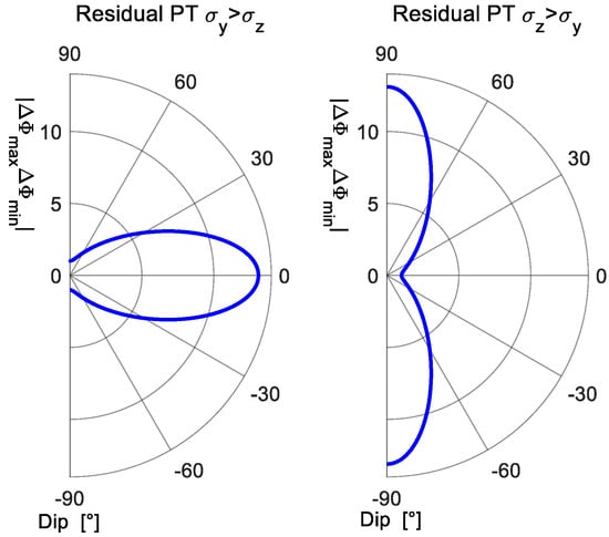
Figure 17.
Sensitivity analysis of the dip angle of the injection fracture model to the residual phase tensor.
The HDR monitoring needs to consider the MT data before injection as a reference background for the residual PT to obtain critical information about fracture distribution and subsurface structural changes by observing MT after injection. The selection of reference data is crucial, which may be accompanied by an anisotropic electrical structure unrelated to fracture. Figure 18 shows the response of the residual PT when considering the anisotropic in the subsurface before injection. Assuming that the background possesses a low conductivity before injection, the maximum electrical distribution exists along the horizontal axes. The model after the injection has the same parameter settings as in Figure 9. The results show that anisotropic background affects the residual PT after injection. When the strike coincides with the maximum horizontal axis, the will be smaller than the anisotropic (Figure 16). This can be explained by the decrease in the phase difference between the two moments. However, the fracture strike can still be observed in the results.
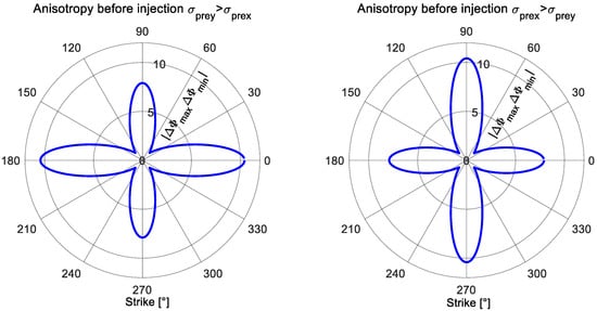
Figure 18.
Sensitivity analysis of the anisotropy model before injection to the residual phase tensor.
6. Summary
This paper presents the numerical simulation study of HDR fracture time-lapse monitoring based on the anisotropic MT method. Typical model test results demonstrate that the residual PT can obtain reliable results in the injection process. The sensitivity and response characteristics of the residual PT are discussed in detail by testing the fracture model with different depths and parameters and calculating the time-lapse of the coupling field. The PT ellipse axes and angles are related to the subsurface conductivity and anisotropy angle, respectively. Compared with other geophysical methods, MT can indirectly interpret the distribution of fractures caused by the subsurface injection and critical characterization, such as development direction and dip angle, providing a technical means for the exploitation and subsequent evaluation of HDR geothermal. In the future, 3D-modelling and measured data will be studied to obtain actual site results, providing a basis for geothermal fracturing.
Author Contributions
Conceptualization, J.L. and L.B.; methodology, L.B. and J.L.; software, L.B.; validation, J.L., L.B. and Z.Z.; formal analysis, J.L.; investigation, J.L.; resources, L.B.; data curation, L.B. and J.L.; writing—original draft preparation, L.B.; writing—review and editing, J.L. and Z.Z.; visualization, L.B.; supervision, J.L.; project administration, J.L.; funding acquisition, J.L. All authors have read and agreed to the published version of the manuscript.
Funding
This work is supported by the Natural Science Foundation of China (41874134, 4207040044 and 42174065) and the Youth Talent Project of the China Association for Science and Technology (2019QNRC001).
Data Availability Statement
Not applicable.
Acknowledgments
The authors would like to thank the editors and reviewers for their valuable comments and suggestions that greatly improve our manuscript, as well as MacFarlane for his theoretical help.
Conflicts of Interest
The authors declare no conflict of interest.
References
- Wang, G.L.; Zhang, W.; Ma, F.; Lin, W.J.; Liang, J.Y.; Zhu, X. Overview on hydrothermal and hot dry rock researches in China. China Geol. 2018, 1, 273–285. [Google Scholar] [CrossRef]
- Bertani, R. Geothermal power generation in the world 2005–2010 update report. Geothermics 2012, 41, 1–29. [Google Scholar] [CrossRef]
- MacFarlane, J.; Thiel, S.; Pek, J.; Peacock, J.; Heinson, G. Characterisation of induced fracture networks within an enhanced geothermal system using anisotropic electromagnetic modelling. J. Volcanol. Geotherm. Res. 2014, 288, 1–7. [Google Scholar] [CrossRef]
- House, L. Locating microearthquakes induced by hydraulic fracturing in crystalline rock. Geophys. Res. Lett. 1987, 14, 919–921. [Google Scholar] [CrossRef]
- Albaric, J.; Oye, V.; Langet, N.; Hasting, M.; Lecomte, I.; Iranpour, K.; Messeiller, M.; Reid, P. Monitoring of induced seismicity during the first geothermal reservoir stimulation at Paralana, Australia. Geothermics 2014, 52, 120–131. [Google Scholar] [CrossRef]
- Newman, G.A.; Gasperikova, E.; Hoversten, G.M.; Wannamaker, P.E. Three-dimensional magnetotelluric characterization of the Coso geothermal field. Geothermics 2008, 37, 369–399. [Google Scholar] [CrossRef]
- Didana, Y.L.; Heinson, G.; Thiel, S.; Krieger, L. Magnetotelluric monitoring of permeability enhancement at enhanced geothermal system project. Geothermics 2017, 66, 23–38. [Google Scholar] [CrossRef]
- Carbonari, R.; Di Maio, R.; Piegari, E. Feasibility to use continuous magnetotelluric observations for monitoring hydrothermal activity. Numerical modeling applied to campi flegrei volcanic system (Southern Italy). Front. Earth Sci. 2019, 7, 13. [Google Scholar] [CrossRef]
- Kellett, R.L.; Mareschal, M.; Kurtz, R.D. A model of lower crustal electrical anisotropy for the pontiac subprovince of the canadian shield. Geophys. J. Int. 1992, 111, 141–150. [Google Scholar] [CrossRef]
- Heise, W.; Caldwell, T.G.; Bibby, H.M.; Brown, C. Anisotropy and phase splits in magnetotellurics. Phys. Earth Planet. Inter. 2006, 158, 107–121. [Google Scholar] [CrossRef]
- Peacock, J.R.; Thiel, S.; Heinson, G.S.; Reid, P. Time-lapse magnetotelluric monitoring of an enhanced geothermal system. Geophysics 2013, 78, B121–B130. [Google Scholar] [CrossRef]
- Abdelfettah, Y.; Sailhac, P.; Larnier, H.; Matthey, P.D.; Schill, E. Continuous and time-lapse magnetotelluric monitoring of low volume injection at Rittershoffen geothermal project, northern Alsace-France. Geothermics 2018, 71, 1–11. [Google Scholar] [CrossRef]
- Rosas-Carbajal, M.; Linde, N.; Peacock, J.; Zyserman, F.I.; Kalscheuer, T.; Thiel, S. Probabilistic 3-D time-lapse inversion of magnetotelluric data: Application to an enhanced geothermal system. Geophys. J. Int. 2015, 203, 1946–1960. [Google Scholar] [CrossRef]
- Peacock, J.R.; Thiel, S.; Reid, P.; Heinson, G. Magnetotelluric monitoring of a fluid injection: Example from an enhanced geothermal system. Geophys. Res. Lett. 2012, 39, 5. [Google Scholar] [CrossRef]
- Vozoff, K. Magnetotellurics—principles and practice. Proc. Indian Acad. Sci.-Earth Planet. Sci 1990, 99, 441–471. [Google Scholar] [CrossRef]
- Price, A.T. Theory of magnetotelluric methods when source field is considered. J. Geophys. Res. 1962, 67, 1907–1918. [Google Scholar] [CrossRef]
- Pek, J.; Santos, F.A.M. Magnetotelluric impedances and parametric sensitivities for 1-D anisotropic layered media. Comput. Geosci. 2002, 28, 939–950. [Google Scholar] [CrossRef]
- Weidelt, P. 3-D conductivity models: Implications of electrical anisotropy. In Three-Dimensional Electromagnetics; Society of Exploration Geophysicists: Houston, TX, USA; pp. 119–137.
- Guo, Z.Q.; Egbert, G.D.; Wei, W.B. Modular implementation of magnetotelluric 2D forward modeling with general anisotropy. Comput. Geosci. 2018, 118, 27–38. [Google Scholar] [CrossRef]
- Jiracek, G.R. Near-surface and topographic distortions in electromagnetic induction. Surv. Geophys. 1990, 11, 163–203. [Google Scholar] [CrossRef]
- Caldwell, T.G.; Bibby, H.M.; Brown, C. The magnetotelluric phase tensor. Geophys. J. Int. 2004, 158, 457–469. [Google Scholar] [CrossRef]
- Press, W.H. Numerical Recipes in C++: The Art of Scientific Computing, 2nd ed.; (C++ ed., Print. is Corrected to Software Version 2.10); Cambridge University Press: Cambridge, UK, 1992. [Google Scholar]
- Bibby, H.M. Analysis of multiple-source bipole-quadripole resistivity surveys using the apparent resistivity tensor. Geophysics 1986, 51, 972–983. [Google Scholar] [CrossRef]
- Heise, W.; Bibby, H.M.; Caldwell, G.; Bannister, S.C.; Ogawa, Y.; Takakura, S.; Uchida, T. Melt distribution beneath a young continental rift: The Taupo Volcanic Zone, New Zealand. Geophys. Res. Lett. 2007, 34, 6. [Google Scholar] [CrossRef]
- Macfarlane, J. Anisotropic Forward Modelling of Fluid Injection and Phase Angles Exceeding 90° in Magnetotellurics. Ph.D. Thesis, University of Adelaide, Adelaide, Australia, 2012. [Google Scholar]
- Lige, B. Time-Lapse Geophysical Monitoring and Deep Learning Prediction of Hot Dry Rock Reservoir. Master’s Thesis, Jilin University, Changchun, China, 2022. [Google Scholar]
Publisher’s Note: MDPI stays neutral with regard to jurisdictional claims in published maps and institutional affiliations. |
© 2022 by the authors. Licensee MDPI, Basel, Switzerland. This article is an open access article distributed under the terms and conditions of the Creative Commons Attribution (CC BY) license (https://creativecommons.org/licenses/by/4.0/).