Development of a Flashover Voltage Prediction Model with the Pollution and Conductivity as Factors Using the Response Surface Methodology

Abstract

In this paper, the response surface methodology (RSM) is used to predict the flashover voltage of a cap and pin 1512L insulator used by SONELGAZ Algerian Power Company (SPE). The pollution and conductivity are studied using a two-level central composite design. MINITAB 19 software is used to perform the regression analysis and analysis of variance (ANOVA) of the data, from which the full quadratic model is developed. The results show that both the pollution and conductivity have a significant effect on the response. The model validation shows the good agreement between the experiment’s obtained results and the predicted results. Therefore, the model could be used to predict the flashover voltage.

1. Introduction

High-voltage outdoor insulators are essential parts of transmission lines. One of their prime constraints is pollution [1,2,3,4,5,6]. Under dry conditions, the pollution allows for a small leakage current to pass, although in the presence of light rain, fog or dew the surface becomes highly conductive, which may lead to a flashover [1,2,3,4,5,6,7,8,9,10,11,12,13,14,15]. The reason for this is that after the pollution becomes wet, its presence leads to an increase in the leakage current along with the dry band widening. Therefore, it is safe to say that the flashover phenomenon due to pollution of the insulator follows a defined mechanism. First is the accumulation of the pollution on the surface of the insulator. Secondly, this polluted surface becomes more moisturized. Thirdly, an increase in the value of the leakage current will occur. Lastly, the flashover manifests along the surface of the insulator through the polluted areas [16].

With time and with the insulator under these conditions, the insulator’s surface characteristics may undergo some changes that might lead to premature aging [17].One of the first models to be proposed for contamination flashover was the Obenaus model, consisting of a discharging space in series with a resistance. The discharge and the pollution resistance represent the arc bridging the dry band and the unbridged portion of the insulator, respectively [18]. Many researchers have based their research and studies on this model, such as the Claverie model, which is described as a relationship between the minimum arc re-ignition voltage U_cx and the arc current I [19]. Neumarker’s model is a modified version of the Obenaus model using the uniform resistance per unit length instead of a fixed resistance [20]. Despite the many experiments and studies that have been performed, the flashover phenomenon is still a complex topic that must be understood in order to understand the process leading to the flashover under polluted conditions [21].Throughout the years of research, researchers have used different methods to predict the flashover phenomena. Using statistical methods, numerous predictions about the flashover phenomena have been made. While investigating the predictions made by different author, Venkataraman and Gorur [18] reported that for traditional porcelain and glass insulators, the predictions had a different range of values, which indicated the poor understanding of the flashover process. The least squares support vector machines approach has shown the ability to create a model by obtaining the relationship between the critical flashover voltage (FOV) and input variables, such as the insulator height, insulator diameter, leakage length of the insulator for an element, surface conductivity, number of elements on a chain, and number of shed and predict values of the critical flashover voltage that are not used in the training stage accurately [22]. For variables such as the pollution conductivity and pollution quantities and using an artificial neural network, Bourek et al. [23] found that there was a similarity between the results obtained and the practical results. The response surface methodology (RSM) and analysis of variance (ANOVA) are methods used hand-in-hand to build, analyze, and prove the accuracy of a model. Zhao et al. [24] developed a new least squares support vector machine (LS–SVM) model that was proposed to predict the flashover voltage (FOV).The model is acceptable for predicting the FOV values of composite insulators. Cui et al. [25] evaluated the flashover performance using statistical methods applied to composite and ceramic insulators. The results improved the flashover performance to acceptable levels. The RSM is a mix of statistical and mathematical techniques that is used for planning experiments, analysis, and model building [26,27,28]. This method allows the study and observation of two or more variables simultaneously [28,29] while determining the relationship between these variables and the response [30]. ANOVA is used to check the precision of the built model.

Too few papers have been reported regarding the prediction of the flashover voltage values of insulators using the response surface design. The purpose of the present paper is to develop a mathematical model that can predict the flashover voltage of a cap and pin 1512L insulator. With the aid of MINITAB 19 software, the central composite design is used to develop a model that can predict the flashover voltage using two factors, the pollution and conductivity.

The rest of the paper is organized as follows. Section 2 provides a brief description of the real model of the insulator, the mathematical model, and the model we are working for the central composite design of response surfaces. In Section 3, the numerical results (fits, diagnostics, surface, contour plot, and confirmation with the real model of an insulator) using the Minitab software are presented and discussed. Finally, the conclusions of the present work are drawn.

2. Design Setup

The experimental domain was the field that the results of the study were based on, so care was taken to obtain the desired results. The results are most valid for the range of values of the factors selected here. The factors of our study were taken from an experiment performed by Benguesmia et al. [1]; the pollution levels that were chosen by [1] were used so as to create several voltage levels for each conductivity value in order to better understand the phenomenon of circumvention and to observe clean, less-polluted, and fully polluted scenarios (for each conductivity value, we created eight levels of pollution). While most of the models previously created by researchers deal with the leakage current as a factor, we took a different approach, since the leakage current appears after the increase in the dry band’s surface along with the increases in conductivity, meaning the leakage current starts to appear and increase as the previously mentioned conditions are met. As the leakage current increases, this eventually leads to the appearance of the flashover voltage, so we simply bypassed the measurement of the leakage current, making the model less complicated.

The values of the factors and range of the experimental design are shown in

Table 1. Values of the factors studied.

Factors	Level of Pollution (L)	Conductivities (mS/cm)
Level −1	2	1.823
Level 0	5	16.1615
Level 1	8	30.50

. The level of pollution is represented in Figure 1 below.

The mathematical model that represents our study is given as Equation (1). The model we are working with is the central composite design of the response surfaces. Central composite designs are designs with center points, augmented with a group of axial points that lets the curvature be estimated. They can be used to estimate the first- and second-order terms. The relationship between the response and the variables can be represented with a second-degree quadratic equation.

Here, X is the matrix experiment and y is the flashover voltage (the response). The number of unknown parameters (β_i) and the polynomial determined from the model are given by the following equation:

$$y={\beta }_0 +{\displaystyle \sum _{i=1}^k{\beta }_i X_i+{\displaystyle \sum _{i=1}^{k-1}{\displaystyle \sum _{j=i+1}^k{\beta }_{ij} X_i X_j+{\displaystyle \sum _{i=1}^k{\beta }_{ii} X_i^2}}}}$$

(1)

$$y={\beta }_0+{\beta }_1 x_1+{\beta }_2 x_2+{\beta }_{12} x_{12}+{\beta }_{11} x_1^2+{\beta }_{22} x_1^2$$

(2)

This design consists of the nine runs represented in

Table 2. Central composite design plan for this study.

Number of Experiments	Level of Pollution  (L)	Conductivities σ (mS/cm)	Flashover Voltage  Uc (kV)
1	−1	−1	76.6080
2	1	−1	42.6720
3	−1	1	76.6080
4	1	1	28.7000
5	−1	0	76.6080
6	1	0	34.6333
7	0	−1	50.7360
8	0	1	35.6000
9	0	0	40.9855

, four factorial points, four axial points, and one center point with an alpha value of 1.

3. Results and Discussion

The flashover voltage was predicted using a central composite design. Using MINITAB 19 software, the inputs given in Table 2 were subjected to various regression analyses, and the results are presented in

Table 3. Coded and uncoded coefficients along with the coded t-values of the model.

Terms	Coefficients (Coded)	Coefficients (Uncoded)	t-Value	p-Value
Constant	45.884	73.206	135.76	0.000
L	−6.973	−5.551	−37.67	0.000
σ	−5.711	−0.5462	−30.85	0.000
$\mathrm{L}·\mathsf{\sigma }$	1.422	−0.03306	7.56	0.008
$\mathrm{L}·\mathrm{L}$	2.423	0.2693	−0.35	0.005
$\mathsf{\sigma }·\mathsf{\sigma }$	−0.111	0.00054	6.27	0.753

in coded and uncoded forms, along with the t-values and p-values. The threshold value of the t-value was 3.18, which was obtained through the Student’s T-table by crossing the degrees of freedom of the error and the confidence interval. The purpose of using the t- and p-values was to determine the significance of the coefficients found. For the significance level, we chose α = 0.05 to determine the significant and non-significant terms.

The mathematical equation is written in the following uncoded form:

$$U_c=73.206-5.551 L-0.5462 \sigma -0.03306 L \sigma +0.2693 L^2+0.00054 {\sigma }^2$$

(3)

Here, the higher the t-value, the bigger the effect of the term on the model, and the negative sign indicates that the term has a negative effect on the response. A lower p-value (α ≤ 0.05) indicates the significance of the term on the model, i.e., the response.

The alpha (α) value is the distance of each axial point (also called a star) from the center in a centered composite plane.

The Pareto chart shows the absolute values of the standardized effects from the largest to the smallest effects. While the normal probability plot of the effects shows the relativity, the standardized effects are compared to a distribution fit line when all of the effects equal0.The normal plot of the standardized effects is a linear representation of the probability versus the standardized effects; in other word, it is the probability that any term’s standardized effect will be lower than the given value.

The Pareto chart (Figure 2) shows the magnitude of the terms to help compare their effects on the model in order to see which effect is greater than the others. All of the terms L, σ, L·L, L·σ have a higher value than 3.18, so their effects impact our model, while σ·σ is negligible. Here, L is the term with the most effect and L·σ is the least effective term. The normal plot (Figure 3) shows the effect a term has on the model in a way that the terms that are on the left of the value x = 0 have a negative effect, which means that the more an effect increases the more the response decreases. The effects on the right have a positive effect, which means the more an effect increases the more the response increases. Therefore, the uncoded equation above becomes:

$$U_c=73.206-5.551 L-0.5462 \sigma -0.03306 L \sigma +0.2693 L^2$$

(4)

The fit values (estimated values of the model) are taken for comparison with the experimental ones, and this will show the adequacy of our model. On the (X) axis we have the response, which is the breakdown voltage we obtained from experiments, while on the (Y) axis we have predictor, which is the breakdown voltage we obtained from the equation. The points are aligned along the line y = x, which means that the model is nearly perfect (see Figure 4).

The regression equation was developed between the experimental response and the estimated response using MINITAB. The equation is calculated in the following form:

$$Y={\beta }_0+{\beta }_1 x$$

(5)

while:

$$b_1=\frac{{\displaystyle \sum (x_i-\overline{x}) (y_i-\overline{y})}}{{\displaystyle \sum {(x_i-\overline{x})}^2}}$$

(6)

$$b_0=\overline{y}-b_1 \overline{x}$$

(7)

where y_i is the ithobserved response value, x_i is the ithpredictor value, y is the mean response, and x is the mean predictor, meaning we get:

$$U_{c(\mathrm{model})}=0.0587+0.9988 U_{c(\mathrm{experimental})}$$

(8)

These results show that our model is highly accurate but further analysis of variance results are given to solidify these results.

Table 4. The analysis of variance table.

Source	Degrees of Freedom	Sums of SQUARES	Contribution  %	F-Value	p-Value
Linear	2	487.48	95.97	1185.49	0.0000
Square	2	11.77	2.32	28.62	0.0111
Two-way  interaction	1	8.09	1.59	39.34	0.0082
Error	3	0.62	0.12	//	//
Total	8	507.950	100	//	//

shows the results of the ANOVA, where the p-value is lower than 0.005, which indicates the significance of the terms. The contribution of the error to the model is very low at0.12%. The F-value is similar to the t-value, and both can help find the p-value, so having a higher value means a higher level of significance. In our case, the critical F-value is 4.494 and is found through the F distribution table.

S is measured in units of U_c and represents the difference between the experimental values and the estimated ones. The lower this value is the better. R² is used to determine how well the model fits the data. The adjusted R² tells the factors that are needed in this experiment to obtain these results, so a high value means that they are all needed. The predicted R² tells how well the model predicts the response for new values.

Therefore, the closer these values are to 100% percent the better. Therefore, with the values presented in

Table 5. The summery of the model.

S	R2	Adjusted R2	Predicted R2
0.453433	99.88%	99.68%	98.53%

, we can say for sure that the model is nearly perfect in this study.

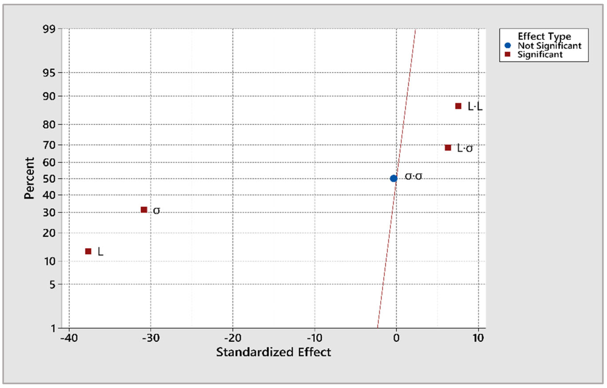
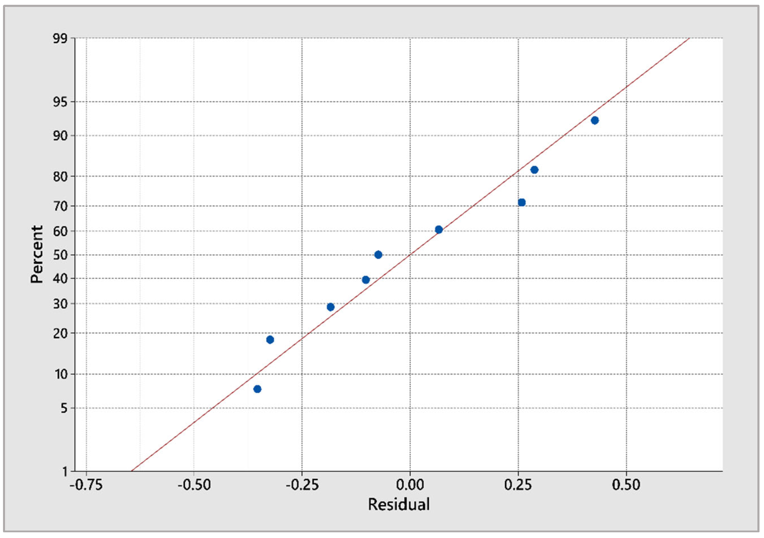
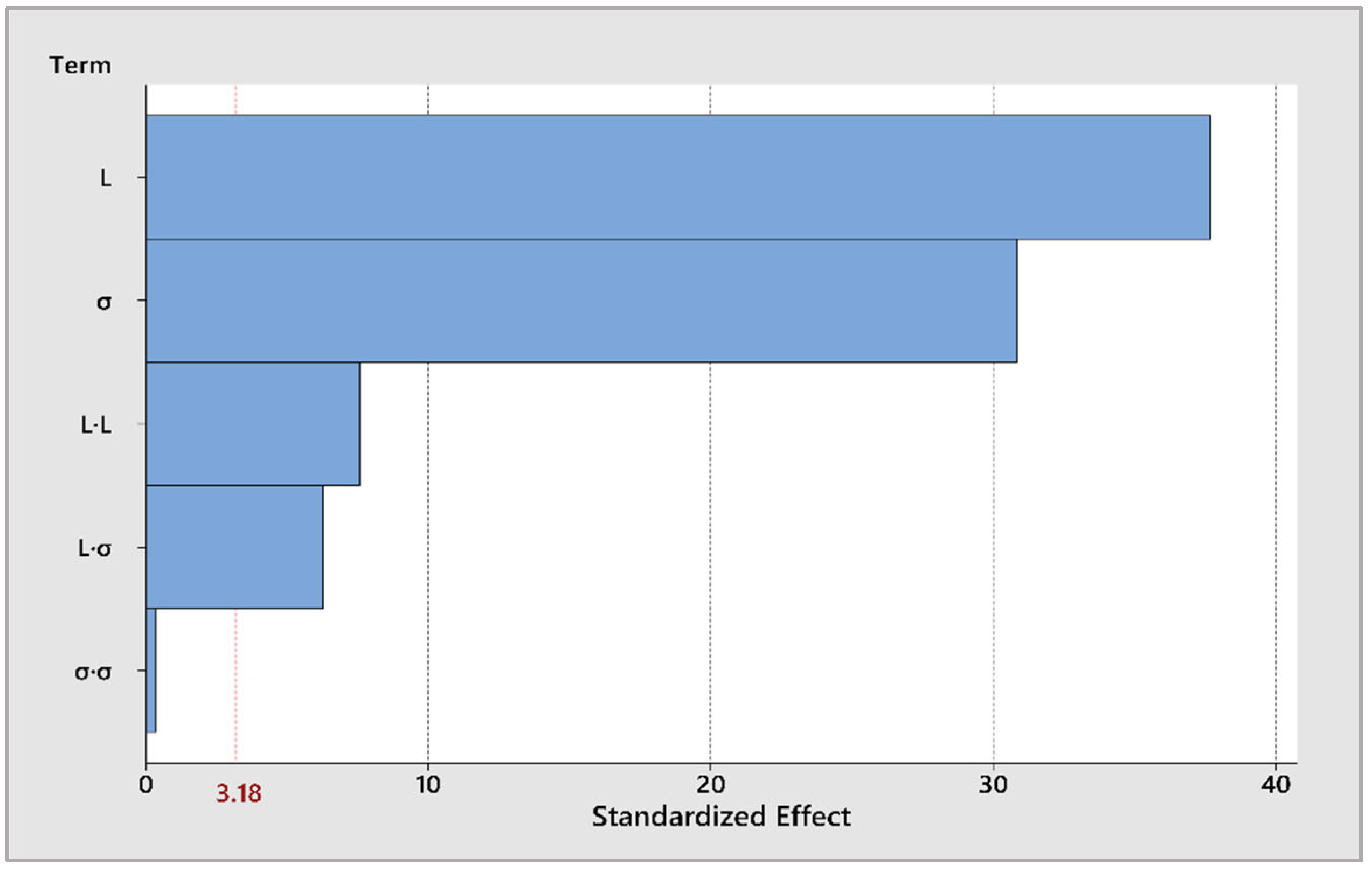
3.1. Fits and Diagnostics

The standard error of the fit, or for short the CI, is used with the t = 3.18 value to calculate the 95% confidence interval:

$$CI=FIT\pm (t=3.18) SE$$

(9)

The results are shown in the

Table 6. Fits and diagnostics for observations.

No	Uc (exp) (kV)	Uc (Model) (Fit)	Standard Error of Fit (SE)	95% Confidence Interval		Residuals
				Lower	Higher
1	62.2	62.303	0.407	61.008	63.598	−0.103
2	45.8	45.513	0.407	44.217	46.808	0.287
3	47.12	48.036	0.407	46.741	49.332	−0.324
4	37	36.934	0.407	35.639	38.229	0.066
5	55.708	55.28	0.338	54.205	56.356	0.427
6	40.98	41.334	0.338	40.258	42.409	−0.354
7	51.3	51.484	0.338	50.409	52.56	−0.184
8	40.32	40.062	0.338	38.986	41.137	0.258
9	45.81	45.884	0.338	44.808	46.959	−0.074

.

To verify the CI results, the normal probability plot is drawn. It displays the residuals versus their expected values when the distribution is normal.

The residuals shown in Figure 5 approximate follow a straight line, which indicates that the assumption that the residuals are normally distributed is verified. With this, we can say that the confidence intervals are more or less accurate. To better see the results, all Uc(exp), fit, and confidence interval values are plotted in Figure 6.

In all nine experiments that were performed, the estimated breakdown voltage was almost equal to the experimental values and the voltages stated by the model, as the confidence interval enclosed the both of them. This shows that the model is accurate with the significance level stated prior.

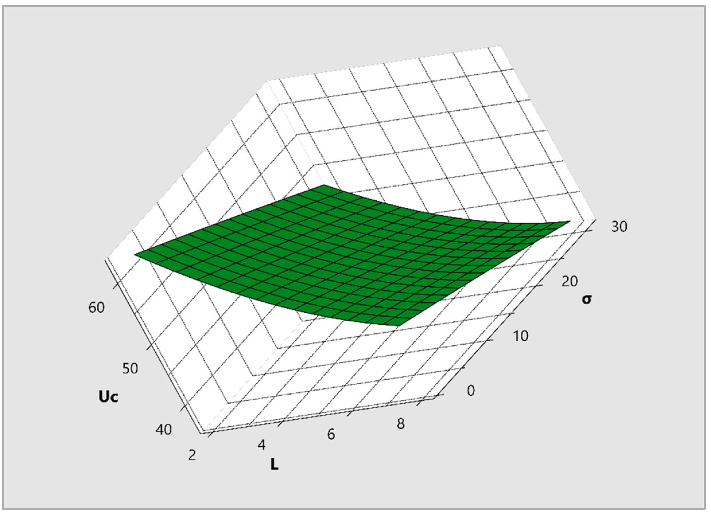
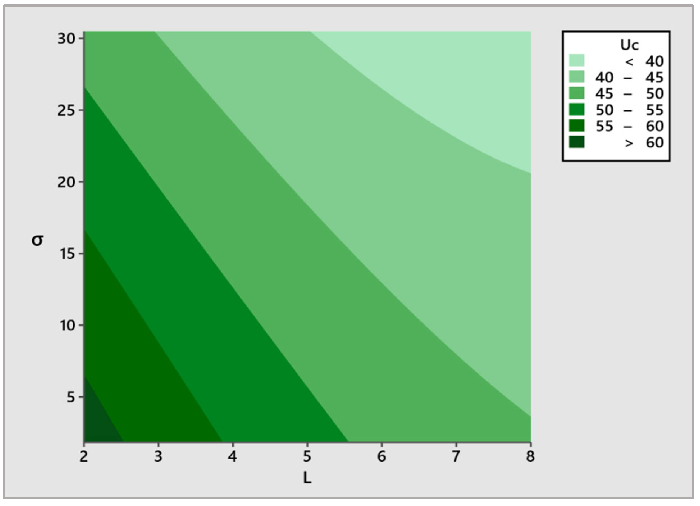
3.2. The Surface and Contour Plots

The mathematical equation is presented graphically in the surface and contour plots.

Both Figure 7 and Figure 8 help us visualize the responses and interactions with the factors better. We can see that both the level of pollution and the value of conductivity have a high effect on the breakdown voltage, such that the increase inone or both will cause a considerable drop in the flashover voltage.

3.3. Further Confirmation of the Model

The table below (

Table 7. Experimental verification data.

Runs	Level of Pollution (L)	Conductivity σ (mS/cm)	Flashover Voltage (Numerical Model) kV	Flashover Voltage ref. [1] kV	Error (%)
2	8	8.02	43.773	42.672	2.58
3	3	1.823	58.162	58	0.28
4	6	30.5	38.986	39.312	−0.83

) shows the results of further experiments with different pollution and conductivity values compared to the results calculated using the model with the different factor values, where by the absolute calculated error range is between 0% and 2.58%, which is very good. From this, we can conclude that the model could predict the flashover voltage with high accuracy.

4. Conclusions

The breakdown voltage of the 1512L insulator was investigated using the design of experiments method. The response surface central composite method was selected to build a model linking the factors, the level of pollution, and its value of conductivity. A total of 9 runs were studied and a high correlation coefficient was found (R² = 99.88%), along with the predicted R² (predicted R² = 98.53%) and a very small standard deviation coefficient (S = 0.453433), indicating that the model fit the data well. The model was made to predict the insulator’s flashover voltage, and the verification data showed that the model was almost perfectly accurate. An adjusted R² equivalent to 99.68% was found, indicating that the model did not contain any unneeded factors.

The simulation and experimental results showed that the increase in one or both factors leads to a decrease in the breakdown voltage. This method showed an incredible level of usefulness by lowering the cost of the study while producing a very good result, showing the accuracy of and different interactions between the factors. One of the purposes of this model is to help engineers in knowing how much the FOV of an insulator is; therefore, by obtaining the data fora certain region (pollution level and the conductivity), engineers can plan the periodic washing or cleaning of pollution from an insulator. In addition, what makes this model stands out is that it is highly precise in predicting the flashover voltage, since it is tailored for and based on a real insulator experiment, along with its simplicity compared to other models.

References

1. Benguesmia, H.; M’ziou, N.; Boubakeur, A. Experimental study of pollution effect on the behavior of high voltage insulators under alternative current. Front. Energy 2021, 15, 213–221. [Google Scholar] [CrossRef]
2. Terrab, H.; Bayadi, A. Experimental study using design of experiment of pollution layer effect on insulator performance taking into account the presence of dry bands. IEEE Trans. Dielectr. Electr. Insul. 2014, 21, 2486–2495. [Google Scholar] [CrossRef]
3. Benguesmia, H.; Bakri, B.; Khadar, S.; Hamrit, F.; M’ziou, N. Experimental study of pollution and simulation on insulators using COMSOL® under AC voltage. Diagnostyka 2019, 20, 21–29. [Google Scholar] [CrossRef]
4. Benguesmia, H. Modeling an Insulator Under Pollution Conditions under Alternative Voltage 50 Hz. Ph.D. Thesis, Biskra University, Biskra, Algeria, 2018. [Google Scholar]
5. M’ziou, N.; Benguesmia, H.; Rahali, H. Modeling Electric Field and Potential Distribution of an Model of Insulator in Two Dimensions by the Finite Element Method. Int. J. Energetica IJECA 2018, 3, 1–5. [Google Scholar] [CrossRef]
6. Benguesmia, H.; M’ziou, N.; Boubakeur, A. AC flashover: An analysis with influence of the pollution, potential and electric field distribution on high voltage insulator. In Multiphysics Modelling and Simulation for Systems Design and Monitoring; Springer International Publishing: Cham, Switzerland, 2015. [Google Scholar] [CrossRef]
7. Ghermoul, O.; Benguesmia, H. Numerical simulation of potential and electric field distribution for contaminated glass insulators. In Advances in Mechanics and Energy, Proceeding of International Conference on Mechanics and Energy (ICME’2021-082), Sousse, Tunisia, 27–29 December 2021; IEEE: Piscataway, NJ, USA, 2021; p. 67. [Google Scholar]
8. Benguesmia, H.; Mechta, A.E.; Ghazal, R. Numerical simulation of potential and electric field distributions on HV Insulators String. In Advances in Mechanics and Energy, Proceeding of International Conference on Mechanics and Energy (ICME’2021-150), Sousse, Tunisia, 27–29 December 2021; IEEE: Piscataway, NJ, USA, 2021; p. 74. [Google Scholar]
9. Diaz-Acevedo, J.A.; Escobar, A.; Grisales-Noreña, L.F. Optimization of corona ring for 230 kV polymeric insulator based on finite element method and PSO algorithm. Electr. Power Syst. Res. 2021, 201, 107521. [Google Scholar] [CrossRef]
10. Khatoon, S.; Khan, A.A.; Tariq, M.; Alamri, B.; Mihet-Popa, L. Flashover Voltage Prediction Models under Agricultural and Biological Contaminant Conditions on Insulators. Energies 2022, 15, 1297. [Google Scholar] [CrossRef]
11. Hassan, E.; Nasrat, L.; Kamel, S. Experimental and Estimation of Flashover Voltage of Outdoor High Voltage Insulators with Silica Filler Based on Grey Wolf Optimizer. Int. J. Emerg. Electr. Power Syst. 2019, 20, 20190035. [Google Scholar] [CrossRef]
12. Benguesmia, H.; M’ziou, N.; Boubakeur, A. Simulation of the potential and electric field distribution on high voltage insulator using the finite element method. Diagnostyka 2018, 19, 41–52. [Google Scholar] [CrossRef]
13. Salem, A.A.; Abd-Rahman, R.; Rahiman, W.; Al-Gailani, S.A.; Al-Ameri, S.M.; Ishak, M.T.; Sheikh, U.U. Pollution Flashover Under Different Contamination Profiles on High Voltage Insulator: Numerical and Experiment Investigation. IEEE Access 2021, 9, 37800–37812. [Google Scholar] [CrossRef]
14. Kiruthika, M.; Sivadasan, J. Evaluation and prediction of flashover voltage on contaminated composite insulators. In Proceedings of the 2015 IEEE International Conference on Electrical, Computer and Communication Technologies (ICECCT), Coimbatore, India, 5–7 March 2015; pp. 1–5. [Google Scholar] [CrossRef]
15. Lin, L.; Xiaoang, L.; Tao, W.; Rui, Z.; Zhicheng, W.; Junping, Z.; Qiaogen, Z. Investigation on surface electric field distribution features related to insulator flashover in SF6 gas. IEEE Trans. Dielectr. Electr. Insul. 2019, 26, 1588–1595. [Google Scholar] [CrossRef]
16. Salem, A.A.; Abd-Rahman, R. A Review of the Dynamic Modelling of Pollution Flashover on High Voltage Outdoor Insulators. J. Phys. Conf. Ser. 2018, 1049, 012019. [Google Scholar] [CrossRef]
17. Salem, A.A.; Abd-Rahman, R.; Al-Gailani, S.A.; Kamarudin, M.S.; Ahmad, H.; Salam, Z. Leakage Current Components as a Diagnostic Tool to Estimate Contamination Level on High Voltage Insulators. IEEE Access 2020, 8, 92514–92528. [Google Scholar] [CrossRef]
18. Venkataraman, S.; Gorur, R.S. Prediction of flashover voltage of non-ceramic insulators under contaminated conditions. IEEE Trans. Dielectr. Electr. Insulation 2006, 13, 862–869. [Google Scholar] [CrossRef]
19. Dhahbi-Megriche, N.; Beroual, A.; Krähenbühl, L. A new proposal model for flashover of polluted insulators. J. Phys. D Appl. Phys. 1997, 30, 889–894. [Google Scholar] [CrossRef]
20. Salem, A.A.; Rahman, R.A.; Kamarudin, M.S.; Othman, N.A. Factors and models of pollution flashover on high voltage outdoor insulators: Review. In Proceedings of the 2017 IEEE Conference on Energy Conversion (CENCON), Kuala Lumpur, Malaysia, 30–31 October 2017; pp. 241–246. [Google Scholar] [CrossRef]
21. Douar, M.A.; Mekhaldi, A.; Bouzidi, M.C. Flashover Process and Frequency Analysis of the Leakage Current on Insulator Model under non-Uniform Pollution Conditions. IEEE Trans. Dielectr. Electr. Insulation 2010, 17, 1284–1297. [Google Scholar] [CrossRef]
22. Gencoglu, M.T.; Uyar, M. Prediction of flashover voltage of insulators using least squares support vector machines. Expert Syst. Appl. 2009, 36, 10789–10798. [Google Scholar] [CrossRef]
23. Bourek, Y.; M’Ziou, N.; Benguesmia, H. Prediction of Flashover Voltage of High-Voltage Polluted Insulator Using Artificial Intelligence. Trans. Electr. Electron. Mater. 2018, 19, 59–68. [Google Scholar] [CrossRef]
24. Zhao, S.; Jiang, X.; Zhang, Z.; Hu, J.; Shu, L. Flashover Voltage Prediction of Composite Insulators Based on the Characteristics of Leakage Current. IEEE Trans. Power Deliv. 2013, 28, 1699–1708. [Google Scholar] [CrossRef]
25. Cui, L.; Gorur, R.S.; Chipman, D. Evaluating flashover performance of insulators under fire fighting conditions. IEEE Trans. Dielectr. Electr. Insul. 2017, 24, 1051–1056. [Google Scholar] [CrossRef]
26. Ng, K.C.; Kadirgama, K.; Ng, E.Y.K. Response surface models for CFD predictions of air diffusion performance index in a displacement ventilated office. Energy Build. 2008, 40, 774–781. [Google Scholar] [CrossRef]
27. Patil, A.; Rudrapati, R.; Poonawala, N.S. Examination and prediction of process parameters for surface roughness and MRR in VMC-five axis machining of D3 steel by using RSM and MTLBO. Mater. Today Proc. 2021, 44, 2748–2753. [Google Scholar] [CrossRef]
28. Venkata Rao, K.; Murthy, P.B.G.S.N. Modeling and optimization of tool vibration and surface roughness in boring of steel using RSM, ANN and SVM. J. Intell. Manuf. 2018, 29, 1533–1543. [Google Scholar] [CrossRef]
29. Hasan, S.H.; Srivastava, P.; Talat, M. Biosorption of Pb(II) from water using biomass of Aeromonashydrophila: Central composite design for optimization of process variables. J. Hazard. Mater. 2009, 168, 1155–1162. [Google Scholar] [CrossRef] [PubMed]
30. Muthu Krishnan, M.; Maniraj, J.; Deepak, R.; Anganan, K. Prediction of optimum welding parameters for fsw of aluminium alloys AA6063 and A319 using RSM and ANN. Mater. Today Proc. 2018, 5, 716–723. [Google Scholar] [CrossRef]
Figure 1. Distribution levels of the pollution (Li) on the 1512L high-voltage insulator: (a) presentation of different levels of pollution in the real model; (b) determination of different levels of pollution presented in 2D.
Energies 15 07161 g001
Figure 2. The Pareto chart of the standardized effects.
Energies 15 07161 g002
Figure 3. Normal plot of the standardized effects.
Energies 15 07161 g003
Figure 4. Graph model accuracy.
Energies 15 07161 g004
Figure 5. The normal probability plot of the residuals.
Energies 15 07161 g005
Figure 6. The changes in Uc(exp), Uc(model), lower CI, and higher CI values.
Energies 15 07161 g006
Figure 7. Response surface plot.
Energies 15 07161 g007
Figure 8. Contour plot of the response.
Energies 15 07161 g008