Article

Performance Prediction for a Marine Diesel Engine Waste Heat Absorption Refrigeration System

1
College of Engineering, Ocean University of China, Qingdao 266100, China
2
College of Energy, Xiamen University, Xiamen 361005, China
3
Dezhou State Owned Sports Industry Development Limited, Dezhou 253300, China
4
College of Mechanical & Electrical Engineering, Qingdao City University, Qingdao 266106, China
*
Authors to whom correspondence should be addressed.
These authors contributed equally to this work.
Energies 2022, 15(19), 7070; https://doi.org/10.3390/en15197070
Submission received: 14 August 2022 / Revised: 8 September 2022 / Accepted: 9 September 2022 / Published: 26 September 2022
(This article belongs to the Special Issue Applications and New Technologies of Waste Heat Recovery)

Abstract

:
The output of the absorption refrigeration system driven by exhaust gas is unstable and the efficiency is low. Therefore, it is necessary to keep the performance of absorption refrigeration systems in a stable state. This will help predict the dynamic parameters of the system and thus control the output of the system. This paper presents a machine-learning algorithm for predicting the key parameters of an ammonia–water absorption refrigeration system. Three new machine-learning algorithms, Elman, BP neural network (BPNN), and extreme learning machine (ELM), are tested to predict the system parameters. The key control parameters of the system are predicted according to the exhaust gas parameters, and the cooling system is adjusted according to the predicted values to achieve the goal of stable cooling output. After comparison, the ELM algorithm has a fast learning speed, good generalization performance, and small test set error sum, so it is selected as the final optimal prediction algorithm.

1. Introduction

As an important energy source, marine diesel engines have been widely used in many fields, including transportation and construction. Some researchers such as Hossain FM et al. [1], use microalgae as alternative fuels to reduce fossil fuel consumption, thereby reducing pollution and carbon emissions. Nour et al. [2] used higher alcohols as diesel fuel. Petranovic Z et al. [3] achieved the highest engine braking thermal efficiency of 31.86% by using the high-pressure exhaust gas recirculation loop. Diesel heat loss, as the largest part of fuel energy, has not been effectively utilized [4]. However, the thermal efficiency of a traditional marine diesel engine is only 30–45% [5]. With changes in different grades of fuel [6] the utilization of heat energy is slightly improved [7]. Even for hydrogen engines, the total thermal efficiency ceiling is above 59% [8]. Di Blasio, G et al. [9] proposed a dual-fuel efficient compression ignition engine, which is expected to reduce the emissions of harmful gases and has a wide application prospect. Sebastian Verhelst et al. [10] summarized the performance of methanol in so-called flex-fuel engines and dedicated engines. Methanol can further improve fuel efficiency and reduce emissions. G Fontana and E Galloni et al. [11] conducted numerical simulations of the injection and combustion behavior of a diesel–ethanol–gasoline tetrad mixture on a diesel engine available on the test bench. The most remarkable results show that the combustion of oxygenated blended fuels can significantly reduce soot and NOx production. According to current research, for instance, exhaust gas turbocharging technology can improve system dynamics and cost-efficiency by reducing pump gas loss and mechanical loss [12]. S. Kim et al. [13] evaluated the recovery rate of automobile waste heat and designed a set of vehicle exhaust waste heat utilization devices based on the Rankine cycle. J. Fu et al. [14] designed a steam turbocharging device to improve the performance of engines at low speed. S. Vale et al. [15] designed a thermoelectric generator with an average thermoelectric material efficiency of about 4.4%. A.T. Hoang et al. [16] point to a 25% efficiency in heat recovery through organic Rankine cycling. D.C. Wang et al. [17] proposed the use of adsorption refrigeration for waste-heat recovery. F. Salek et al. [18] use an ammonia absorption refrigeration cycle to convert part of the waste heat into mechanical energy. For instance, exhaust gas turbocharging technology can improve system dynamics and cost-efficiency by reducing pump gas loss and mechanical loss [19]. S. Almostafavi and M. Mahmoudi [20] made an experimental prototype of the thermoelectric generator and compared the experimental results with the theoretical ones. The theoretical results were in good agreement with the actual ones, with a maximum error of 4.6%. E. S. Mohamed [21] uses a thermoelectric device to recover waste heat from diesel exhausts. The experimental result of the output power is in good agreement with the theoretical result and is within 5.16% error at 1500 RPM. M. Jimenez-Arreola et al. [22]. designed an evaporator, which can reduce the weight and volume by 88% and 70%, respectively, compared with the indirect evaporation structure. The simulation results by F. Mohammadkhani and M. Yari [23] showed that the system achieved the best performance in the high- and low-temperature circuits with toluene and R143a as the working fluids, respectively. The above technologies use exhaust gas waste heat to generate electricity. When direct refrigeration is required, adsorption or absorption refrigeration technology is applied. Adsorption refrigeration technology uses low-grade heat energy to provide refrigerating capacity [24]. However, the limitations of the working medium as well as high-contact thermal resistance in the adsorption bed result in a low refrigeration coefficient and a low waste-heat-utilization rate [25,26]. Absorption refrigeration technology uses a pair of absorbent working mediums that do not require an adsorption bed, and have a higher refrigeration coefficient, lower operating cost, and environmentally friendly characteristics [27]. Current research on exhaust-gas-driven absorption refrigeration technology includes cycle design optimization, research on the refrigerating medium, enhanced heat transfer of system components, system control strategy optimization, etc. [28,29]. The selection of a working medium is very important for absorption refrigeration technology. For different circulating working mediums, common absorption refrigeration technologies can be divided into lithium-bromide-based absorption refrigeration cycle technology and NH3-H2O-based absorption refrigeration cycle technology Maryami and A.A. Dehghan [30] used exergy analysis to calculate the actual operational efficiency of absorption refrigeration systems. Some researchers, such as J. Cerezo et al. [31], used experimental methods to obtain the operation data of ammonia absorption refrigeration systems. N.I. Ibrahim et al. [32] studied the absorption refrigeration system combining solar energy and energy storage devices, and S.M. Alelyani et al. [33] discussed the feasibility of combining single-stage and double-stage ammonia–water (NH3-H2O) absorption refrigeration systems with multi-effect distillation (MED). The refrigeration temperature of a LiBr-based cycle is approximately zero, while that of an NH3-H2O-based absorption refrigeration cycle can reach below −30 °C, which is more competitive in the cryogenic refrigeration field [34]. Therefore, absorption refrigeration technology is promising in the field of refrigeration for exhaust gas heat recovery.
However, the development and application of an NH3-H2O-based absorption refrigeration cycle is limited by a technical problem: the refrigeration output of the NH3-H2O-based absorption refrigeration system depended on the exhaust gas heat, while the exhaust gas parameters are directly related to marine diesel engine working conditions. Therefore, fluctuations in marine diesel engine operation will lead to fluctuations in refrigeration output and the failure to meet user demand for continuous and stable refrigeration output. In comparison, the electric compression refrigeration system is more stable, which is one of the reasons for its wider application [35]. In order to solve this problem, investigations on regulation methods for absorption refrigeration systems have been carried out by researchers. X. X. Zhang applied a frequency conversion control method and programmable logic controller to a Li-Br-based absorption refrigeration system to control and adjust the cooling water temperature and cooling load to improve stability [36]. H. Yuan et al. [37] applied ice thermal storage technology to an NH3-H2O-based absorption refrigeration system. The method achieved the peak clipping of refrigeration system output through seawater freezing and storage; it also took seawater desalination into account, which has a positive effect of energy savings. Nevertheless, existing studies show that efforts to stabilize the refrigeration output of absorption refrigeration systems have been less than successful. On/off control, feedforward control, and feedback control have been widely applied in controlling these two variables. Domab, C et al. [38] applied the fractional control technology to the concentrated solar collector. B. Kim et al. [39] carried out the dynamic simulation of lumped parameters for the single-effect ammonia–water absorption refrigerator and determined the control parameters. Y. Xu et al. [40] adopted two control strategies: one was to set the outlet temperature of chilled water as the controlled variable and the other was to set the temperature of power generation fluid as the controlled variable. The control performance of the two control strategies is compared. However, the problem with on/off control is that the internal thermodynamics and transfer phenomena of the system are ignored, which usually imply an open-loop control scheme; thus, off-design working conditions are inaccurate. In feedforward/feedback control, the transfer function-based model lacks generality as its accuracy is strictly limited within the range of input parameter variations. Moreover, most feedforward/feedback control strategies select single or multiple single-input–single-output loops, which neglects the coupled dynamics of system variables; hence, there is no effective system-wide control. As these proposed methods cannot achieve precise control of operating parameters in refrigeration systems, the refrigeration output cannot be quantitatively controlled.
It is worth noting that the basis of precise control is the accurate prediction of system performance under the main operating parameters. The date-based machine-learning method is deemed as the advanced intelligent control method and has gained interest. In machine learning, a computer uses existing data to generate a model used to predict future data [41]. A large amount of research has been carried out on the application of machine-learning algorithms in the field of parameter prediction, which has proved to be effective. L. Palagi et al. used machine learning to predict the dynamic behavior of a small-scale ORC system in order to maximize its performance over time [42]. S. X. Wang et al. [43] used a machine-learning-prediction model based on empirical mode decomposition to predict hourly solar radiation and applied it to a photovoltaic power generation system. Y. H. Zhang et al. [44] proposed a prediction model based on a long–short-term memory neural network to predict short-term electricity load in order to explore the value of massive user-side data and create efficient and reasonable applications.
Castresana, J et al. [45] attempted to combine physical models with neural networks to predict engine operating conditions. However, the range of engine working condition change is large and the frequency of change is high. It is difficult to achieve real-time prediction of the whole working condition. Tan, QY et al. [46] used an engine operating condition graph and local linear tree learning method to predict engine emissions. Their work is limited to predicting the running state of the engine, without considering how to adjust the operating parameters and improve the operation according to the running state.
This work attempts to apply the machine-learning method for the stable output of an absorption refrigeration system. An experimental platform was constructed for the single-stage NH3-H2O-based absorption refrigeration system based on exhaust gas waste-heat recovery, and tests were conducted. In the experiments, the refrigerating capacity output was stabilized by adjusting the key parameters of the system. Then, the machine-learning algorithm was used to train the experimental data under stable output conditions, and the mapping relationship between the exhaust gas parameters of the heat source and significant control parameters of the system was obtained. As a result, the significant control parameters of the system can be predicted according to the exhaust gas parameters of the heat source, and the refrigeration system can be adjusted according to the predicted significant control parameters to reach the goal of stable refrigerating capacity output. The proposed method is a controllable active adjustment method that can adapt to different user demands for different output targets.
Herein, the basic principle of a single-stage NH3-H2O-based absorption refrigeration system is introduced. Then, the logical framework and main contents of parameter prediction for the absorption refrigeration system are summarized. The authors establish the mathematical model and solutions of this system and predict the operation of the system. Based on the experimental process and experimental data, the two most critical parameters, the cooling water flow of the absorber and the flow of liquid ammonia into the evaporator, which play the dominant role in system performance, are selected as the manipulated variables. These will be predicted with assistance of the machine-learning algorithm. Three different prediction algorithms (BPNN, ELM, and Elman) are considered in this work and the optimal prediction algorithm is selected by comparing the prediction results. Finally, the system refrigerating capacity is calculated according to the predicted system control parameters, and the maximum relative error between the calculated refrigerating capacity and expected value is obtained.

2. Description of the Ammonia–Water-Based Absorption Refrigeration System

The schematic diagram of the system structure is shown in Figure 1. The generator uses the heat from the exhaust gas of the diesel engine as a heat source to produce a mixture of NH3 and H2O at a high temperature and pressure. The mixture passes through the distillation section and the reflux condenser. This process reduces the temperature by separating the high-temperature ammonia vapor from the NH3-H2O mixture. Liquid NH3 turns into NH3 vapor in the evaporator and produces a refrigeration effect. Next, the NH3 vapor enters the absorber. At the same time, the separated weak ammonia–water solution is cooled down in the solution heat exchanger, and then passes through the throttle valve to reduce pressure, before flowing into the absorber to produce a rich solution. The cooling water is used to eliminate the heat generated in the absorption process and remove the heat of condensation in the condenser and reflux condenser. Finally, the low-temperature and pressure-concentrated ammonia solution is heated by the heat exchanger and enters the generator.

3. Basic Procedure of the Control Parameter Prediction

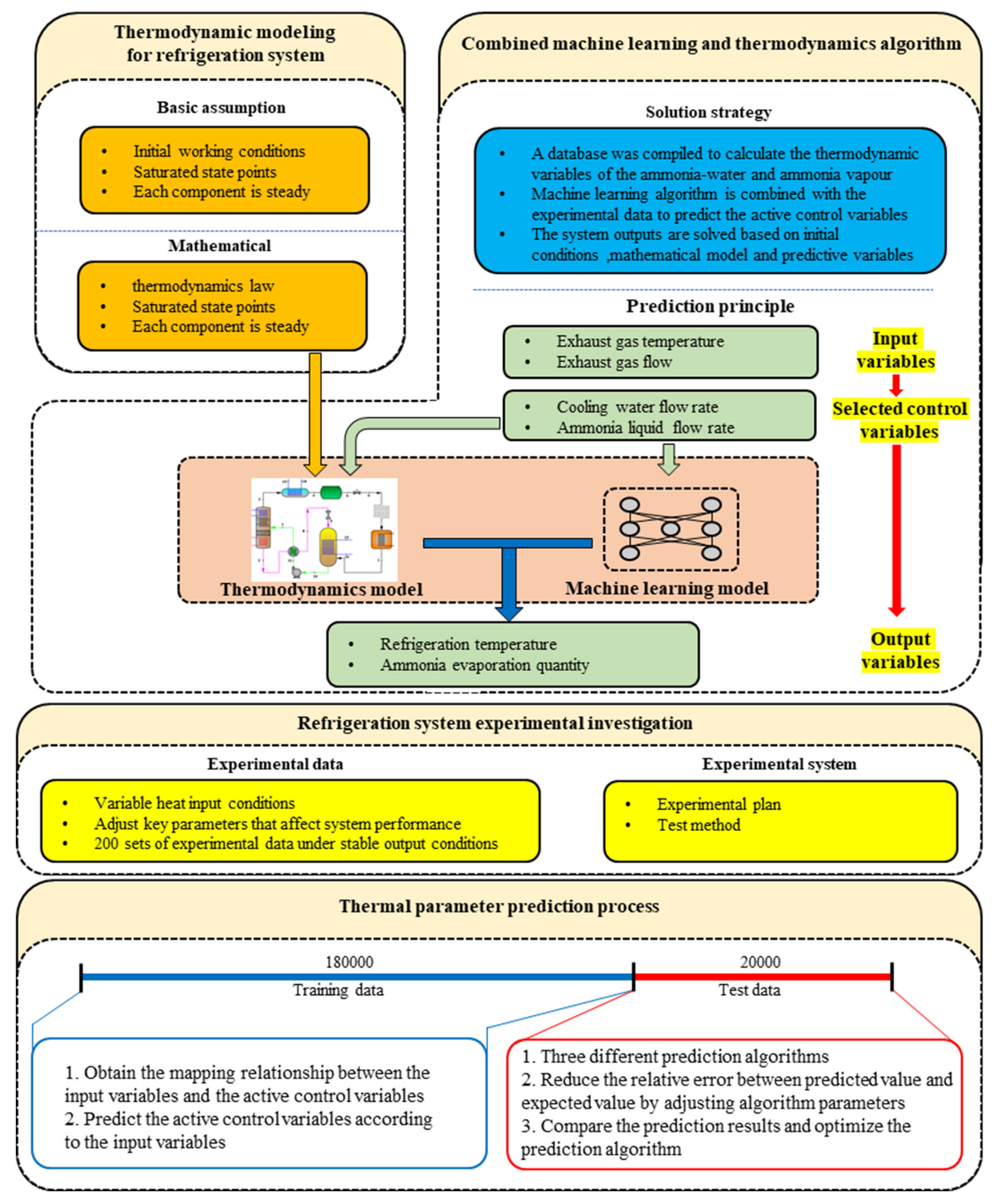
To facilitate understanding, the logical framework and main contents for parameter predictions for the absorption refrigeration system are shown in Figure 2. In the figure, the research content and interrelationships between each part are summarized. In Section 3.2 and Section 3.3, the thermodynamic analysis of the refrigeration system is carried out, including the basic assumptions and mathematical model. Based on thermodynamic analysis, the parameter prediction principle and solution strategy of the refrigeration system are provided in Section 3.4. The prediction principle covers the determination of input variables, controlled variables, and manipulated variables (prediction variables). The solution strategy includes the compilation of the database, the combination of the machine-learning algorithm and experimental data, and the calculation of system output. In Section 4, the experimental investigation of the refrigeration system is carried out, including the establishment of the experimental platform, concrete experimental plan, and record of experimental data. During the experiment, 200,000 sets of experimental data under stable output conditions were recorded. Among them, the refrigerating capacity output was basically stable at 4.85 kW, which is the expected output value of the refrigerating capacity. The experimental process and data also provide a basis for the selection of manipulated variables in Section 3.4. The main research content of Section 5 is the specific prediction process of thermodynamic parameters. The 200,000 sets of experimental data recorded in the previous section include test data and training data. The mapping relationship including input parameters and manipulated parameters is obtained through the training dataset; then, the manipulated variables can be predicted through the input variables in the test dataset. Three different prediction algorithms are introduced. The relative error between the predicted and expected values is constantly reduced by adjusting the algorithm parameters. Finally, the optimal algorithm is selected by comparing the predicted results, and system outputs such as refrigerating capacity are calculated according to the predicted values of the optimal algorithm.

3.1. Prediction Principle and Solution Strategy

The selection principle of manipulated variables is discussed as follows. Generally, an absorption refrigeration system has five degrees of freedom and the controllable variables are: expansion valve flow rate, solution pump flow rate, generator heat transfer rate, enthalpy of the working fluid of the working medium at the condenser outlet, and working fluid enthalpy at the outlet of the evaporator [47]. The expansion valve flow rate and solution pump flow rate are usually the control variables of on–off control and feedforward/feedback control. As the marine diesel engine exhaust gas heat is utilized as the source of the whole system, the heat transfer rate of the generator is determined using the exhaust temperature and exhaust gas flow rate, which cannot be controlled. Thus, in this study, the exhaust temperature and exhaust gas flow rate were designated as input variables instead of manipulated variables. The mass flow rate of cooling water and the temperature of cooling water determine the enthalpy of the ammonia working medium at the condenser outlet. During the operation, under the influence of the pump, the cooling water passes through the absorber into the condenser. A the inlet of the absorber a mass flow rate meter is installed; hence, the cooling water mass flow rate into the absorber is selected as the manipulated variable. It is significant that in the traditional control mode, the cooling water mass flow rate is hardly selected as the controllable parameter because the relationship between the working fluid enthalpy at the condenser outlet and the cooling water mass flow rate is determined using the realistic heat exchange model of the condenser, which is complex and highly inaccurate. More importantly, each actual heat exchanger has a different heat-transfer model, which causes this method to lack general applicability. The data-based machine-learning technique is independent from the heat transfer model of the condenser, which enables the cooling water mass flow rate to be selected as another manipulated variable.
Furthermore, the refrigeration capacity of the absorption system is determined using the controlled variables, and the selection principle of the controlled variables is discussed as follows. The refrigeration temperature determines the enthalpy of the working medium at the evaporator outlet. The ammonia evaporation quantity is another key variable that determines the refrigeration output. Thus, the refrigeration temperature along with the ammonia evaporation quantity can be selected as the controlled variables.
The exhaust gas temperature and exhaust gas flow rate were used as input values of the neural network, cooling water flow into the absorber and ammonia flow into the evaporator were used as control variables, and cooling temperature and ammonia evaporation were used as output values. The principle behind the procedure is based on the experimental data. In the subsequent experimental investigation, we found that the two key factors with the greatest influence on the refrigeration system performance are the flow of cooling water into the absorber and the flow of liquid ammonia into the evaporator. If these two factors are adjusted, then the refrigerating capacity output and other performance parameters can be controlled. According to the experimental and theoretical analysis results, these two factors were chosen as the manipulated variables. The mapping relationship between them and the exhaust gas conditions were also determined to predict these variables. Based on these two key factors and other initial conditions, the thermodynamic calculation and analysis of the whole system can be carried out, and the refrigerating capacity and other important output parameters of the system can be obtained.
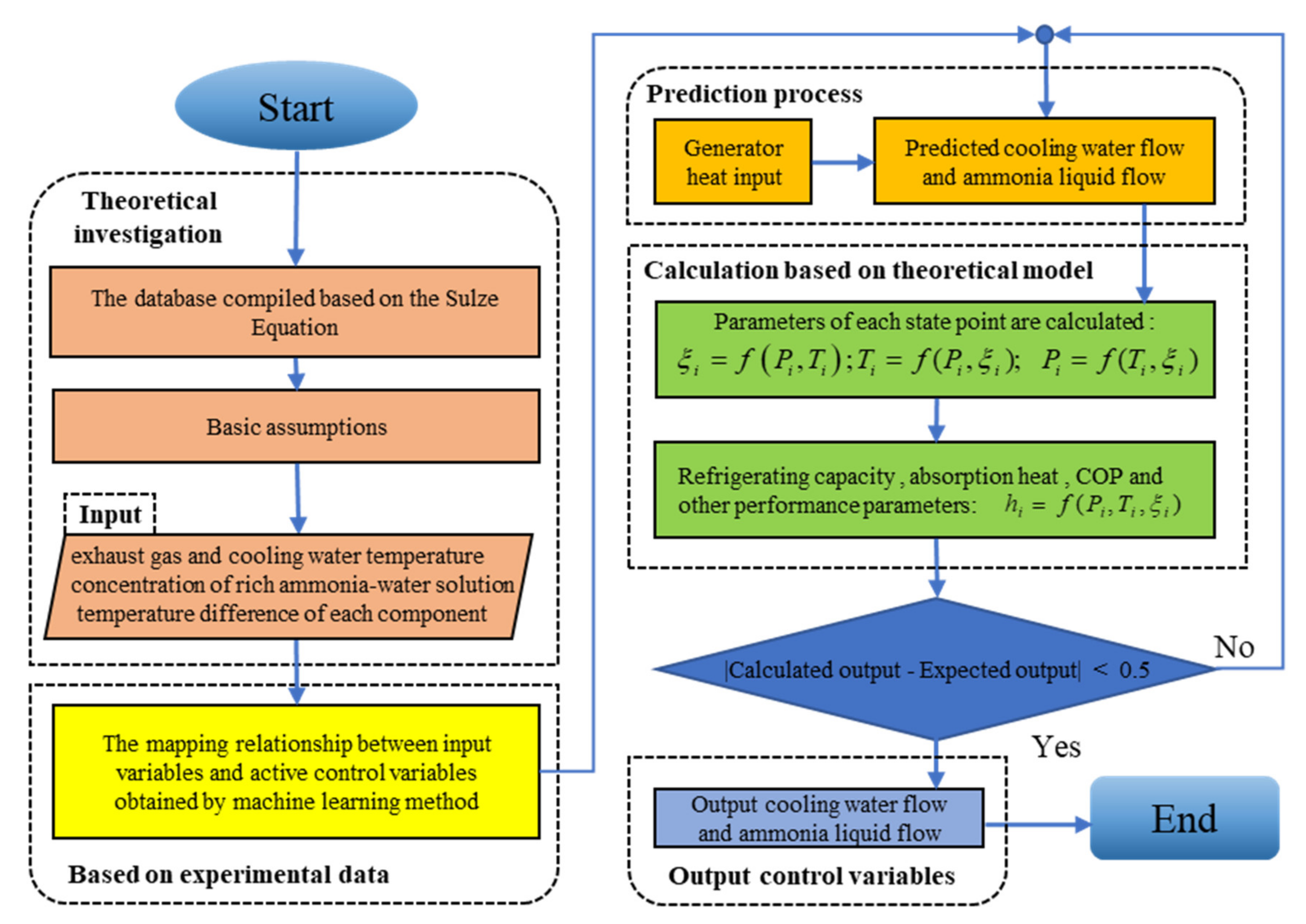
The system performance was analyzed using a program. The program which was compiled according to the Sulze equation calculated the thermodynamic variables of NH3-H2O-water and NH3 vapor [48]. Figure 3 shows the specific calculation strategy for the refrigeration system.
The process is as follows. We ran experiments and obtained experimental data. The next step was to train the data to obtain the mapping relationship between the input variables and the operation variables. On the basis of the above results, the operational variables were predicted and compared with the actual values. We substituted the predicted values of the manipulated variables into the theoretical model and compared the calculated output with the expected output. Finally, the system control parameters were adjusted according to the predicted values to realize the stable output of the cooling capacity.
In this study, the experimental setup for the NH3-H2O-based absorption refrigeration system, with exhaust gas as the heat source, was established to conduct the experiment study.

3.2. Experimental Setup

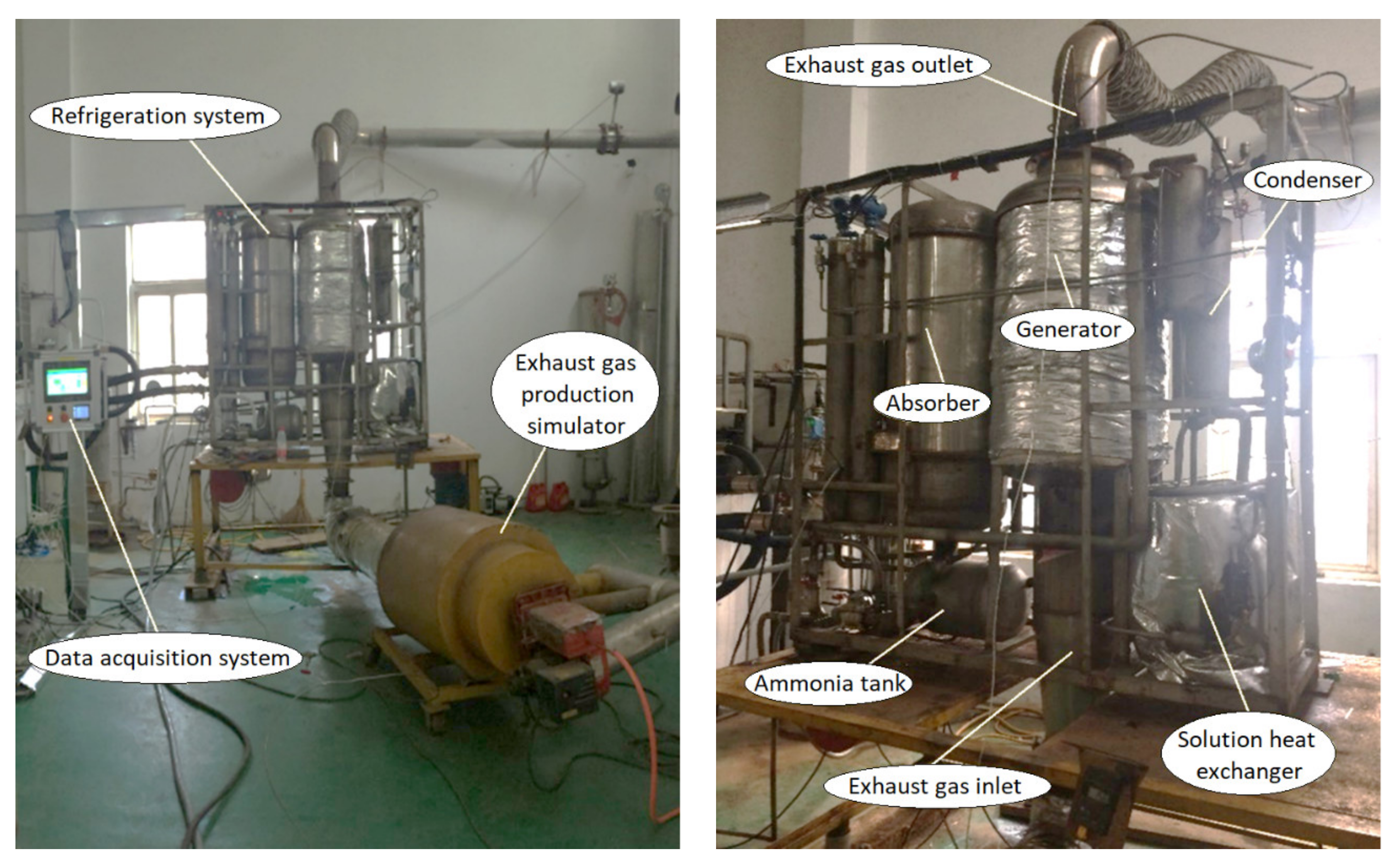
The composition of NH3-H2O-based absorption refrigeration system is shown in Figure 4. In the experiment, while the exhaust gas heat input constantly changed, the refrigerating capacity output was stabilized by adjusting the key parameters of the system. The temperature of the marine diesel exhaust gas was raised from 250 to 360 in order to test the performance. Based on the experimental process and experimental data, the flow of cooling water into the absorber and the flow of liquid ammonia into the evaporator were determined as the two most critical parameters affecting system performance. The experimental data under stable output conditions were recorded for subsequent training and prediction of the machine-learning algorithm.

3.3. Experimental Plan

The operational step is summarized as follows:
Step 1: During the experiment, the inlet exhaust gas temperature is randomly changed from 250 to 360 °C every 10 min on average.
Step 2: After the inlet exhaust gas temperature changes, the system refrigerating capacity remains stable at the same fixed value by adjusting the system control parameters, such as the flow of cooling water into the absorber, the flow of liquid ammonia into the evaporator, etc. The target refrigeration capacity is 4.85 kW, which matches the designed capacity of the experimental platform.
Step 3: After the stable operation of the whole system, the data acquisition system is used to collect and record experimental data including pressure, temperature, flow, etc. The datasets are filtered before training, and the filtering criterium is that the corresponding experimental refrigeration capacity remains between 4.75 and 4.95 kW, so that the fluctuation rate of the refrigeration capacity remains within ±2%. The datasets will be used for subsequent training and prediction processes.

3.4. Experimental Results and Analyses

The heat input of the exhaust gas can be calculated using the components and temperature at the exhaust gas inlet and outlet in the refrigeration system. The waste analyzer can measure the volume fraction of the main components in the waste gas. Nitrogen, oxygen, water, and carbon dioxide constitute 99.7% of the waste gas, so we can obtain the enthalpy of the exhaust gas. Some operating data of the refrigeration system are shown in Table 1.
In the experiment, a total of 200,000 datasets were collected. The 200,000 datasets have different exhaust gas input conditions, but the system refrigerating capacity output was kept stable at approximately 4.85 kW by adjusting the flow of cooling water into the absorber and the flow of liquid ammonia into the evaporator. The value of 4.85 kW is the expected refrigerating capacity output after the prediction and control processes. Parts of filtered dataset used for training are listed in Table 2.
In the actual prediction process, the mapping relationship between the input and manipulated variables was preliminarily obtained using the 1–180,000 sets of measured data, which were taken as training data. Next, the 180,000–200,000 sets of data were used as the test data to compare the relationship between the predicted manipulated variables and expected values. The predicted manipulated variables include the flow of cooling water into the absorber and the flow of liquid ammonia into the evaporator.

4. Combined Prediction Model Based on Machine-Learning Algorithms and Thermodynamics

In this study, a combined machine learning and thermodynamics algorithm is used to predict the controlled variables.
Three different machine-learning algorithms are shown below: backpropagation neural network (BPNN), extreme learning machine (ELM), and Elman are used to predict the controlled variables.
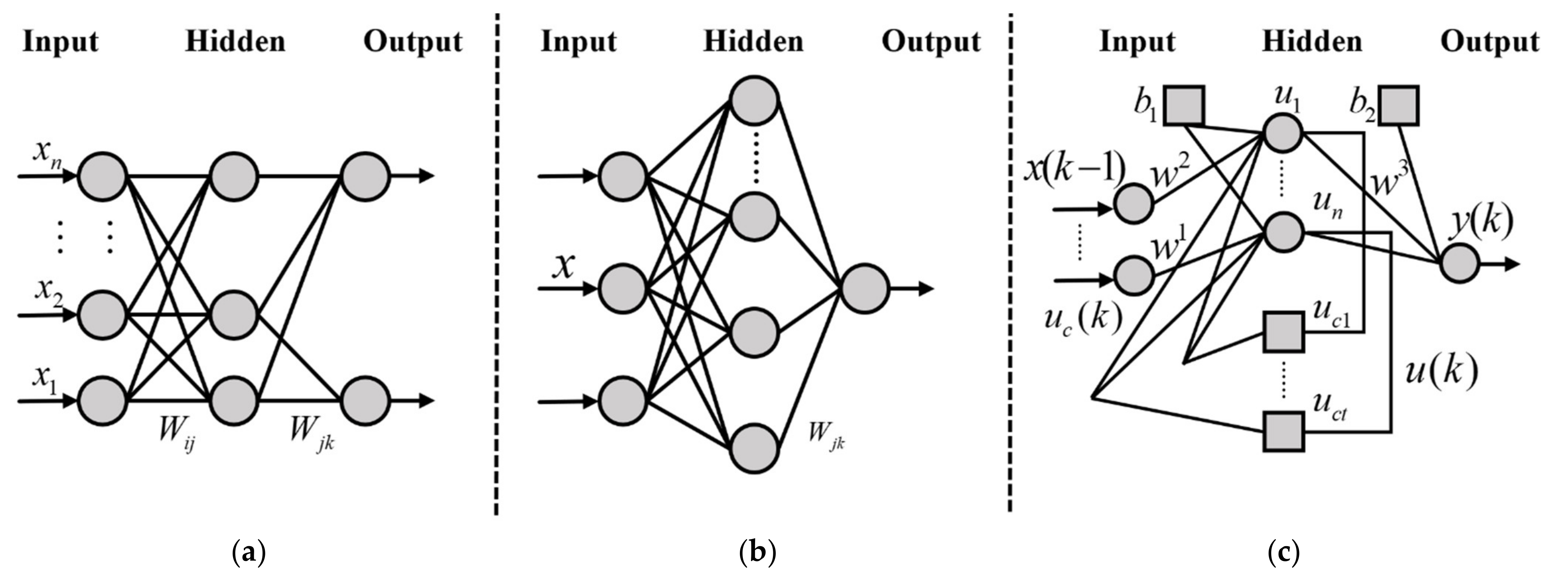
Manipulation variables are predicted and trained using three different machine-learning algorithms. The prediction process and results of the three algorithms were analyzed and compared, and the optimal algorithm was selected. The structure diagrams of the three algorithms are shown in Figure 5. The software running the algorithms is MATLAB R2016b.

4.1. BPNN Algorithm

The algorithm, characterized by forward transmission of signals and reverse propagation of error, is essentially a multi-layered feedforward neural network. The input layer, hidden layer, and output layer make up the general three-layer BPNN. The above is shown in Figure 5a.
In Figure 5a, X 1 ,   X 2 , , X n are the input values of BPNN; Y 1 , Y 2 , , Y m are the predicted values; and w i j , w j k are the weight values. In Figure 5a, the We equivalent BPNN to a nonlinear function can be seen. The input values are independent variables and the predicted values are dependent variables. When the input vector has the dimension N, the output vector has the dimension M. The processing flow of BPNN can be regarded as the mapping of N-dimensional vectors to M-dimensional vectors.
Before prediction, the BPNN needs a lot of data for training to improve the accuracy of prediction. BPNN-specific prediction steps are as follows:
Step 1: Initialize the network according to the input and output sequences ( X , Y ) of the system and determine the input layer dimension n , hidden layer dimension l , and output layer dimension m . The connection weights of neurons in the input layer, hidden layer, and output layer, w i j and w j k , are initialized. The thresholds of neurons in hidden layer a and output layer b are initialized, and the learning rate η and neuron excitation function f are provided.
Step 2: Compute the output of the hidden layer. The initialized input variable X , the connection weight w i j between the input layer and the hidden layer, and the hidden layer threshold a are used to calculate the hidden layer output H .
H j = f ( i = 1 n w i j x i a j )      j = 1 , 2 , , l
Step 3: Calculate the output layer output. The connection weight w j k , the output of the hidden layer H , and the threshold b calculate the predictive output O .
O k = j = 1 l H j w j k   b k     k = 1 , 2 , , m
Step 4: Calculate the error. The expected output Y and the predicted output O compute the prediction error e .
e k   = Y k O k     k = 1 , 2 , , m
Step 5: Update the weights. Prediction error e updates connection weights w i j and w j k .
w i j = w i j + η H j ( 1 H j ) x ( i ) k = 1 m w j k e k     i = 1 , 2 , , n ;    j = 1 , 2 , , l
w j k = w j k + η H j e k     j = 1 , 2 , , l ;    k = 1 , 2 , , m
Step 6: The threshold is updated. The prediction error e updates node thresholds a and b .
a j = a j + η H j ( 1 H j ) k = 1 m w j k e k     j = 1 , 2 , , l
b k = b k + e k     k = 1 , 2 , , m
Step 7: Check the completion of the algorithm iteration. If not finished, return to Step 2.
Two manipulated variables: the cooling water flow into the absorber, and liquid ammonia flow into the evaporator, will be predicted by the trained BPNN algorithm.

4.2. ELM Algorithm

The ELM algorithm structure diagram is shown in Figure 5b. Assuming that the number of input layer neurons is d , the number of hidden layer neurons is l , and the activation function between input layer and hidden layer is f , the sample datasets are { X i , y i } i = 1 n , and X i = [ x i 1 , x i 2 , , x i d ] T R d , where n is the total number of sample datasets. W j is the weight vector between the j th hidden layer neurons and input vector X i . b j is the threshold of the j th hidden layer neurons. θ j is the weight between the j th hidden layer neurons and output layer nodes and o i is the output of the i th sample. Then, the mathematical relationship between input and output is
j = 1 l f j ( W j , b j , X i ) θ j = o i ,    i = 1 , 2 , , n ;    j = 1 , 2 , , l
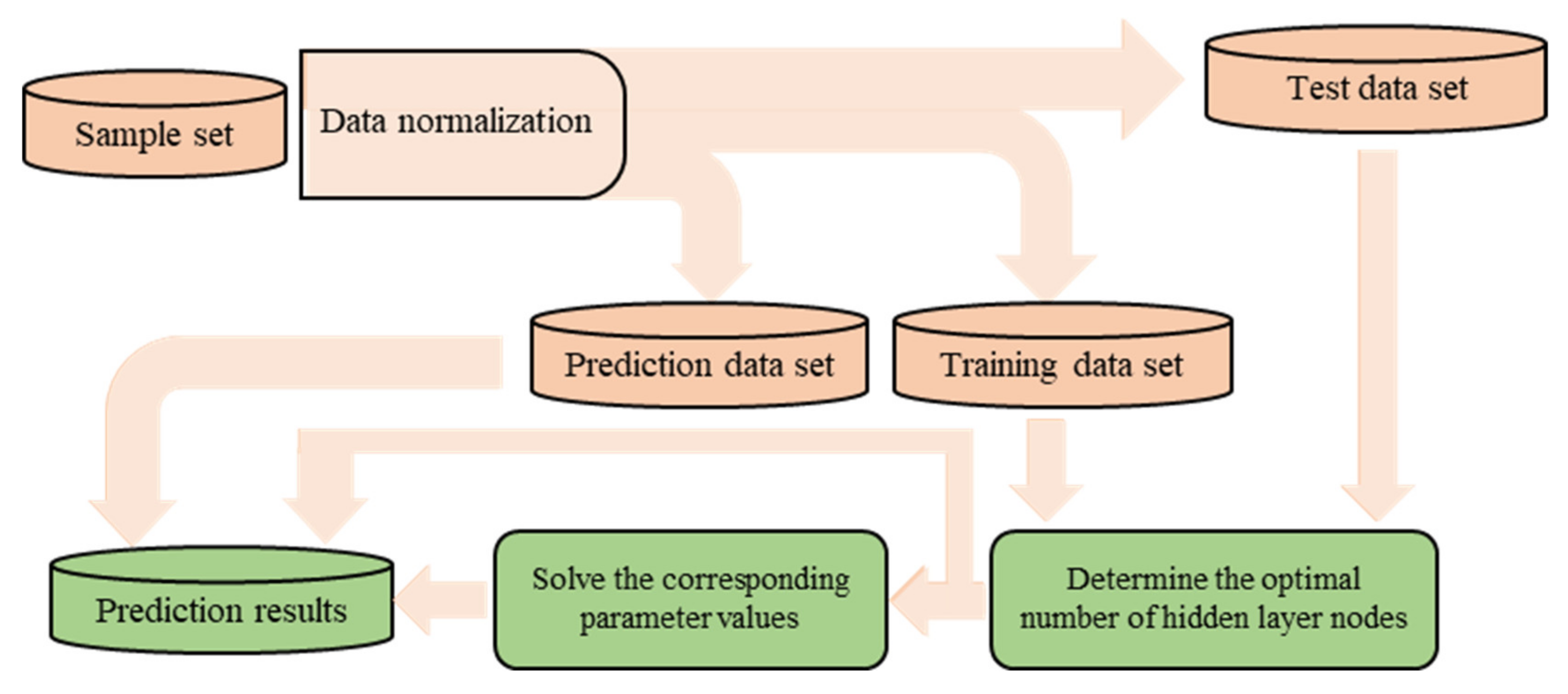
In the ELM prediction process, the sample consists of a test set, training set, and prediction set. All input data should be normalized. Then, the optimal number of hidden layer nodes is determined and the corresponding θ is solved. Finally, according to the above operations, the optimal parameters are obtained and applied to the prediction data set. A schematic of the ELM algorithm prediction procedure is shown in Figure 6.
Two manipulated variables, the cooling water flow into the absorber and liquid ammonia flow into the evaporator, will be predicted by the trained ELM algorithm.

4.3. Elman Algorithm

The Elman algorithm, proposed by Elman, is a feedforward neural network algorithm.
As shown in Figure 5c, the Elman algorithm consists of four parts: the input layer, hidden layer, receive layer, and output layer. The relationships between the hidden layer, input layer, and output layer are consistent with that of the feedforward network. The input layer neurons play the role of signal transmission, while the hidden layer neurons take linear or non-linear functions as the transfer function. The receiving layer neurons are used to remember the output value of the hidden layer neurons in the previous moment and return it to the network’s input; the output layer neurons play the role of linear weighting.
The non-linear state space expressions of the Elman algorithm are as follows:
y ( k ) = g ( w 3 u ( k ) )
u ( k ) = f ( w 1 u c ( k ) + w 2 ( x ( k 1 ) ) )
u c ( k ) = u ( k 1 )
where y is the output node vector, u is the unit vector of the middle layer node, x is the input vector, u c is the feedback state vector, w 3 is the connection weight between the middle layer and the output layer, w 2 is the connection weight between the input layer and the middle layer, w 1 is the connection weight between the receiving layer and the middle layer, g is the transfer function of the output layer neuron, and f is the transfer function of the middle layer neurons.
The Elman algorithm mainly adjusts the number of hidden layer neurons to obtain a unique global optimal solution during the process of adjusting hyperparameters.

4.4. Thermodynamic Model

The performance of the refrigeration system is analyzed using thermodynamics. The mathematical model is established and the program used to solve the equation is programmed. The prediction principle and solution strategy of refrigeration system Are introduced in detail. Basic assumptions.
The following assumptions were made for system modeling:
(1)
The initial concentration of rich ammonia–water solution is available.
(2)
The inlet temperature of cooling water is available.
(3)
The NH3-H2O solution and vapor reaches saturation at the output end of the absorber and reflux condenser.
(4)
The components of the refrigeration system are in a steady state.
(5)
All heat exchangers can meet the minimum heat-transfer requirements.

4.5. Mathematical Model for Absorption Refrigeration Cycle

The absorption refrigeration system is analyzed and its performance is evaluated. A mathematical model of the system is proposed based on the first law of thermodynamics. The equations are as follows:
Δ o u t i n m i = 0
Δ o u t i n ξ i · m i = 0
Q G / E = Δ o u t i n m i · h i
Q C / A = Δ i n o u t m i · h i
Q D = U D A D Δ T D
1 U D = A o A i n h o + A o h w + 1 h i n + δ
COP = Q E / Q G
where m i is the mass flow rate of the working fluid, ξ i is the ammonia concentration, and h i is the enthalpy of the working fluid at each state point in the absorption refrigeration system. Q G is the generation heat input and Q E is the refrigerating capacity output. Q C / A is the condensation/absorption heat output. Q D is the heat exchange of the components, U D denotes the overall heat transfer coefficient of the components, A D is the heat exchange area of the components, and Δ T D is the log mean temperature difference of the components. A o and A i n are the external and internal heat exchange areas. h o and h i n are the heat transfer coefficients of the outer side (heating/cooling side) and the heat transfer coefficients of the inner side (working medium side), respectively, and h w is the conductivity of the heat-transfer wall. δ is fouling factor of the heat exchange surface. The system coefficient of performance (COP) was used to evaluate system performance.
The accuracy of the theoretical model mentioned above was verified by the experimental results. With regard to the selection of theoretical model parameters, please refer to [35].

4.6. Comparison and Optimization of Prediction Algorithms

Two manipulated variables, the cooling water flow into the absorber and liquid ammonia flow into the evaporator, were predicted by the trained BPNN algorithm, ELM algorithm, and Elman algorithm. The predicted results and analyses are as follows.
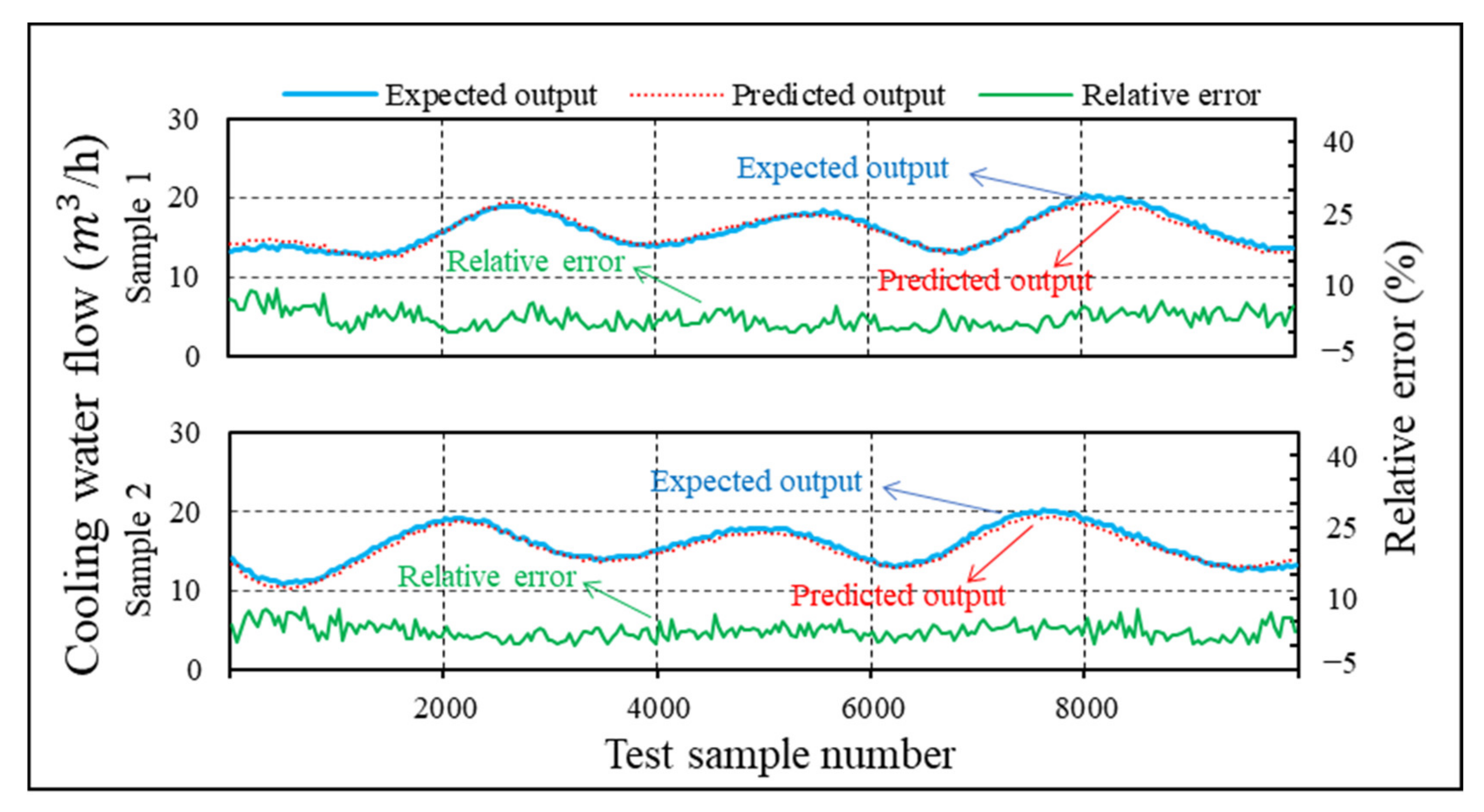
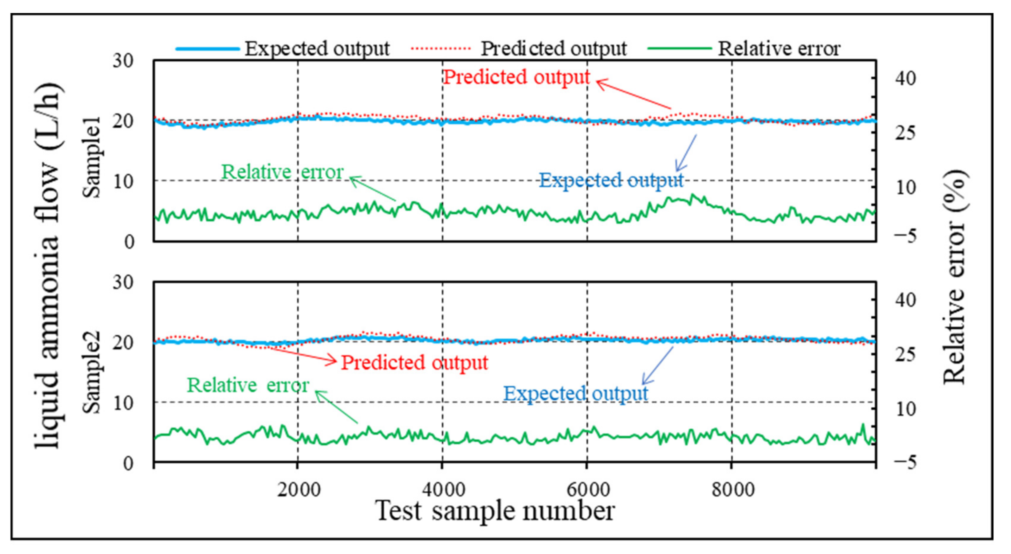
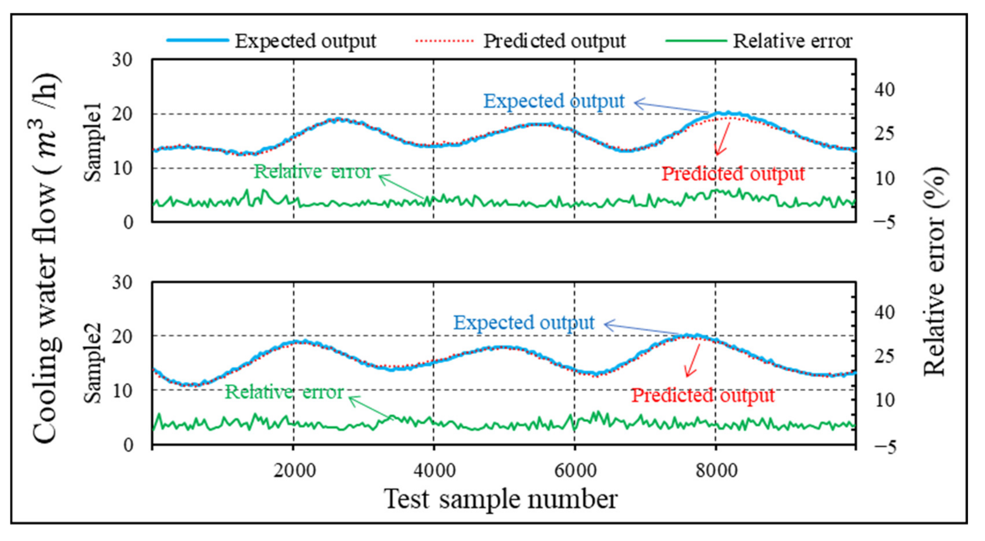
Figure 7 and Figure 8 show the comparison between the BPNN-predicted results and expected values for two manipulated variables. The predicted values agree with the expected values. The maximum relative error between the predicted cooling water flow and the expected value is approximately 5.8%. The maximum relative error between the predicted liquid ammonia flow and expected value is approximately 7.2%.
Figure 9 and Figure 10 show the comparison between the ELM-predicted results and the expected values for two manipulated variables. The predicted values are very close to the expected values and the prediction result of cooling water flow is relatively good. The maximum relative error between the predicted cooling water flow and expected value is approximately 2.5%. The maximum relative error between the predicted liquid ammonia flow and expected value is approximately 5.1%.
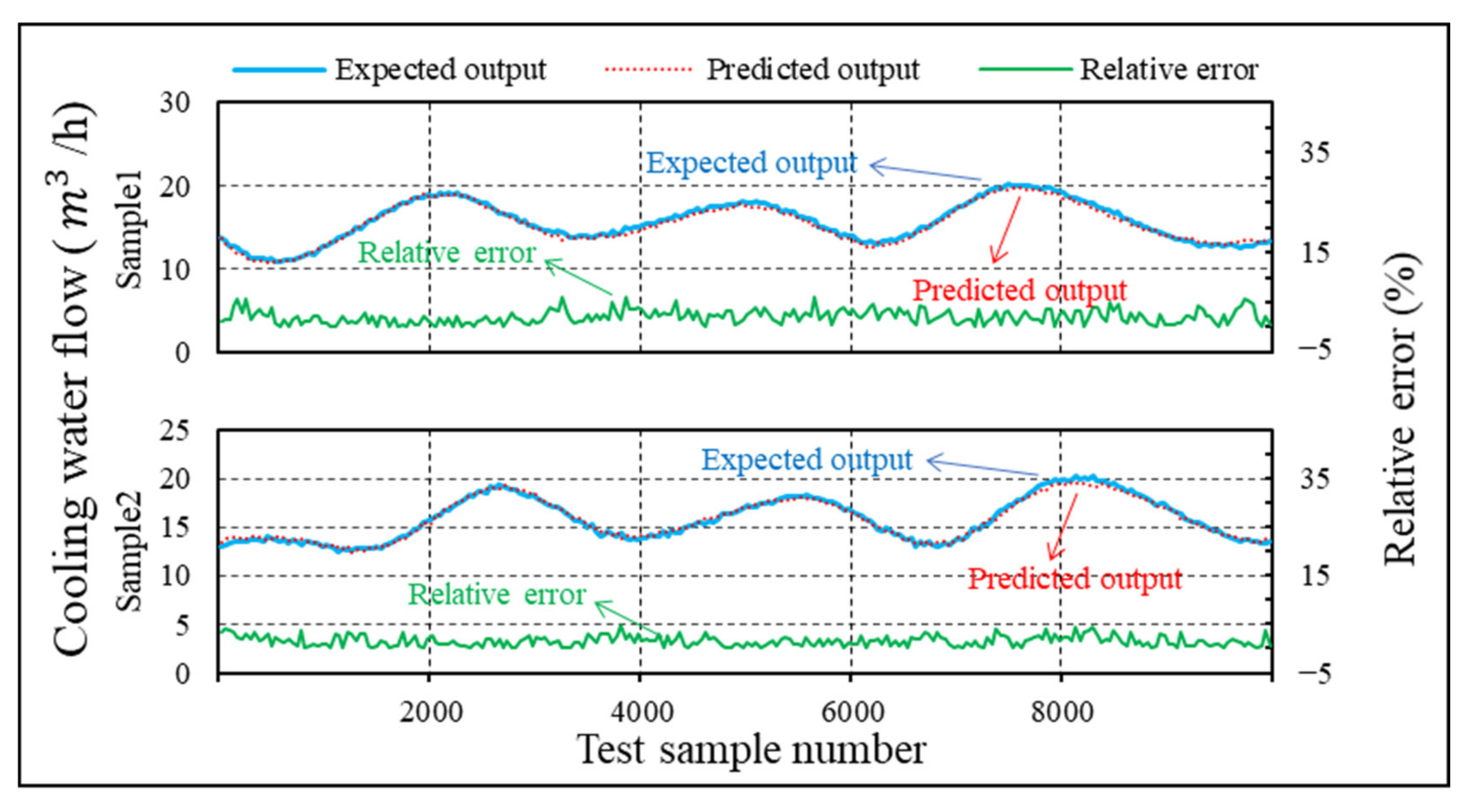
Figure 11 and Figure 12 show the comparison between the Elman-predicted results and expected values for two manipulated variables. The changing trends of the predicted and expected values are basically identical. The prediction result of cooling water flow is relatively good. The maximum relative error between the predicted cooling water flow and expected value is approximately 4.1%. The maximum relative error between the predicted liquid ammonia flow and expected value is approximately 5.6%.
The results of the three different prediction algorithms for two manipulated variables are shown in Table 3. It can be seen that the maximum relative errors between the predicted and expected values of the two manipulated variables have little difference. Therefore, the total error sum of 20 test dataset samples predicted by the ELM algorithm is relatively small. Moreover, the ELM algorithm has a fast learning speed and good generalization performance. Therefore, the ELM algorithm was selected as the final optimal prediction algorithm.

4.7. System Performance Based on the Predicted Value of the Optimization Algorithm

In this section, the predictive control variables obtained by the optimization algorithm are substituted into the theoretical model mentioned above. Then, the system refrigerating capacity is calculated in combination with other initial conditions. The calculated refrigerating capacity is compared with the expected value to determine whether the stability control can be achieved. We reiterate that the theoretical model was verified by experimental investigation. To illustrate the accuracy of the model, specific data are provided for the example in Table 4.
As shown in the table, relative error between the theoretical and experimental refrigeration output is less than 5%. Therefore, the theoretical model has high reliability and can be used to test the actual refrigerating capacity control value.
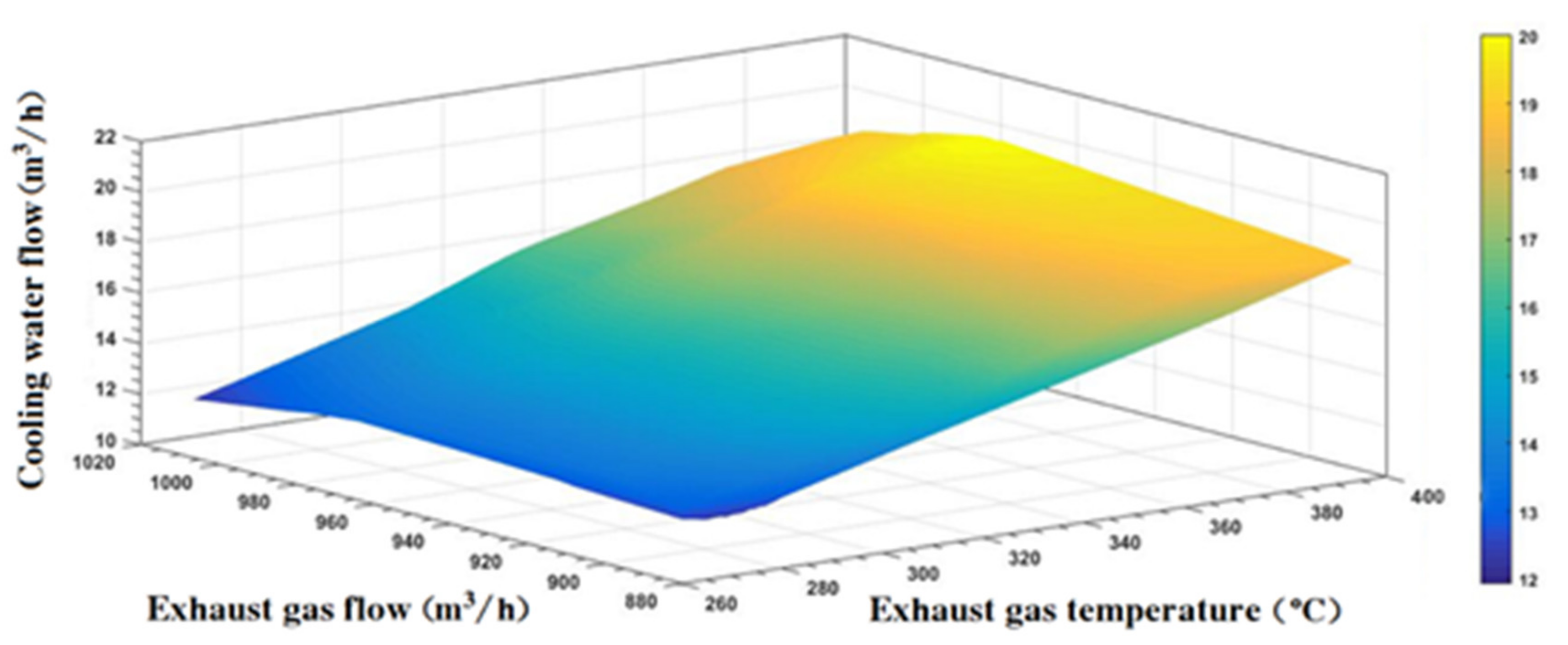
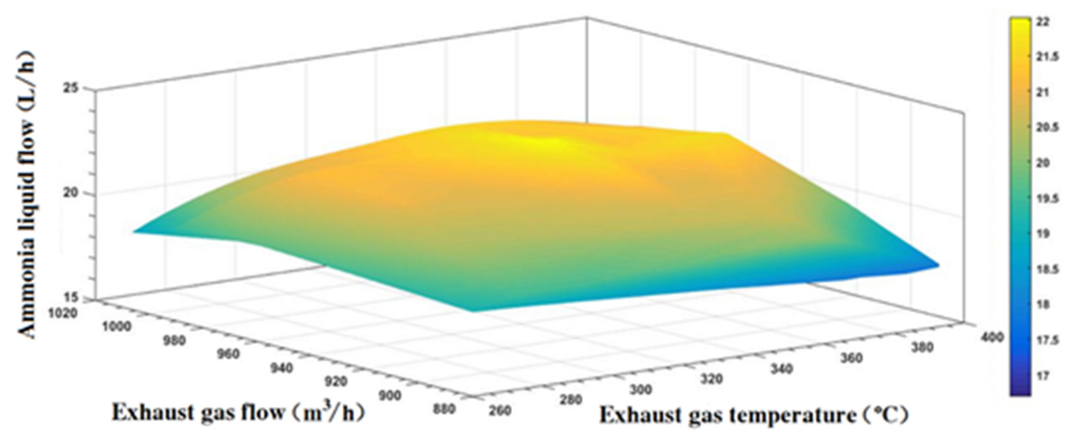
The corresponding relationships between the prediction results of two manipulated variables using the optimal ELM algorithm and the input parameters of heat source exhaust gas are shown in Figure 13 and Figure 14.
Figure 13 shows the corresponding relationship between the predicted cooling water flow and input parameters of the heat source exhaust gas. The exhaust gas temperature is the main factor affecting the input heat of the system. The system heat input increases with increasing exhaust gas temperature. Therefore, the predicted cooling water flow of the system is also increased to maintain the stability of the refrigerating capacity output.
Figure 14 shows the corresponding relationship between the predicted liquid ammonia flow and input parameters of the heat source exhaust gas. The liquid ammonia flow into the evaporator is the main factor affecting the refrigerating capacity output. As can be seen from the figure, when the stable refrigerating capacity output of the system is taken as the control objective, the predicted liquid ammonia flow is maintained within the range of 20 ± 2 L/h and is relatively stable under the condition of changing heat input.
According to the solution strategy, an analysis of the thermodynamic parameters of the refrigeration system was carried out based on the ELM-predicted cooling water flow and liquid ammonia flow. The calculated refrigerating capacity output is shown in Figure 15.
Figure 15 shows the relationship between system refrigerating capacity output and predicted cooling water flow and liquid ammonia flow. It can be seen that under the predicted cooling water flow and liquid ammonia flow conditions, the refrigerating capacity output obtained by thermodynamic calculation is basically stable within the range 4.8–5.2 kW. The maximum relative error with the expected refrigerating capacity output value of 4.85 kW is 7.2%, which can be considered as reaching the expected control target of a stable refrigerating capacity output.

5. Conclusions

In order to solve the problem that the cooling output of ammonia absorption refrigeration systems fluctuates greatly due to the unstable exhaust energy of a diesel engine under fluctuating operating conditions, an active control method based on the machine-learning algorithm was proposed. This method combines machine-learning and thermodynamic models, making the machine-learning method effectively combine with the real physical scenes behind it. It was successfully applied for the control of an exhaust heat refrigeration system. The mathematical model based on the law of thermodynamics and the solving process to predict its performance were established. A prototype of the system was established and several experiments were carried out. During the experiment, the system refrigerating capacity output was maintained at nearly 4.85 kW by adjusting the key parameters as the inlet exhaust gas temperature increased from 250 to 360 °C. Data on the whole system under stable output conditions were recorded for training and prediction of the machine-learning algorithm. Three different machine-learning algorithms were used to predict the key control parameters. By comparing the prediction results of the three algorithms, the optimal prediction algorithm was selected. The system cooling capacity was calculated according to the predicted system control parameters. According to the above experiments and analysis, the following conclusions can be drawn.
  • The two most critical parameters affecting the system refrigeration performance, i.e., the cooling water flow into the absorber and liquid ammonia flow into the evaporator, were determined based on the experimental process and experimental data and were selected as the two manipulated variables.
  • The BPNN algorithm results show that the maximum relative error between the predicted cooling water flow and expected value is approximately 5.8%. The maximum relative error between the predicted liquid ammonia flow and expected value is approximately 7.2%. The ELM algorithm results show that the maximum relative error between the predicted cooling water flow and expected value is approximately 2.5%. The maximum relative error between the predicted liquid ammonia flow and expected value is approximately 5.1%. The Elman algorithm results show that the maximum relative error between the predicted cooling water flow and expected value is approximately 4.1%. The maximum relative error between the predicted liquid ammonia flow and the expected value is approximately 5.6%.
  • The ELM algorithm was selected as the final optimal prediction algorithm owing to its relatively fast learning speed, good generalization performance, and small error sum of the test set.
  • The calculated refrigerating capacity output based on the ELM algorithm prediction ranged from 4.8 to 5.2 kW. The maximum relative error with the expected refrigerating capacity output of 4.85 kW was 7.2%.
  • There is a certain coupling relationship between the exhaust heat of a marine diesel engine and the absorption refrigeration system. Application scenarios of absorption refrigeration systems, such as indoor refrigeration and cold-storage refrigeration, will also affect the performance of the refrigeration system. In addition, the aging of mechanical systems and sensors can affect the prediction accuracy, so online learning can be used to enhance the performance.

Author Contributions

Conceptualization, Y.S. and P.S.; methodology, Y.S.; software, Y.S. and P.S.; validation, Z.Z. and S.Z.; data curation, Z.Z. and J.Z.; writing—original draft preparation, Y.S. and P.S.; writing—review and editing, P.S.; supervision, N.M. and J.Z.; project administration, N.M. and J.Z.; funding acquisition, N.M. All authors have read and agreed to the published version of the manuscript.

Funding

This work was financially supported by the Youth Innovation in Science and Technology Support Project of Shandong College and University (2019KJB013) and Natural Science Foundation of Shandong Province (ZR2020ME186).

Data Availability Statement

Not applicable.

Conflicts of Interest

The authors declare no conflict of interest.

Nomenclature

Symbols Greek symbols
ACross-sectional area, m2ηLearn rate, %
XSets of input values for the networkθWeight between hidden layer neurons
YSets of output values for the networkξAmmonia concentration
M, NDimension numberδFouling factor of the heat exchange surface
a, bNode thresholdsSubscript
OPredictive output1, 2, 3 … State points
ePrediction errora, b, cCross section
dNumber of input layer neuronsucFeedback state vector
lNumber of hidden layer neuronsw3Connection weight between the middle layer and output layer
fActivation function between the input layer and hidden layerw2Connection weight between the input layer and middle layer
nTotal number of samplesw1Connection weight between the receiving layer and middle layer
wWeight valuesmiMass flow rate of the working fluid, L/min
HHidden layerQGGeneration heat input, Kj
yOutput node vectorQERefrigerating capacity output
uUnit vector of middle layer nodeQC/ACondensation/absorption heat output
xInput vectorQDHeat exchange of the components
gTransfer function of the output layer neuronUDThe overall heat transfer coefficient of the components
hEnthalpy of the working fluidADHeat exchange area of the components
Acronyms TDLog mean temperature difference of the components
ORCOrganic Rankine CycleAoExternal heat exchange areas, m3
ELMExtreme learning machineAinInternal heat exchange areas, m3
BPNNBack propagation neural networkhoHeat transfer coefficients of the outer side (heating/cooling side)
COPCoefficient of performancehinThe heat transfer coefficients of the inner side (working medium side)
MEDMulti-effect distillationhwThe conductivity of the heat transfer wall
MLAMachine-learning algorithms

References

  1. Hossain, F.M.; Nabi, N.; Brown, R.J. Investigation of diesel engine performance and exhaust emissions of microalgae fuel components in a turbocharged diesel engine. Energy Convers. Manag. 2019, 186, 220–228. [Google Scholar] [CrossRef]
  2. Nour, M.; Attia, A.M.; Nada, S.A. Combustion, performance and emission analysis of diesel engine fuelled by higher alcohols (butanol, octanol and heptanol)/diesel blends. Energy Convers. Manag. 2019, 185, 313–329. [Google Scholar] [CrossRef]
  3. Petranović, Z.; Sjerić, M.; Taritaš, I.; Vujanović, M.; Kozarac, D. Study of advanced engine operating strategies on a turbocharged diesel engine by using coupled numerical approaches. Energy Convers. Manag. 2018, 171, 1–11. [Google Scholar] [CrossRef]
  4. Leng, L.; Shi, L.; Gui, Y.; Liu, B.; Deng, K. Research Progress on Intelligent Control Technology of Marine Diesel Engine. J. Propuls. Technol. 2021, 42, 1186–1194. [Google Scholar]
  5. Fu, J.; Liu, J.; Feng, R.; Yang, Y.; Wang, L.; Wang, Y. Energy and exergy analysis on gasoline engine based on mapping characteristics experiment. Appl. Energy 2013, 102, 622–630. [Google Scholar] [CrossRef]
  6. Wang, X.; Sun, B.-G.; Luo, Q.-H. Energy and exergy analysis of a turbocharged hydrogen internal combustion engine. Int. J. Hydrog. Energy 2018, 44, 5551–5563. [Google Scholar] [CrossRef]
  7. Kiani, M.K.D.; Rostami, S.; Eslami, M.; Yusaf, T.; Sendilvelan, S. The effect of inlet temperature and spark timing on thermo-mechanical, chemical and the total exergy of an SI engine using bioethanol-gasoline blends. Energy Convers. Manag. 2018, 165, 344–353. [Google Scholar] [CrossRef]
  8. Patel, K.R.; Dhiman, V.D. A review on emission and performance of water diesel micro-emulsified mixture-diesel engine. Int. J. Environ. Sci. Technol. 2021, 19, 8027–8042. [Google Scholar] [CrossRef]
  9. Di Blasio, G.; Belgiorno, G.; Beatrice, C. Effects on performances, emissions and particle size distributions of a dual fuel (methane-diesel) light-duty engine varying the compression ratio. Appl. Energy 2017, 204, 726–740. [Google Scholar] [CrossRef]
  10. Verhelst, S.; Turner, J.W.; Sileghem, L.; Vancoillie, J. Methanol as a fuel for internal combustion engines. Prog. Energy Combust. Sci. 2018, 70, 43–88. [Google Scholar] [CrossRef]
  11. Fontana, G.; Galloni, E.; Ianniello, R.; Lanni, D.; Beatrice, C.; Di Biasio, G. Numerical analyses of spray development and combustion process with diesel-gasoline-ethanol mixtures in compression-ignition engines. In Proceedings of the Second International Conference on Material Science, Smart Structures and Applications: ICMSS-2019, Erode, India, 21–22 November 2019. [Google Scholar] [CrossRef]
  12. Kyriakidis, F.; Sørensen, K.; Singh, S.; Condra, T. Modeling and optimization of integrated exhaust gas recirculation and multi-stage waste heat recovery in marine engines. Energy Convers. Manag. 2017, 151, 286–295. [Google Scholar] [CrossRef]
  13. Kim, S.; Choi, K.; Lee, K.; Kim, K. Evaluation of automotive waste heat recovery for various driving modes. Energy 2016, 106, 579–589. [Google Scholar] [CrossRef]
  14. Fu, J.; Liu, J.; Wang, Y.; Deng, B.; Yang, Y.; Feng, R.; Yang, J. A comparative study on various turbocharging approaches based on IC engine exhaust gas energy recovery. Appl. Energy 2014, 113, 248–257. [Google Scholar] [CrossRef]
  15. Vale, S.; Heber, L.; Coelho, P.; Silva, C. Parametric study of a thermoelectric generator system for exhaust gas energy recovery in diesel road freight transportation. Energy Convers. Manag. 2016, 133, 167–177. [Google Scholar] [CrossRef]
  16. Hoang, A.T. Waste heat recovery from diesel engines based on Organic Rankine Cycle. Appl. Energy 2018, 231, 138–166. [Google Scholar] [CrossRef]
  17. Wang, D.; Li, Y.; Li, D.; Xia, Y.; Zhang, J. A review on adsorption refrigeration technology and adsorption deterioration in physical adsorption systems. Renew. Sustain. Energy Rev. 2010, 14, 344–353. [Google Scholar] [CrossRef]
  18. Salek, F.; Moghaddam, A.N.; Naserian, M.M. Thermodynamic analysis of diesel engine coupled with ORC and absorption refrigeration cycle. Energy Convers. Manag. 2017, 140, 240–246. [Google Scholar] [CrossRef]
  19. Fu, J.; Liu, J.; Deng, B.; Feng, R.; Yang, J.; Zhou, F.; Zhao, X. An approach for exhaust gas energy recovery of internal combustion engine: Steam-assisted turbocharging. Energy Convers. Manag. 2014, 85, 234–244. [Google Scholar] [CrossRef]
  20. Mostafavi, S.A.; Mahmoudi, M. Modeling and fabricating a prototype of a thermoelectric generator system of heat energy recovery from hot exhaust gases and evaluating the effects of important system parameters. Appl. Therm. Eng. 2018, 132, 624–636. [Google Scholar] [CrossRef]
  21. Mohamed, E.S. Development and performance analysis of a TEG system using exhaust recovery for a light diesel vehicle with assessment of fuel economy and emissions. Appl. Therm. Eng. 2018, 147, 661–674. [Google Scholar] [CrossRef]
  22. Jiménez-Arreola, M.; Wieland, C.; Romagnoli, A. Direct vs indirect evaporation in Organic Rankine Cycle (ORC) systems: A comparison of the dynamic behavior for waste heat recovery of engine exhaust. Appl. Energy 2019, 242, 439–452. [Google Scholar] [CrossRef]
  23. Mohammadkhani, F.; Yari, M. A 0D model for diesel engine simulation and employing a transcritical dual loop Organic Rankine Cycle (ORC) for waste heat recovery from its exhaust and coolant: Thermodynamic and economic analysis. Appl. Therm. Eng. 2019, 150, 329–347. [Google Scholar] [CrossRef]
  24. Goyal, P.; Baredar, P.; Mittal, A.; Siddiqui, A.R. Adsorption refrigeration technology—An overview of theory and its solar energy applications. Renew. Sustain. Energy Rev. 2016, 53, 1389–1410. [Google Scholar] [CrossRef]
  25. Wang, R.; Xia, Z.; Wang, L.; Lu, Z.; Li, S.; Li, T.; Wu, J.; He, S. Heat transfer design in adsorption refrigeration systems for efficient use of low-grade thermal energy. Energy 2011, 36, 5425–5439. [Google Scholar] [CrossRef]
  26. Li, Y.; Wang, L.; Yuan, Z.; Chen, Q. Enhancement of heat transfer in adsorption bed of vacuum-tube with fins. Appl. Therm. Eng. 2019, 153, 291–298. [Google Scholar] [CrossRef]
  27. Cui, P.; Yu, M.; Liu, Z.; Zhu, Z.; Yang, S. Energy, exergy, and economic (3E) analyses and multi-objective optimization of a cascade absorption refrigeration system for low-grade waste heat recovery. Energy Convers. Manag. 2019, 184, 249–261. [Google Scholar] [CrossRef]
  28. Salmi, W.; Vanttola, J.; Elg, M.; Kuosa, M.; Lahdelma, R. Using waste heat of ship as energy source for an absorption refrigeration system. Appl. Therm. Eng. 2017, 115, 501–516. [Google Scholar] [CrossRef]
  29. She, X.; Yin, Y.; Xu, M.; Zhang, X. A novel low-grade heat-driven absorption refrigeration system with LiCl–H2O and LiBr–H2O working pairs. Int. J. Refrig. 2015, 58, 219–234. [Google Scholar] [CrossRef]
  30. Maryami, R.; Dehghan, A. An exergy based comparative study between LiBr/water absorption refrigeration systems from half effect to triple effect. Appl. Therm. Eng. 2017, 124, 103–123. [Google Scholar] [CrossRef]
  31. Cerezo, J.; Bourouis, M.; Vallès, M.; Coronas, A.; Best, R. Experimental study of an ammonia–water bubble absorber using a plate heat exchanger for absorption refrigeration machines. Appl. Therm. Eng. 2009, 29, 1005–1011. [Google Scholar] [CrossRef] [Green Version]
  32. Ibrahim, N.I.; Al-Sulaiman, F.A.; Ani, F.N. Performance characteristics of a solar driven lithium bromide-water absorption chiller integrated with absorption energy storage. Energy Convers. Manag. 2017, 150, 188–200. [Google Scholar] [CrossRef]
  33. Alelyani, S.M.; Fette, N.W.; Stechel, E.B.; Doron, P.; Phelan, P.E. Techno-economic analysis of combined ammonia-water absorption refrigeration and desalination. Energy Convers. Manag. 2017, 143, 493–504. [Google Scholar] [CrossRef]
  34. Srikhirin, P.; Aphornratana, S.; Chungpaibulpatana, S. A review of absorption refrigeration technologies. Renew. Sustain. Energy Rev. 2001, 5, 343–372. [Google Scholar] [CrossRef]
  35. Li, Y.; Hu, R. Exergy-analysis based comparative study of absorption refrigeration and electric compression refrigeration in CCHP systems. Appl. Therm. Eng. 2016, 93, 1228–1237. [Google Scholar] [CrossRef]
  36. Xinxing, Z.; Guozhen, X.; Fanying, K. Study on the Relationship between the Frequency Conversion Control and Stability of Lithium Bromide Absorption Chiller System. J. Beijing Univ. Civ. Eng. Archit. 2009, 8, 37–40. [Google Scholar]
  37. Yuan, H.; Sun, P.; Zhang, J.; Sun, K.; Mei, N.; Zhou, P. Theoretical and experimental investigation of an absorption refrigeration and pre-desalination system for marine engine exhaust gas heat recovery. Appl. Therm. Eng. 2019, 150, 224–236. [Google Scholar] [CrossRef]
  38. Machado, D.O.; Sánchez, A.J.; Gallego, A.J.; de Andrade, G.A.; Normey-Rico, J.E.; Bordons, C.; Camacho, E.F. Split-range control for improved operation of solar absorption cooling plants. Renew. Energy 2022, 192, 361–372. [Google Scholar] [CrossRef]
  39. Kim, B.; Park, J. Dynamic simulation of a single-effect ammonia–water absorption chiller. Int. J. Refrig. 2007, 30, 535–545. [Google Scholar] [CrossRef]
  40. Xu, Y.-J.; Zhang, S.-J.; Xiao, Y.-H. Modeling the dynamic simulation and control of a single effect LiBr–H2O absorption chiller. Appl. Therm. Eng. 2016, 107, 1183–1191. [Google Scholar] [CrossRef]
  41. Salcedo-Sanz, S.; Cornejo-Bueno, L.; Prieto, L.; Paredes, D.; García-Herrera, R. Feature selection in machine learning prediction systems for renewable energy applications. Renew. Sustain. Energy Rev. 2018, 90, 728–741. [Google Scholar] [CrossRef]
  42. Palagi, L.; Pesyridis, A.; Sciubba, E.; Tocci, L. Machine Learning for the prediction of the dynamic behavior of a small scale ORC system. Energy 2018, 166, 72–82. [Google Scholar] [CrossRef]
  43. Wang, S.X.; Wang, Y.M.; Liu, Y.; Zhang, N. Hourly solar radiation forecasting based on EMD and ELM neural network. Electr. Power Autom. Equip. 2014, 34, 7–12. [Google Scholar]
  44. Khosla, M.; Jamison, K.; Ngo, G.H.; Kuceyeski, A.; Sabuncu, M.R. Machine learning in resting-state fMRI analysis. Magn. Reson. Imaging 2019, 64, 101–121. [Google Scholar] [CrossRef]
  45. Castresana, J.; Gabiña, G.; Martin, L.; Uriondo, Z. Comparative performance and emissions assessments of a single-cylinder diesel engine using artificial neural network and thermodynamic simulation. Appl. Therm. Eng. 2020, 185, 116343. [Google Scholar] [CrossRef]
  46. Tan, Q.; Han, X.; Zheng, M.; Tjong, J. Neural Network Soft Sensors for Gasoline Engine Exhaust Emission Estimation. J. Energy Resour. Technol. Trans. ASME 2021, 144, 0821038. [Google Scholar] [CrossRef]
  47. Goyal, A.; Staedter, M.A.; Garimella, S. A review of control methodologies for vapor compression and absorption heat pumps. Int. J. Refrig. 2018, 97, 1–20. [Google Scholar] [CrossRef]
  48. Goyal, A.; Garimella, S. Computing thermodynamic properties of ammonia–water mixtures using artificial neural networks. Int. J. Refrig. 2019, 100, 315–325. [Google Scholar] [CrossRef]
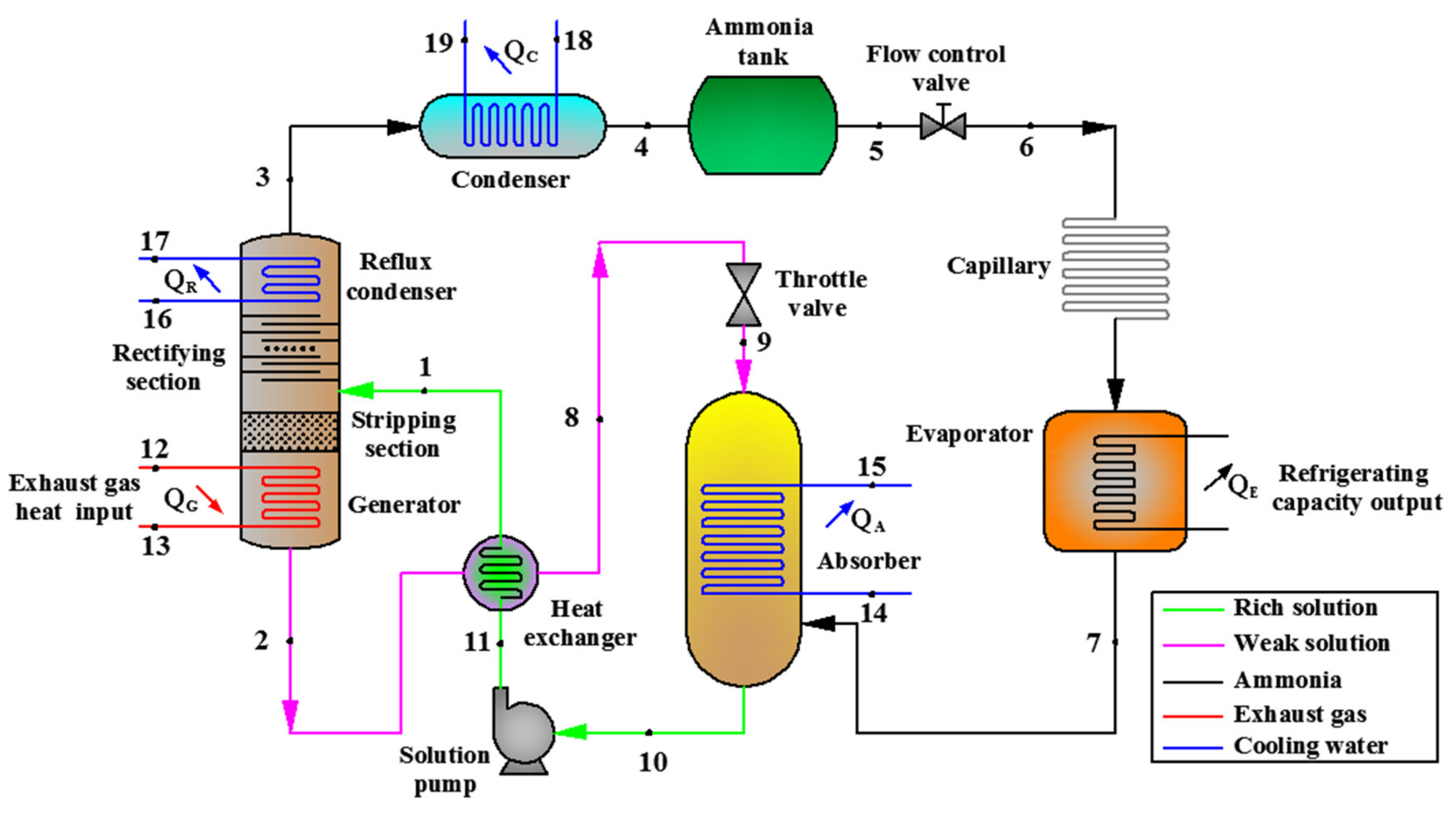
Figure 1. Schematic of the absorption refrigeration system. The key state points of the NH3-H2O-based refrigeration system operation are as follows: State point 1—rich NH3-H2O solution inlet; state point 2—weak NH3-H2O solution outlet; state point 3—ammonia vapor outlet; state points 4–6—liquid ammonia pipeline; state point 7—ammonia vapor return pipeline; state points 8 and 9—weak ammonia solution pipeline; state points 10 and 11—rich ammonia–water solution pipeline; state point 12—exhaust gas inlet; state point 13—exhaust gas outlet; state points 14, 16, and 18—cooling water inlet; state points 15, 17, and 19—cooling water outlet.
Energies 15 07070 g001
Figure 2. Schematic of the logical framework and main contents for parameter prediction.
Energies 15 07070 g002
Figure 3. Schematic of the solution strategy for prediction and control.
Energies 15 07070 g003
Figure 4. Photographs of the system’s experimental platform.
Energies 15 07070 g004
Figure 5. The structure diagrams of the three algorithms. (a) BPNN algorithm, (b) ELM algorithm, and (c) Elman algorithm.
Energies 15 07070 g005
Figure 6. Schematic of the ELM algorithm prediction procedure.
Energies 15 07070 g006
Figure 7. Predicted cooling water flow by BPNN.
Energies 15 07070 g007
Figure 8. Predicted liquid ammonia flow by BPNN.
Energies 15 07070 g008
Figure 9. Predicted cooling water flow by ELM.
Energies 15 07070 g009
Figure 10. Predicted liquid ammonia flow by ELM.
Energies 15 07070 g010
Figure 11. Predicted cooling water flow by Elman.
Energies 15 07070 g011
Figure 12. Predicted liquid ammonia flow by Elman.
Energies 15 07070 g012
Figure 13. The relationship between the predicted cooling water flow and exhaust gas.
Energies 15 07070 g013
Figure 14. The relationship between the predicted liquid ammonia flow and exhaust gas.
Energies 15 07070 g014
Figure 15. Refrigerating capacity output based on predicted parameters.
Energies 15 07070 g015
Table 1. Experimental performance of the refrigeration system.
Working FluidParameterValue
Exhaust gasInlet temperature, °C253
Outlet temperature, °C155
Flow, m3/h856
AmmoniaBefore condenser, °C42.6
After condenser, °C24.7
Generation pressure, MPa0.99
Absorption pressure, MPa0.03
Flow, m3/h18.6
Evaporation temperature, °C−22.8
Return gas temperature, °C−17.7
Rich solutionAfter absorber, °C27.8
After heat exchanger, °C116.7
Weak solutionAfter generator, °C127.9
After heat exchanger, °C43.1
Cooling waterBefore absorber, °C25
After absorber, °C26.9
Flow of absorber, m3/h12
After reflux condenser, °C42.6
Flow of reflux condenser, m3/h0.24
After condenser, °C27.2
Table 2. The selected 10 sets of measured data.
Input Exhaust Gas Temperature
°C
Exhaust Gas Flow
m3/h
Cooling Water Flow into the Absorber
m3/h
Liquid Ammonia Flow into the
Evaporator
L/h
Refrigerating Capacity
kW
25385612.018.64.75
26585612.419.14.85
27688813.119.24.86
28990213.819.34.87
29887914.519.14.80
31185615.119.04.79
32388115.919.34.87
33591716.719.54.90
35687018.119.74.93
36188118.519.44.88
Table 3. The prediction results of three different prediction algorithms.
AlgorithmThe Maximum Relative Error (%)
Cooling Water FlowLiquid Ammonia Flow
BPNN5.87.2
ELM2.55.1
Elman4.15.6
Table 4. Comparison between theoretical and experimental results.
Generation
Temperature
(°C)
Predicted Refrigeration Output
(kW)
Experimental Refrigeration Output
(kW)
The Relative Error
(%)
1256.26.03.2
1359.08.91.1
14511.310.93.5
Publisher’s Note: MDPI stays neutral with regard to jurisdictional claims in published maps and institutional affiliations.