Article

Solar Radiation Forecasting Using Machine Learning and Ensemble Feature Selection

by
Edna S. Solano
1,*,
Payman Dehghanian
2 and
Carolina M. Affonso
1
1
Faculty of Electrical Engineering, Federal University of Para, Belem 66075-110, PA, Brazil
2
Department of Electrical and Computer Engineering, The George Washington University, Washington, DC 20052, USA
*
Author to whom correspondence should be addressed.
Energies 2022, 15(19), 7049; https://doi.org/10.3390/en15197049
Submission received: 25 August 2022 / Revised: 18 September 2022 / Accepted: 22 September 2022 / Published: 25 September 2022
(This article belongs to the Special Issue AI-Based Forecasting Models for Renewable Energy Management)

Abstract

:
Accurate solar radiation forecasting is essential to operate power systems safely under high shares of photovoltaic generation. This paper compares the performance of several machine learning algorithms for solar radiation forecasting using endogenous and exogenous inputs and proposes an ensemble feature selection method to choose not only the most related input parameters but also their past observations values. The machine learning algorithms used are: Support Vector Regression (SVR), Extreme Gradient Boosting (XGBT), Categorical Boosting (CatBoost) and Voting-Average (VOA), which integrates SVR, XGBT and CatBoost. The proposed ensemble feature selection is based on Pearson coefficient, random forest, mutual information and relief. Prediction accuracy is evaluated based on several metrics using a real database from Salvador, Brazil. Different prediction time-horizons are considered: 1 h, 2 h and 3 h ahead. Numerical results demonstrate that the proposed ensemble feature selection approach improves forecasting accuracy and that VOA performs better than the other algorithms in all prediction time horizons.

Graphical Abstract

1. Introduction

Solar generation is a clean renewable energy resource that has emerged as a promising solution for reducing fossil fuel consumption and CO2 emissions. According to [1], solar energy continued globally to lead renewable capacity expansion with an increment of 133 GW (+19%) in 2021, achieving a total of 849 GW capacity and accounting for 28% of the renewable generation portfolio.
The operation of power systems with high penetration of photovoltaic (PV) generation brings about some challenges due to its non-dispatchability and intermittence, dependent on meteorological parameters and mainly cloud dynamics. The fluctuating PV generation may lead to power flow inversion with voltage and frequency variations and an imbalance between energy demand and supply; therefore, it requires the development of accurate solar radiation forecasting models for reliable power system operation.
Several forecasting models have been proposed in the literature targeting different prediction time horizons: very short-term (intra-hour), short-term (intra-day or day-ahead), medium-term (1 month) and long-term (1 year) [2], each driving different applications. For example, intra-hour and intra-day forecasting can be used for real-time power system operation. Day-ahead forecasting can be used for dispatch planning purposes. Medium and long-term forecasts can be used for maintenance and energy market purposes. Forecasting algorithms can be classified into physical models, such as Numerical Weather Prediction (NWP); statistical models, such as Autoregressive Moving Average (ARMA) and Autoregressive Integrated Moving Average (ARIMA); and data-driven models, such as Artificial Intelligence (AI) algorithms.
Physical models are based on sky images, satellite information, and mathematical equations that requires in depth understanding to describe the physical phenomena in the atmosphere [3]. Statistical models had been widely used in early works to forecast solar radiation with satisfactory results. In [4], ARMA and ARIMA models are used for short-term solar radiation forecasting. In [5], authors propose to combine an autoregressive (AR) model with a dynamical system model to 1 h-ahead solar radiation forecasting.
Over time, these models have been outperformed by techniques belonging to the field of artificial intelligence (AI) due to their ability to detect nonlinear relationships [6]. Several papers have been developed to forecast solar radiation using AI algorithms. In [7], authors compare the performance of regression and Artificial Neural Network (ANN) models to forecast solar radiation, and results show that ANN outperforms regression models. Reference [8] proposes the use of a genetic algorithm to adjust ANN parameters on a solar power forecasting model. The results are compared with ARIMA and ANN and show substantial improvements can be achieved with genetic algorithm optimization. Reference [9] proposes a hybrid model to forecast hourly solar irradiance based on self-organizing maps (SOM), support vector regression (SVR) and particle swarm optimization (PSO), and the proposed technique outperforms traditional forecasting models. More recently, researchers have used machine learning (ML) techniques to forecast solar radiation, which is a promising subfield of AI capable of dealing with a large amount of data [10]. The ML algorithms most commonly found in the literature are: support vector regression (SVR), regression tree, random forest and gradient boosting.
The forecasting model can be constructed using only endogenous inputs or with both endogenous and exogenous inputs. The endogenous input is the solar radiation time series itself, and the exogenous inputs can be the meteorological parameters that most affect the prediction, such as air temperature, humidity, wind speed, wind direction, and atmospheric pressure. A review of some recent literature on solar radiation forecasting indicates that researchers have primarily focused on developing new models and hybridizing different ML algorithms to improve forecast accuracy, mostly using as inputs past observations of solar radiation. For instance, reference [11] applies a deep learning model for solar radiation forecasting with a time horizon of 10 min and uses as input only historical observations of solar radiation. In [12], the authors propose a hybrid model for short-term solar irradiance prediction combining Long Short-Term-Memory (LSTM) and a Convolutional Neural Network (CNN), using as input the solar irradiance historical series. Reference [13] investigates the use of various deep neural network models for the one-day-ahead prediction of global horizontal irradiation (GHI) in Saudi Arabia, using only the historical values of daily GHI.
The high correlation between solar radiation and some meteorological parameters encouraged authors to use both endogenous and exogenous inputs to improve solar radiation forecasting accuracy. However, most of them perform the selection of exogenous inputs using limited algorithms such as Pearson’s correlation coefficient, which only identifies linear relationships between variables or, intuitively, by trying different combinations of input variables and choosing the one that gives the minimum forecasting error. Reference [14] proposes a solar irradiance prediction model using LSTM for three prediction horizons (1, 15 and 60 min). Two sets of input variables are considered: a complete dataset with seven meteorological data and a reduced dataset with only three meteorological data. However, the authors do not apply a feature selection methodology to adequately choose the most significant inputs. In [15], the authors propose an ensemble model for short-term PV generation forecasting combining Extreme Learning Machines (ELM), Extremely Randomized Trees (ET), k-Nearest Neighbor (KNN), Mondrian Forest (MF) and a Deep Belief Network (DBN). Several meteorological data are used as input in the forecasting model. However, the authors do not employ an input selection methodology. Reference [16] evaluates the performance of different ML algorithms for PV generation forecasting such as Linear Regression (LR), Polynomial Regression (PR), Decision Tree (DT), Support Vector Regression (SVR), Random Forest (RF), LSTM, and Multilayer Perceptron (MLP). Some meteorological parameters are used in the forecasting model, and different forecast time horizons are considered (24-h, 1 week and 1 year). In this study, input selection is performed intuitively, analyzing the relationship between each exogenous variable and the output variable.
Few studies apply a feature selection methodology for solar radiation forecasting. Reference [17] investigates the effectiveness of using exogenous inputs to perform short-term GHI forecasting with several ML models. The authors applied the following feature selection techniques: correlation, information, sequential forward selection, sequential backward selection, LASSO regression, and random forest. In [18], the authors use a hybrid ML model to perform PV power forecasting with an enhanced forward selection based on a Light Gradient Boosting decision tree (LightGBDT). In both papers, the results show that exogenous inputs improve forecasting performance.
In addition to the selection of exogenous inputs, the selection of the most related delay values (past observations) plays a key role in ensuring an effective prediction [19]. Each feature may have a temporal effect on solar radiation. For instance, some features may have a greater impact on more recent past observations, while other features may only have an impact on more distant past observations. Therefore, it is necessary to find the most relevant features and their corresponding delay value.
Few researchers have explored the optimal selection of input delay values in the solar radiation forecasting problem. This paper tries to address this knowledge gap in the literature by proposing a forecasting methodology using ML models which incorporates exogenous information and an ensemble feature selection method with an in-depth analysis to choose not only input parameters but also their delay values. The performance of several ML algorithms is investigated, and a comparative analysis is presented considering different prediction time-horizons. The ML-implemented algorithms are: Support Vector Regression (SVR), Extreme Gradient Boosting (XGBT), Categorical Boosting (CatBoost) and Voting-Average (VOA). The ensemble feature selection is based on Pearson’s coefficient, random forest, mutual Information and relief. Prediction accuracy is assessed based on several evaluation metrics. The proposed methods are tested with a real database from Salvador, Brazil.
The key contributions of this study are highlighted as follows:
  • Comparing the performance of different state-of-the-art ML algorithms, including the CatBoost algorithm, which presents fewer applications in solar radiation forecasting to the best of the authors’ knowledge;
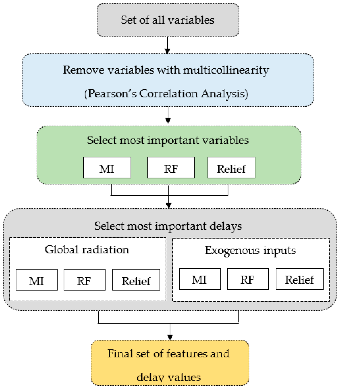
  • Proposing an ensemble feature selection method to select the most significant endogenous and exogenous variables and their delay values, integrating different ML algorithms.

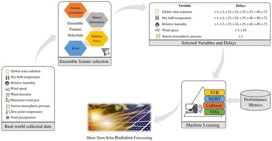
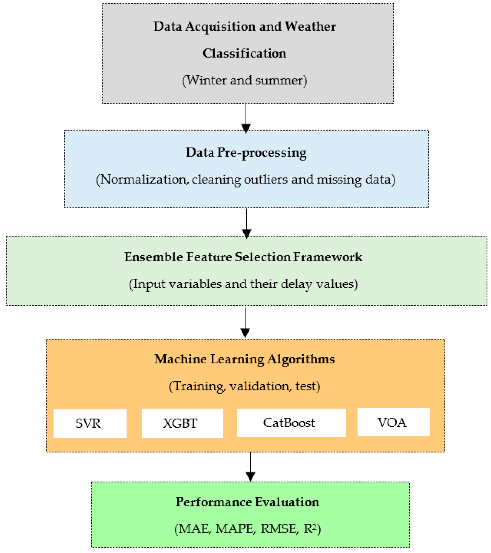
2. Proposed Methodology

The proposed approach for solar radiation forecasting includes five main steps and is presented in Figure 1. First, a real and substantial database is obtained containing data on solar radiation and other meteorological information. Then, pre-processing is performed to clean the data by removing outliers and imputing missing values. Normalization is also applied to avoid biasing toward extreme values. The next step is to select the most significant variables and their delay values, using an ensemble feature selection combining Pearson’s correlation coefficient, random forest, mutual information and relief. Then, data is separated into training, validation and test sets, and different machine learning algorithms are applied. Finally, various statistical indicators are used to quantify the accuracy of the forecasting algorithms.

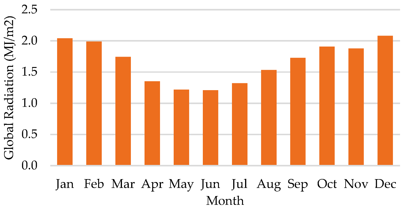
2.1. Data Description

Simulations are conducted using real-world data collected from the Brazilian National Institute of Meteorology website (INMET), which provides data from several weather stations in Brazil [20]. The referred data is from the city of Salvador, Brazil (12°58′28.9992″ S, 38°28′35.9940″ W), with hot and rainy weather all year round. Temperatures are quite stable with a minimum of 22 °C and a maximum of 31 °C. The period covered by the database is from 1 January 2015 to 3 August 2021 in sampling intervals of 1 h. Table 1 shows all variables in the database, and their statistical analysis is presented in Table 2.
Figure 2 shows the average monthly solar radiation. The dataset is divided into two periods according to the stable weather condition of the city, and different forecasting models are developed for each period. These periods are summer, from September to March, and winter, from April to August. The forecasting methodology and algorithms are implemented using Jupyter and Scikit-Learn libraries.

2.2. Pre-Processing

The pre-processing data is an important step to achieve an accurate forecasting model. First, the data needs to be cleaned from inconsistent measurements, such as missing data points and outliers [21]. In solar radiance times series, only daytime samples are considered. If the complete time series is used, many observed values are zero (night period), and the forecast values will also be zero (or very close), substantially reducing the prediction error and overestimating the performance of the forecasting model. In the other time series, missing values are replaced by applying imputation through the interpolation of the observed values. Outliers are detected using the Interquartile Range (IQR) method, which divides an ordered dataset into four quartiles (Q1, Q2, Q3, Q4), each quartile containing 25% of the data. The IQR is evaluated as the difference between Q3 and Q1, and outliers are defined as observations that fall below Q1 − 1.5 × IQR or above Q3 + 1.5 × IQR. After being identified, outliers are treated by applying interpolation, since the exclusion of these records would considerably reduce the size of the available data and affect the continuity of the hourly sampling. Min–max normalization is further applied to scale data into [0, 1].
The historical dataset is divided into three sets: training, validation and testing. The training set is used to build the ML model, with known inputs and outputs. The validation set is used to fine-tune the model hyperparameters. The testing set is used to estimate the model performance on data not used to train the model. The training set covers 70% of data with 18,521 registers from 2015 to 2019; the validation set covers 10% of data with 2629 registers from 2019 to 2020, and the test set covers 20% of data with 5299 registers from 2020, as shown in Figure 3. The validation and training sets are not continuous due to data splitting according to summer and winter seasons.

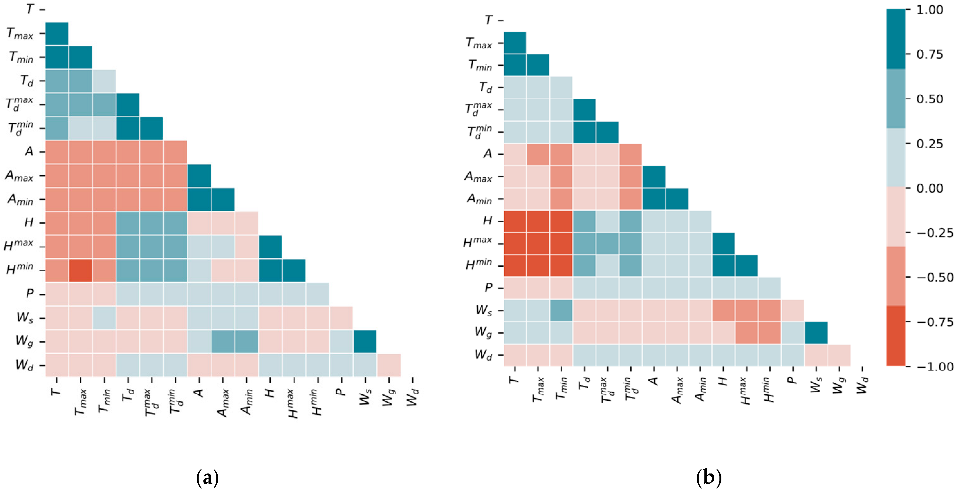
2.3. Ensemble Feature Selection

Feature selection is commonly applied in machine learning algorithms to select the best set of variables that represent the original data, thus reducing data size and model complexity and improving prediction performance [22]. Different feature selection algorithms are often tested, and the variable set with the best forecasting performance is chosen. Alternatively, an ensemble feature selection can be applied by aggregating several feature selection algorithms, combining the advantages of each one. The proposed methodology is presented in Figure 4.
The dataset used in this paper is composed of solar radiation historical series as the endogenous variable (values determined by the model) and other meteorological variables as exogenous variables (values determined outside the model). Feature selection is applied to choose the most important exogenous variables and delay values, analyzing both linear and non-linear relationships among features.
First, Pearson’s correlation analysis is performed [21]. Figure 5 shows the correlation matrix between exogenous variables for winter (a) and summer (b) seasons. A correlation coefficient r = 0 indicates that no linear relationship exists between variables, and the relationship becomes stronger as r approaches –1 or +1. As expected, results indicate a high linear correlation between variables and their minimum and maximum values. Accordingly, the following variables are removed from the dataset: hourly maximum and minimum atmospheric pressure, hourly maximum and minimum temperature, hourly maximum and minimum dew point temperature, and hourly maximum and minimum relative humidity.
An ensemble feature selection is next applied to select the most significant variables integrating the following algorithms: Mutual Information (MI), Random Forest (RF) and relief [23,24,25]. For each method, the importance of each variable is evaluated, and its value is further normalized. The final variable importance ranking is achieved by computing the mean value from different feature selection methods. The most important variables are global radiation, dry bulb temperature, relative humidity, wind speed, atmospheric pressure, and time. The threshold between the selected features and the discarded features was found empirically during the model optimization phase.
Since the dataset consists of multivariate time series, the proper selection of variable delays (past observations) is an important task to ensure acceptable forecasting accuracy. The next step is to select the delays of the endogenous and exogenous variables applying the same ensemble model. The selection of the most significant lags for the exogenous variables is done separately from the endogenous variable since they have a reduced but no weaker significance. Considering Xt − −k, a delay of k hours in variable X, the adopted range of delays to be tested is from 1 to 72 for each variable (Xt − 1 …Xt − 72), which seemed sufficient to capture important information from historical values. The final dataset with the selected variables and their delays is listed in Table 3.

3. Machine Learning Algorithms

The performance of several ML algorithms is evaluated to predict solar radiation applying the proposed methodology. The algorithms used are SVR, XGBT, CatBoost and VOA, which are briefly presented below.

3.1. Support Vector Regression (SVR)

Support Vector Regression (SVR) is an extension to the Support Vector Machine (SVM) algorithm applied to regression (predicting a continuous quantity output) instead of classification problems [26]. In basic regression models, the error is minimized, while it is fitted in SVR within a certain threshold ( ε ϵ) around the regression line (hyperplane), such that all data points within ε . are not penalized for their error.
The problem can be formulated as follows:
M i n .   1 2 w 2 + C i = 1 n ξ i .   s . a .           y i w i x i ε + ξ i   i = 1 ,   2 ,     n
where n is the number of training samples, the slack variable ξ is the deviation for any value that falls outside ε ϵ, and C is the penalty factor that determines the tradeoff between minimizing the training error and minimizing model complexity. As C increases, the tolerance for points outside ε also increases. The performance of SVR then depends on the choice of parameters ε and C .

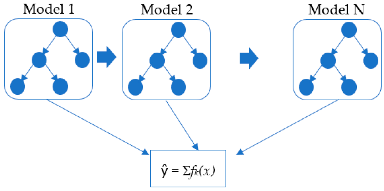
3.2. Extreme Gradient Boosting (XGBT)

Extreme gradient boosting is a decision-tree based ensemble algorithm that improves the performance of weak learners to establish an effective joint model [27]. This algorithm uses a tree ensemble model, shown in Figure 6, to predict the output.
It has been widely applied to many problems with success. In boosting, the trees are built sequentially such that each subsequent tree learns and reduces the errors of the previous one. A gradient descending algorithm is employed to minimize errors when adding new models. XGBT uses parallel processing, considerably improving the training time. It is important to mention that XGBT has a large range of hyperparameters, and their appropriate tuning is critical to the algorithm’s performance.

3.3. Categorical Boosting (CatBoost)

CatBoost is a gradient boosting framework developed by Prokhorenkova et al. [28] in 2017 and uses a binary decision-tree as base predictors. CatBoost has two main differences compared with other boosting algorithms. It uses the concept of ordered boosting, which is a random permutation approach to train the model with a subset of data while calculating residuals with another subset, thus preventing overfitting. Furthermore, the same splitting criterion is used at all nodes creating always symmetric trees. These trees are balanced and less prone to overfitting, which significantly speeds up the model execution. The CatBoost is, however, sensitive to hyperparameter tuning.

3.4. Voting Average (VOA)

Voting-averaged is an ensemble algorithm that combines the prediction from multiple ML algorithms [29]. In regression problems, VOA takes the predictions of each model and computes their average value to derive a final prediction. By combining different models, the risk of having a poor performance from one model can be mitigated by the strong performance from the other models, achieving a more robust algorithm. Since voting uses multiple ML algorithms, it is more computationally intensive. In this paper, VOA is implemented by combining: SVR, XGBT and CatBoost.

4. Performance Metrics

The performance of the algorithms is evaluated using the following error metrics: mean absolute error, mean absolute percentage error, and root mean square error. The lower the measures, the better the prediction. In the following equations, F i is the forecasted value, O i is the observed value, O ¯ i . is the mean value of observations, and n is the number of samples.
Mean absolute error (MAE):
MAE = 1 n i = 1 n F i O i
Mean absolute percentage error (MAPE):
MAPE = 1 n i = 1 n F i O i O i × 100
Root mean square error (RMSE):
RMSE = 1 n i = 1 n F i O i 2 .  
The coefficient of determination (R2) is also evaluated. It measures the variance in the predictions and varies from 0 to 1. A coefficient equal to 1 indicates that the model perfectly interprets the observed data, while a 0 indicates the model predictions perform badly on unseen data. The coefficient of determination is evaluated as follows:
R 2 = 1 i = 1 n F i O i 2 i = 1 n F i O i ¯ 2 , O ¯ i = i = 0 n 1 F i
In addition, statistical moments such as skewness (SK) and kurtosis (K) are evaluated. Skewness is a statistical measure of the asymmetry of the error distribution. It indicates the overall tendency of a forecasting model to over-forecast (in case of positive skewness) or under-forecast (in case of negative skewness). Kurtosis is a statistical measure that assesses the propensity of a distribution to have extreme (outliers) values within its tails. The excess kurtosis is a form to compare to Gaussian distribution. Since Gaussian distribution has a kurtosis of 3, excess kurtosis is evaluated by subtracting kurtosis by 3. Positive values of excess kurtosis indicate that the distribution tail is heavier and longer than Gaussian distribution, with a probability of containing more extreme values (outliers). Negative values of excess kurtosis indicate that the distribution has light tails that are shorter than Gaussian distribution and include fewer extreme values.

5. Results and Discussion

This section presents the results obtained with the proposed methodology using several ML algorithms for solar forecasting under different temporal scales. The relevance of performing an ensemble feature selection is also investigated. The hyperparameters adopted in the algorithms were selected using the GridSearchCV function from Scikit learn library [30]. It is a grid search technique that exhaustively enumerates all hyperparameter combinations and evaluates the accuracy of each combination through the validation set. Hyperparameters for both forecasting models are presented in Table 4.

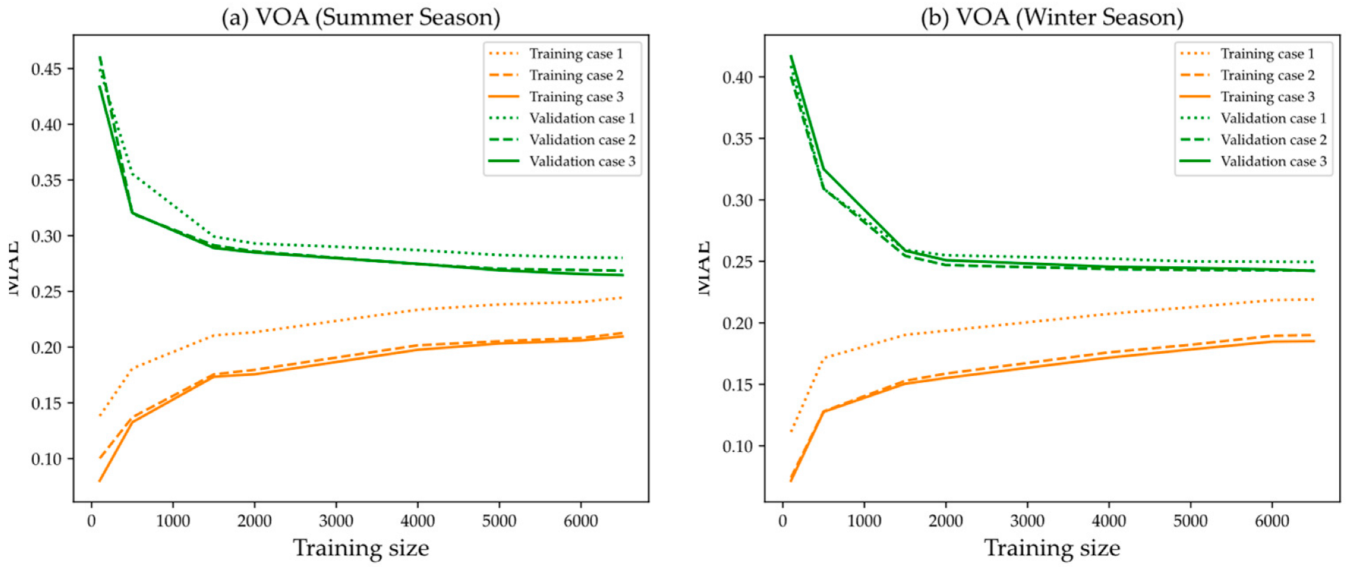
5.1. Impact of Feature Selection of Variables and Delays

In this section, the effectiveness of using an ensemble feature selection for solar radiation forecasting is investigated. Two other cases are analyzed for comparison purposes:
  • Case 1: The forecasting model is trained using only endogenous inputs, which is the solar radiation and its 10 past observations;
  • Case 2: The forecasting model is trained using both endogenous and exogenous inputs (solar radiation and other meteorological data), and their past observations are selected using the Pearson correlation coefficient;
  • Case 3: The forecasting model is trained using both endogenous and exogenous inputs, selected using the proposed ensemble feature selection.
The algorithm to perform this analysis is VOA, and for a fair comparison, the hyperparameters are kept the same in the three cases, and the models are trained and tested using the same dataset partition from the training set only. The results are presented in Table 5. Among all of them, Case 3 shows better prediction accuracy using all metrics.
Figure 7 shows the learning curve obtained with VOA for all cases. The learning curve shows the relationship between training and validation errors with a variable number of training samples. Through its analysis, it is possible to diagnose bias and variance problems in supervised learning models. In all cases, as the size of the training set increases, the training error increases and the validation error decreases, converging for a small error value, which is the desirable behavior. The narrow gap between the training and validation curves indicates a low variance error. Training data are fitted well, and the algorithm can generalize on unseen data. Case 3 has lower training and validation errors. This highlights the positive impact of applying the proposed ensemble feature and delays the selection method, which keeps the features and their significant delays that provide the most relevant information and discards features and delays that may be negatively impacting the learning process.

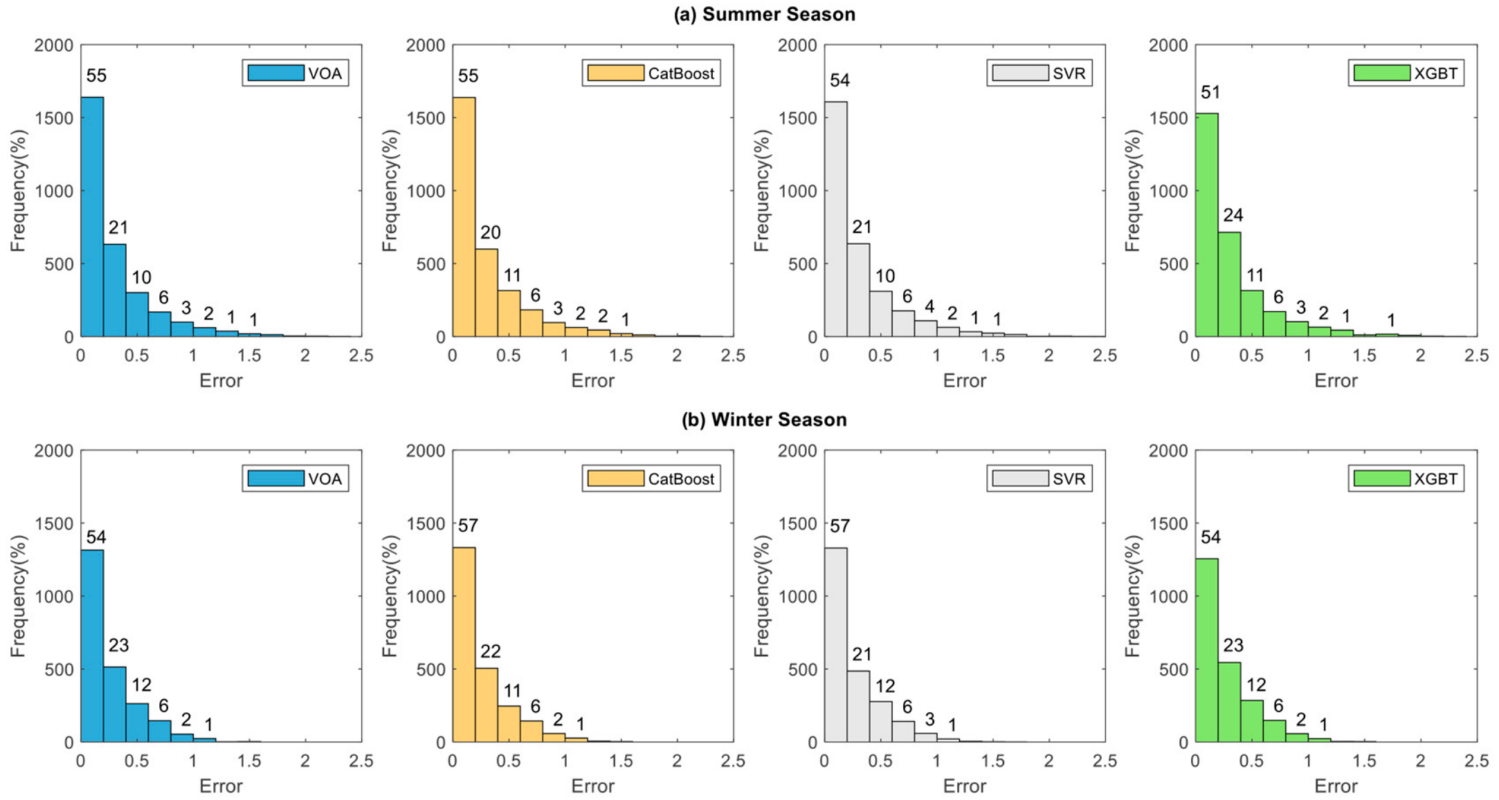
5.2. Forecasting Accuracy of Machine Learning Algorithms

This section compares the results obtained using four different ML algorithms for solar radiation forecasting with a 1-h-ahead prediction horizon. The proposed ensemble feature selection with endogenous and exogenous inputs is applied in all cases. Table 6 shows the forecasting accuracy for the test dataset in terms of MAE, RMSE, MAPE, R2, SK and K. VOA showed the best predictive performance in all metrics, except for MAPE, wherein CatBoost has a slightly lower error. XGBT presented the worst performance for all metrics during winter and summer. All models have low and positive skewness values, implying that they are more likely to forecast radiance values above rather than below the mean value. Furthermore, except for SVR during the summer season, all models exhibit negative excess kurtosis, indicating that the models are less likely to deliver extreme prediction errors.
Figure 8 shows the histogram of absolute errors obtained with each algorithm. The number of records is displayed at the top of each bin. It is possible to see that all of the ML algorithms exhibit a similar histogram. In all cases, the peak of each error distribution is centered around zero, showing that the most likely occurrence is a small solar radiation forecast error.
Figure 9 shows the solar radiation observed, forecast and the residuals obtained with the VOA algorithm during the months of winter and summer seasons, respectively. The forecasting error is larger in summer than in winter.
It is important to evaluate the computational performance of the algorithm when dealing with real-world applications. Table 7 shows the learning speed in seconds for all algorithms using summer and winter datasets, averaged over 20 runs. All of the experiments were performed on a computer with an Intel i5-1035G1 CPU (1.19 GHz) and 8.0 GByte RAM. XGBT has the lower training speed for summer and winter datasets, 2.85 s and 1.75 s, respectively. VOA has the higher training speed for summer and winter datasets, 183.93 s and 14.76 s. VOA combines SVR, XGBT and CatBoost, being more complex. All ML algorithms have a higher training speed for the summer dataset because it has more registers (data from September to March) than the winter dataset (data from April to August). All algorithms have an acceptable testing speed, with an average execution computational time of 11 s.

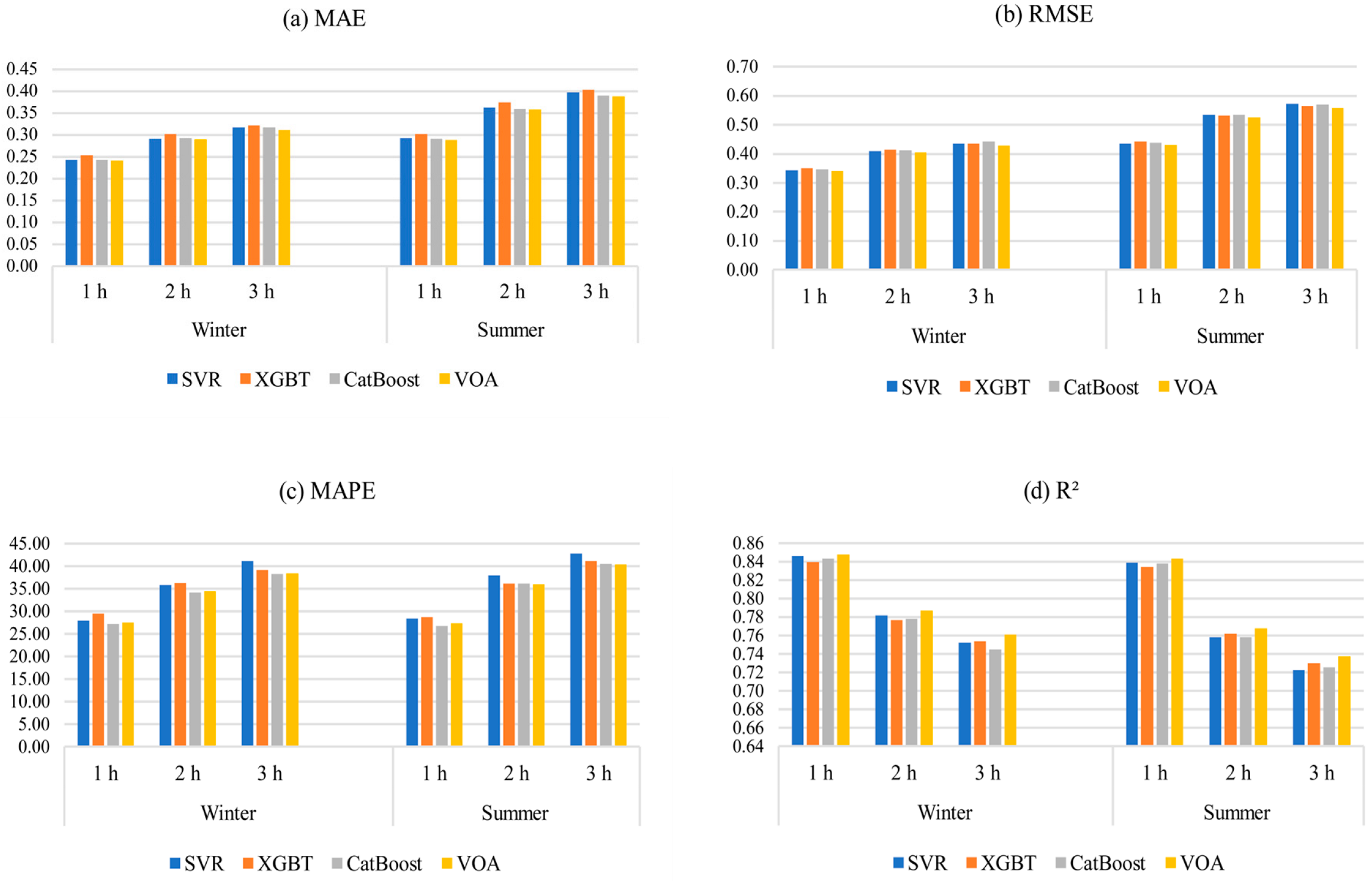
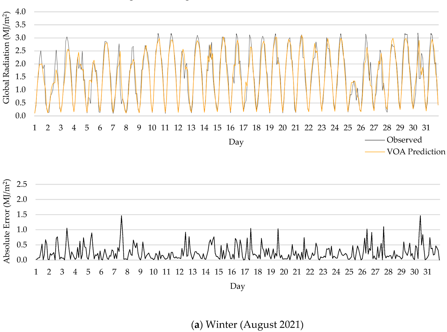
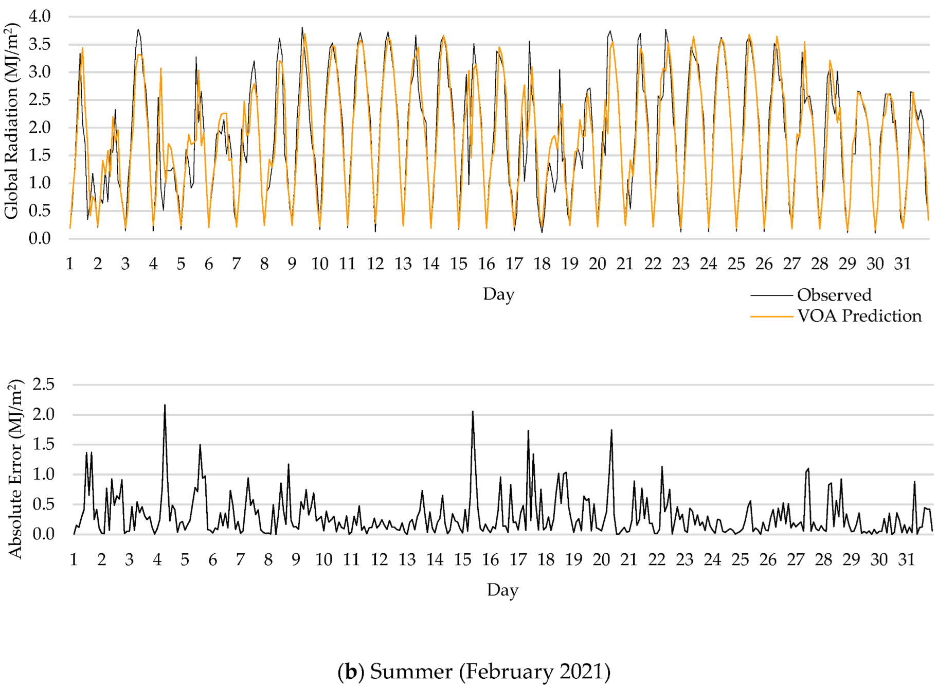
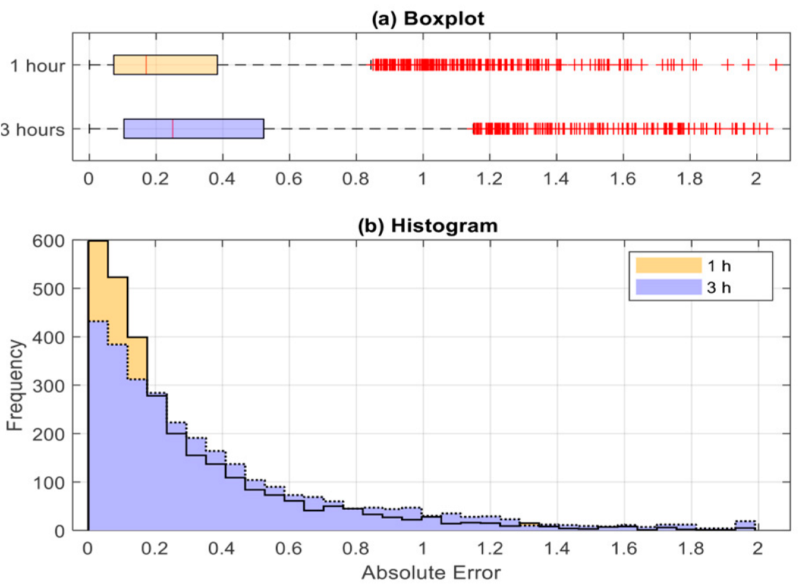
5.3. Results for Different Temporal Scales

The variability and stochasticity of photovoltaic generation usually occur on ultra-short-term and short-term time scales. Therefore, it is important to compare the effectiveness of the forecasting methodology under different temporal scales. Figure 10 shows the MAE, RMSE, MAPE and R2 for all algorithms, considering three forecasting horizons: 1 h ahead, 2 h ahead, and 3 h ahead.
As expected, as the prediction horizon increases, forecasting errors increase and R2 decreases, indicating the algorithm prediction performance degradation. Overall, the VOA demonstrated the best prediction performance among all ML algorithms used, outperforming other models in every prediction horizon, except for MAPE, wherein Catboost had the lowest error for all forecasting horizons. In most cases, XGBT presented the worst performance for a short prediction horizon (1 h), while SVR presented the worst performance for a longer prediction horizon (3 h).
Figure 11 shows the histogram and boxplot of absolute errors obtained when using VOA for the 1 h ahead and 3 h ahead forecasts. In the boxplot, the lower and upper lines denote the first and third quartile values (25th and 75th percentiles), respectively, and the median value (50th percentile) is represented by the central line. The lower and upper horizontal lines are the smallest and largest non-outliers, respectively, and outliers are represented by the ‘+’ symbol. Results show that, as the prediction horizon increases, the error distribution tail becomes fatter, and the range of error values increases. It can be concluded that the proposed methodology results in acceptable forecasting errors up to 3 h ahead, with a maximum error of 0.31 (MAE) achieved by VOA.
This study presented promising results with the proposed forecasting methodology. However, it is important to mention that, if another database from a different location needs to be used, the same methodology should be applied, but simulations must be performed to adjust the hyperparameter of the ML algorithms.

6. Conclusions

In this paper, a solar forecasting methodology is proposed using machine learning algorithms and an ensemble feature selection method. The ensemble feature selection is used to choose the most related endogenous and exogenous inputs and their past observation values and integrates Pearson’s coefficient, mutual information, random forest and relief. The advantage of the proposed feature selection method was validated comparing the obtained results against two other cases: (a) when only endogenous inputs are used and (b) when both endogenous and exogenous inputs are used, selected with Pearson’s correlation coefficient. Four state-of-the-art ML algorithms were tested to forecast solar radiation, namely SVR, XGBT, CatBoost and VOA. The performance of these algorithms was evaluated using widely adopted statistical parameters, such as MAE, RMSE, MAPE, R2, skewness and kurtosis. Three prediction time horizons were considered: 1 h, 2 h and 3 h ahead.
This study did not aim to improve the accuracy of the machine learning models used (SVR, XGBT, CatBoost and VOA) but rather to evaluate and compare their performance using different sets of inputs. The forecast methodology proposed in the present research differs from the literature by using an ensemble feature selection for choosing past observation values of both endogenous and exogenous inputs.
The main results and conclusions are summarized below:
  • The proposed ensemble feature selection outperformed the other two cases analyzed, one using only endogenous variables as inputs and the other using endogenous and exogenous variables as inputs, selected with Pearson’s correlation coefficient;
  • As the prediction horizon increased, the error distribution tail became fatter and the range of error values increased;
  • All investigated machine learning models revealed acceptable forecasting performance. Among all algorithms, VOA offered the best predictive performance, outperforming other models in every prediction horizon, except for MAPE, wherein Catboost had the lowest error for all forecasting horizons;
  • All algorithms have an acceptable testing speed for real-world applications, with an average execution computational time of 11 s. XGBT had a lower training speed, and VOA had a higher training speed.
  • One interesting finding of this research was that forecasting error was larger in summer than in winter, since the algorithms used are sensitive to the database.
In this study, the maximum number of past observations adopted in the ensemble feature selection method was chosen empirically. The results and conclusions obtained suggest that more research should be carried out for the optimal selection of this parameter, aiming to attain more accurate forecasts. Finally, as the performance of ML algorithms mainly depends on the dataset used, more experiments can be investigated using different datasets from other locations than Brazil. Besides, the proposed methodology can be applied to other forecasting problems, such as wind speed and load forecasting.

Author Contributions

Conceptualization, C.M.A. and E.S.S.; methodology, C.M.A.; software, E.S.S.; validation, C.M.A. and P.D.; formal analysis, C.M.A.; investigation, C.M.A. and E.S.S.; resources, E.S.S.; data curation, E.S.S.; writing—original draft preparation, C.M.A.; writing—review and editing, E.S.S. and P.D.; visualization, E.S.S.; supervision, C.M.A.; project administration, C.M.A.; funding acquisition, C.M.A. All authors have read and agreed to the published version of the manuscript.

Funding

This research was supported by PROPESP/UFPA and CNPq, Brazil.

Data Availability Statement

Not applicable.

Conflicts of Interest

The authors declare no conflict of interest.

References

  1. IRENA. Renewable Capacity Highlights 2022. Available online: https://www.irena.org/publications/2022/Apr/Renewable-Capacity-Statistics-2022 (accessed on 20 April 2022).
  2. Liu, C.; Li, M.; Yu, Y.; Wu, Z.; Gong, H.; Cheng, F. A Review of Multitemporal and Multispatial Scales Photovoltaic Forecasting Methods. IEEE Access 2022, 10, 35073–35093. [Google Scholar] [CrossRef]
  3. Larson, V.E. Forecasting Solar Irradiance with Numerical Weather Prediction Models. In Solar Energy Forecasting and Resource Assessment; Academic Press: Boston, MA, USA, 2013; pp. 299–318. [Google Scholar]
  4. Colak, I.; Yesilbudak, M.; Genc, N.; Bayindir, R. Multi-Period Prediction of Solar Radiation Using ARMA and ARIMA Models. In Proceedings of the 2015 IEEE 14th International Conference on Machine Learning and Applications (ICMLA), IEEE, Miami, FL, USA, 9–11 December 2015; pp. 1045–1049. [Google Scholar]
  5. Huang, J.; Korolkiewicz, M.; Agrawal, M.; Boland, J. Forecasting Solar Radiation on an Hourly Time Scale Using a Coupled AutoRegressive and Dynamical System (CARDS) Model. Solar Energy 2013, 87, 136–149. [Google Scholar] [CrossRef]
  6. Yadav, A.K.; Chandel, S.S. Solar Radiation Prediction Using Artificial Neural Network Techniques: A Review. Renew. Sustain. Energy Rev. 2014, 33, 772–781. [Google Scholar] [CrossRef]
  7. Kumar, R.; Aggarwal, R.K.; Sharma, J.D. Comparison of Regression and Artificial Neural Network Models for Estimation of Global Solar Radiations. Renew. Sustain. Energy Rev. 2015, 52, 1294–1299. [Google Scholar] [CrossRef]
  8. Pedro, H.T.C.; Coimbra, C.F.M. Assessment of Forecasting Techniques for Solar Power Production with No Exogenous Inputs. Sol. Energy 2012, 86, 2017–2028. [Google Scholar] [CrossRef]
  9. Dong, Z.; Yang, D.; Reindl, T.; Walsh, W.M. A Novel Hybrid Approach Based on Self-Organizing Maps, Support Vector Regression and Particle Swarm Optimization to Forecast Solar Irradiance. Energy 2015, 82, 570–577. [Google Scholar] [CrossRef]
  10. Voyant, C.; Notton, G.; Kalogirou, S.; Nivet, M.-L.; Paoli, C.; Motte, F.; Fouilloy, A. Machine Learning Methods for Solar Radiation Forecasting: A Review. Renew. Energy 2017, 105, 569–582. [Google Scholar] [CrossRef]
  11. Rodríguez, F.; Azcárate, I.; Vadillo, J.; Galarza, A. Forecasting Intra-Hour Solar Photovoltaic Energy by Assembling Wavelet Based Time-Frequency Analysis with Deep Learning Neural Networks. Int. J. Electr. Power Energy Syst. 2022, 137, 107777. [Google Scholar] [CrossRef]
  12. Elizabeth Michael, N.; Mishra, M.; Hasan, S.; Al-Durra, A. Short-Term Solar Power Predicting Model Based on Multi-Step CNN Stacked LSTM Technique. Energies 2022, 15, 2150. [Google Scholar] [CrossRef]
  13. Boubaker, S.; Benghanem, M.; Mellit, A.; Lefza, A.; Kahouli, O.; Kolsi, L. Deep Neural Networks for Predicting Solar Radiation at Hail Region, Saudi Arabia. IEEE Access 2021, 9, 36719–36729. [Google Scholar] [CrossRef]
  14. Wentz, V.H.; Maciel, J.N.; Gimenez Ledesma, J.J.; Ando Junior, O.H. Solar Irradiance Forecasting to Short-Term PV Power: Accuracy Comparison of ANN and LSTM Models. Energies 2022, 15, 2457. [Google Scholar] [CrossRef]
  15. Massaoudi, M.; Abu-Rub, H.; Refaat, S.S.; Trabelsi, M.; Chihi, I.; Oueslati, F.S. Enhanced Deep Belief Network Based on Ensemble Learning and Tree-Structured of Parzen Estimators: An Optimal Photovoltaic Power Forecasting Method. IEEE Access 2021, 9, 150330–150344. [Google Scholar] [CrossRef]
  16. Mahmud, K.; Azam, S.; Karim, A.; Zobaed, S.; Shanmugam, B.; Mathur, D. Machine Learning Based PV Power Generation Forecasting in Alice Springs. IEEE Access 2021, 9, 46117–46128. [Google Scholar] [CrossRef]
  17. Castangia, M.; Aliberti, A.; Bottaccioli, L.; Macii, E.; Patti, E. A Compound of Feature Selection Techniques to Improve Solar Radiation Forecasting. Expert Syst. Appl. 2021, 178, 114979. [Google Scholar] [CrossRef]
  18. Tao, C.; Lu, J.; Lang, J.; Peng, X.; Cheng, K.; Duan, S. Short-Term Forecasting of Photovoltaic Power Generation Based on Feature Selection and Bias Compensation–LSTM Network. Energies 2021, 14, 3086. [Google Scholar] [CrossRef]
  19. Surakhi, O.; Zaidan, M.A.; Fung, P.L.; Hossein Motlagh, N.; Serhan, S.; AlKhanafseh, M.; Ghoniem, R.M.; Hussein, T. Time-Lag Selection for Time-Series Forecasting Using Neural Network and Heuristic Algorithm. Electronics 2021, 10, 2518. [Google Scholar] [CrossRef]
  20. INMET. Instituto Nacional de Meteorologia. Available online: https://portal.inmet.gov.br/ (accessed on 23 October 2021).
  21. Han, J.; Kamber, M.; Pei, J. Data Mining: Concepts and Techniques, 3rd ed.; Elsevier Inc.: Waltham, MA, USA, 2012. [Google Scholar]
  22. Mera-Gaona, M.; López, D.M.; Vargas-Canas, R.; Neumann, U. Framework for the Ensemble of Feature Selection Methods. Appl. Sci. 2021, 11, 8122. [Google Scholar] [CrossRef]
  23. Shannon, C. A mathematical theory of communication. Bell Syst. Tech. J. 1948, 27, 379–423. [Google Scholar] [CrossRef]
  24. Breiman, L. Random forests. Mach. Learn. 2001, 45, 5–32. [Google Scholar] [CrossRef]
  25. Kira, K.; Rendell, L. A Practical Approach to Feature Selection. Mach. Learn. Proc. 1992, 1992, 249–256. [Google Scholar] [CrossRef]
  26. Shalev-Shwartz, S.; Ben-David, S. Understanding Machine Learning: From Theory to Algorithms, 1st ed.; Cambridge University Press: New York, NY, USA, 2014. [Google Scholar]
  27. Chen, T.; Guestrin, C. XGBoost: A Scalable Tree Boosting System. In Proceedings of the 22nd ACM SIGKDD International Conference on Knowledge Discovery and Data Mining, San Francisco, CA, USA, 13–17 August 2016. [Google Scholar]
  28. Prokhorenkova, L.; Gusev, G.; Vorobev, A.; Dorogush, A.; Gulin, A. CatBoost: Unbiased boosting with categorical features. In Proceedings of the 32nd International Conference on Neural Information Processing Systems, Montréal, QC, Canada, 3 December 2018. [Google Scholar]
  29. An, K.; Meng, J. Voting-Averaged Combination Method for Regressor Ensemble. In Advanced Intelligent Computing Theories and Applications; Huang, D.S., Zhao, Z., Bevilacqua, V., Figueroa, J.C., Eds.; Springer: Berlin/Heidelberg, Germany, 2010; Volume 6215, pp. 540–546. [Google Scholar]
  30. Agrawal, T. Hyperparameter Optimization Using Scikit-Learn. In Hyperparameter Optimization in Machine Learning; Apress: Berkeley, CA, USA, 2021; pp. 31–51. ISBN 978-1-4842-6578-9. [Google Scholar]
Figure 1. Flowchart of the proposed methodology.
Energies 15 07049 g001
Figure 2. Average monthly solar radiation from January 2015 to August 2021 in Salvador, Brazil.
Energies 15 07049 g002
Figure 3. Training, validation and testing set of solar radiation historical series.
Energies 15 07049 g003
Figure 4. Ensemble feature selection methodology.
Energies 15 07049 g004
Figure 5. Correlation matrix: (a) winter season and (b) summer season.
Energies 15 07049 g005
Figure 6. Tree ensemble model for boosting algorithms.
Energies 15 07049 g006
Figure 7. Learning Curves for VOA. (a) Summer season. (b) Winter season.
Energies 15 07049 g007
Figure 8. Histogram of the absolute error for all ML algorithms. (a) Summer. (b) Winter.
Energies 15 07049 g008
Figure 9. Solar radiation observed, forecast and residuals for 1 h ahead using VOA: (a) winter and (b) summer.
Energies 15 07049 g009aEnergies 15 07049 g009b
Figure 10. Performance of ML algorithms for different prediction time horizons: (a) MAE, (b) RMSE, (c) MAPE, (d) R2.
Energies 15 07049 g010
Figure 11. Absolute error using VOA to forecast 1 h ahead and 3 h ahead: (a) histogram and (b) boxplot.
Energies 15 07049 g011
Table 1. Available database for solar radiation forecasting.
DataAbbreviationUnity
HourHhour
Global solar radiationRMJ/m2
Maximum wind gustWgm/s
Wind speedWsm/s
Wind directionWd°
Dry bulb temperatureT°C
Hourly maximum temperatureTmax°C
Hourly minimum temperatureTmin°C
Dew point temperatureTd°C
Hourly maximum dew point temperatureTdmax°C
Hourly minimum dew point temperatureTdmin°C
Total precipitationPmm
Station atmospheric pressureAmb
Hourly maximum atmospheric pressure Amaxmb
Hourly minimum atmospheric pressureAminmb
Relative humidity H%
Hourly maximum relative humidityHmax%
Hourly minimum relative humidityHmin%
Table 2. Statistical features of the available database.
VariableMeanStandard DeviationMinMax
H12.03.16237.017.0
R1.65331.04620.00094.15
Wg5.66511.73020.600010.6
Ws1.60690.53720.13.0
Wd130.801759.75261.0360.0
T27.36082.406920.434.2
Tmax28.14142.518120.835.8
Tmin26.50072.370819.932.4
Td21.53681.481216.825.5
Tdmax22.28971.470817.326.0
Tdmin20.85311.482016.325.1
P0.20411.34190.050.4
A1009.40622.96361001.61017.7
Amax1009.71372.92761001.91018.1
Amin1009.21022.92651001.41017.5
H71.324010.471145.096.0
Hmax75.056610.135952.097.0
Hmin68.114911.013338.096.0
Table 3. Selected set of input variables and delay values.
Winter
VariableDelays
Global solar radiationt − 1, t − 2, t − 23, t − 24, t − 25, t − 47, t − 48, t − 72
Dry bulb temperaturet − 1, t − 2, t − 23, t − 24, t − 25, t − 48, t − 49, t − 72
Relative humidity t − 1, t − 2, t − 23, t − 24, t − 25, t − 48, t − 49, t − 72
Wind speedt − 1, t − 24
Atmospheric pressure t − 2
Hour, day, month-
Summer
VariableDelays
Global solar radiationt − 1, t − 2, t − 23, t − 24, t − 25, t − 47, t − 48, t − 72
Dry bulb temperaturet − 1, t − 2, t − 23, t − 24, t − 25, t − 48, t − 49, t − 72
Relative humidity t − 1, t − 2, t − 23, t − 24, t − 25, t − 48, t − 49, t − 72
Wind speedt − 1, t − 2
Atmospheric pressure t − 3
Hour, day, month-
Table 4. Algorithm hyperparameter tuning.
AlgorithmHyperparameter
WinterSummer
SVRregularization C = 10, ε = 0.01, γ = auto, kernel function K = RBFRegularization C = 100, ε = 0.001, γ = auto, kernel function K = RBF
XGBTlearning rate = 0.1, max. depth = 5, number of estimators = 80, subsample = 0.9learning rate = 0.1, max. depth = 5, number of estimators = 100, subsample = 0.8
CatBoostdepth = 6, L2 regularization = 10, learning rate = 0.05, iterations = 2000depth = 6, L2 regularization = 10, learning rate = 0.05, iterations = 2000
VOAXGBT (learning rate = 0.1, max. depth = 5, number of estimators = 80, subsample = 0.9)
CatBoost (depth = 6, L2 regularization = 10, learning rate = 0.05, iterations = 2000)
SVR (regularization C = 10, ε = 0.01, γ = auto, kernel function K = RBF)
XGBT (learning rate = 0.1, max. depth = 5, number of estimators = 100, subsample = 0.8)
CatBoost (depth = 6, L2 regularization = 10, learning rate = 0.05, iterations = 2000)
SVR (regularization C = 100, ε = 0.001, γ = auto, kernel function K = RBF)
Table 5. Comparison of forecasting performance for different input datasets using VOA.
Winter
Input SetMAERMSEMAPER2
Case 1: endogenous0.25910.353234.19550.8377
Case 2: end + exog (Pearson coefficient)0.25210.343932.86270.8460
Case 3: endo + exog (ensemble selection)0.25370.343131.89280.8468
Summer
Input SetMAERMSEMAPER2
Case 1: endogenous0.31530.453635.41390.8261
Case 2: end + exog (Pearson correlation)0.30170.435831.14110.8395
Case 3: endogenous and exogenous0.3030.432630.61060.8417
Table 6. Forecasting accuracy of ML algorithms (1 h ahead).
Winter
SVRXGBTCatBoostVOA
MAE0.24300.25340.24260.2417
RMSE0.34330.35070.34700.3418
MAPE28.012229.535027.216327.4862
R20.84660.83990.84330.8480
SK0.13360.08800.09940.1039
K−1.1632−1.1829−1.2022−1.1877
Summer
SVRXGBTCatBoostVOA
MAE0.29220.30090.29050.2877
RMSE0.43660.44260.43730.4309
MAPE28.359028.695126.812727.3177
R20.83890.83440.83830.8430
SK0.04620.03320.03380.0360
K0.2922−1.1663−1.1551−1.1563
Table 7. Average learning speed in seconds (s) for all ML algorithms (1 h ahead).
Learning Speed (s)
SVRXGBTCatBoostVOA
Summer63.092.8513.08183.93
Winter9.731.759.8114.76
Testing Speed (s)
Summer36.991.4413.3513.14
Winter4.911.1710.2710.58
Publisher’s Note: MDPI stays neutral with regard to jurisdictional claims in published maps and institutional affiliations.

