Analytical Solution of Heat Transfer Performance of Grid Regenerator in Inverse Stirling Cycle

Abstract

The regenerator plays an extremely important role in the Stirling circulation. A grid regenerator can be used for inverse Stirling machines at room temperature due to its low flow resistance. This paper proposes a hexagonal grid regenerator to theoretically explore heat transfer properties in the inverse Stirling cycle and establishes an approximate analytical model to analyze the effect mechanism of working frequency, thermal diffusivity and wall thickness on the oscillation flow. The results show that the wall thickness is one of the key factors affecting the equivalent heat transfer coefficient. Specifically, too small or too large wall thickness increases the instability of the heat transfer process. The ultimate wall thickness is determined by the equivalent heat transfer coefficient and thermal penetration depth, whose optimal value ensures not only sufficient heat exchange but also the full utilization of materials. With the increase in frequency, heat exchange performance is improved monotonously. Therefore, high–frequency operation can improve the heat exchange performance of the regenerator. In addition, an optimization criterion for the size of regenerator with the specific capacity of heat transfer as the objective parameter is proposed based on the equivalent heat transfer coefficient. The optimal parameters were obtained when relative thickness was set as 0.8 mm and the equivalent heat transfer coefficient was up to 10⁴–10⁵ W/m²·K indicating that the grid regenerator has broad application prospects in the inverse Stirling cycle.

1. Introduction

The refrigeration and heating of the inverse Stirling cycle at room temperature has been proved to have the advantages of energy saving, environmental protection and high efficiency and has always been one of the focuses of research. Compared with steam compression cycle technology, inverse Stirling cycle technology does not use a refrigerant and does not emit carbon dioxide. It is a perfect alternative to sustainable technologies in the future. At the same time, the theoretical efficiency of the inverse Stirling cycle is equivalent to the efficiency of the Carnot cycle, which is the maximum possible efficiency of any engine cycle technology under the specific temperature limit operation, which is unmatched by other technologies. For instance, the use of inverse Stirling cycle technology to develop air–conditioning compressors for pure electric vehicles has outstanding technical advantages; efficient and environmentally friendly inverse Stirling air conditioning technology is an important issue to overcome the short battery range of pure electric vehicles [1,2,3]. Hachem et al. studied a Stirling machine at room temperature and under normal pressure with air as the working medium. Their results show that the machine achieved the bi–directional function of cooling/heating by driving a crank slider mechanism and rotating counterclockwise/clockwise with the help of a motor [4,5]. Haywood studied the inverse Stirling cycle technology at ambient temperature (−233–313 K) and modified the Stirling engine with a 4α double–acting structure to provide the bi–directional function of heating and cooling. The COP value of the Stirling machine was up to 4.5 when the temperature at hot and cold ends was 293 K and 278 K, respectively [6].

The heat exchange performance of the regenerator, a key unit of energy conversion in Stirling cycle, has the most significant impact on the Stirling engine efficiency [7]. The temperature difference between hot and cold chambers of the Stirling engine is mostly more than 500 K. For instance, the temperature ratio of the two chambers of 40 HP and 4–235 engines is 691 K/71 K and 683 K/43 K, respectively. The temperature of the hot chamber at the Stirling heat pump at room temperature ranges from 290 K to 350 K, while that of the cold chamber from −250 K to 280 K, with a difference between the two of less than 100 K [8]. Compared with incomplete heat loss and axial thermal conductivity loss, the loss of flow resistance pressure drop can be ignored, while that of loss cannot [9].

The regenerator can be in the form of screen type [10], packing type [11], porous medium [12], parallel plate [13], pin–array stack [14,15], etc. Some new types of regenerators are also being developed, such as a novel freeze–cast regenerators [16].

At present, research mostly focuses on screen or packing regenerators, which have strong heat storage capacity but high flow resistance [17]. York found that no matter what stacking method was adopted, the average misalignment rate was 44–49%, and that flow resistance was mainly caused by such misalignment [18]. Dellali et al. experimentally studied the pressure, pressure drop, speed and friction coefficient of the pin–array stack regenerator under the condition of reciprocating flow, and found that pressure drop was related to frequency and might be mainly caused by the viscous effect arising from the increased speed with the increase in frequency [19]. Yuan et al. investigated the frequency–dependent heat transfer characteristics of the magnetothermal regenerator of the parallel plate and found that, different from steady–state flow, the convective heat transfer coefficient in the matrix of the parallel plate depended not only on the fluid velocity but also the operating frequency due to the oscillating flow in the regenerator. Compared with steady–state flow, the heat transfer coefficient varies from −17% to 68% [20]. Pan proposed a novel method to calculate the pressure drop loss in the regenerator of a VM refrigerator, and pointed out that the pressure drop loss in the regenerator would reduce refrigeration capacity in two ways: one was friction, that is, the pressure drop in the regenerator would be converted into heat, directly reducing refrigeration capacity, and the other was pressure drop in the regenerator that would reduce the pressure ratio at the cold end [21]. The advantage of pin–array stack regenerators can be more available for high frequencies, but in thermoacoustic engines and pulse tube refrigerators only [22].

Existing regenerators cannot meet the requirements of small temperature difference and low flow resistance, so it is necessary to design and develop a new type of regenerator to make the pressure drop small when the gas passes by while possessing excellent heat exchange performance [23]. Wang et al. developed a hexagonal tube grid regenerator based on additive manufacturing technology to reduce the flow resistance by 96.2% compared with screen regenerators under the same condition. Meanwhile, the accuracy of the theoretical analysis method under the condition of single blowing was verified by combining simulation and experimental methods [9,10,11,12,13,14,15,16,17,18,19,20,21,22,23,24]. Many studies focus on the optimization of wire diameter size of a wire mesh regenerator. For example, Boroujerdi et al. proposed a new relationship between heat transfer and pressure drop characteristics of a wire mesh regenerator to calculate the oscillating flow. According to the deduced relation, the thinner the wire, the greater the pressure drop and the higher the heat transfer rate [25]. At the same time, there are also some questionable suggestions on the selection of regenerative material. Compared with traditional metal materials, a rotary regenerator made of polymer is light in weight and has strong corrosion resistance, which can reduce the operating cost and maintenance time of the thermal system [26].

To sum up, there is little research on regenerators with small temperature difference and low flow resistance. The hexagonal tube grid regenerator (HTGR) proposed in this paper is a novel regenerator with small temperature difference and low flow resistance, which has been granted an invention patent (authorization number ZL202110300042.7). Its structural characteristics are similar to those of the circular tube bundle and the pin–array structure, but the geometric structure has better uniformity, which can reduce the flow resistance and make full use of the heat storage capacity of solid materials. The existing research gap is that the influence law of oscillatory flow frequency, solid material, structure size and wall thickness on the heat transfer performance of the HTGR is not clear at present. The idea for addressing these research gaps is: according to the structural characteristics of the HTGR, an approximate geometric model is established according to the theory of heat conduction, the analytical solution is further derived, and the numerical verification is carried out based on the N–S equation. The objective of this study is to reveal the temperature distribution and heat transfer performance of the HTGR under oscillating flow. According to the parameters of oscillating flow frequency, solid material, structure size and wall thickness, the optimal design procedure of the HTGR is then established.

Aiming at the above problems, this paper focuses on the heat conduction law, such as the equivalent heat transfer coefficient (EHTC) of temperature distribution, by taking oscillation frequency, grid geometry, and material thermal diffusivity as the variable, and finally determines the optimal design mainly from the following perspectives:

• According to the heat conduction theory under periodic boundary conditions, an analytical expression of temperature distribution in a single grid is established.
• The influence of oscillation frequency, grid geometry, material thermal diffusivity and other parameters on temperature distribution and EHTC is discussed to further demonstrate the superiority of the HTGR in the inverse Stirling cycle at room temperature.
• Taking the maximum specific volume heat transfer capacity (SVHTC) as the objective function and the oscillation frequency, grid geometry and material thermal diffusivity as variables, the methods for identifying the optimal solution are explored.

This work provides theoretical guidance and reference for the design and operation of an HTGR. This paper is structured as follows: Section 1 describes the current situation and main problems of regenerators used at room temperature at home and abroad; Section 2 simplifies the physical model of the HTGR; in Section 3, the one–dimensional quasi–steady temperature field of a single circular tube in cylindrical coordinates is solved and its analytical expression is obtained; and Section 4 studies the temperature distribution and its influencing factors, analyzes the heat transfer coefficient under oscillation [27], discusses the optimization of circular tube thickness under specific surface area, and finally gives the conclusion of this paper.

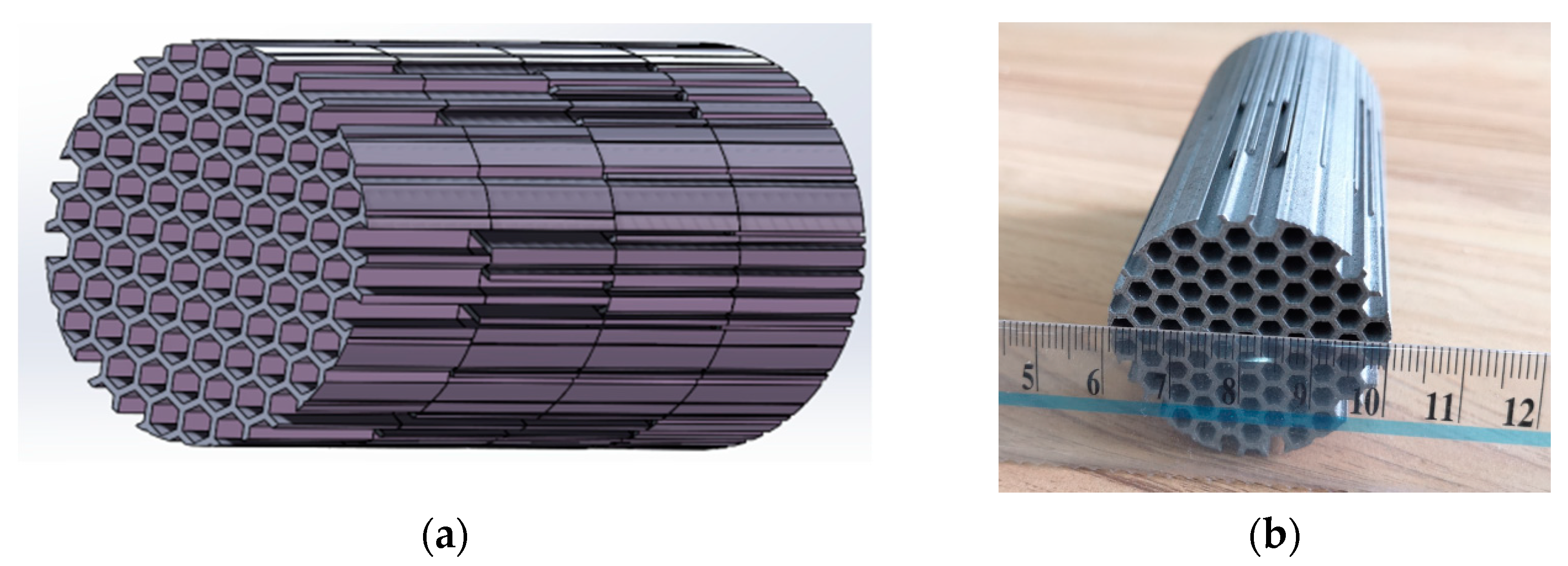
2. Physical Model of HTGR

An HTGR that met the requirements in small temperature difference and low flow resistance is designed based on additive manufacturing technology [9,10,11,12,13,14,15,16,17,18,19,20,21,22,23,24], whose geometric model is shown in Figure 1.

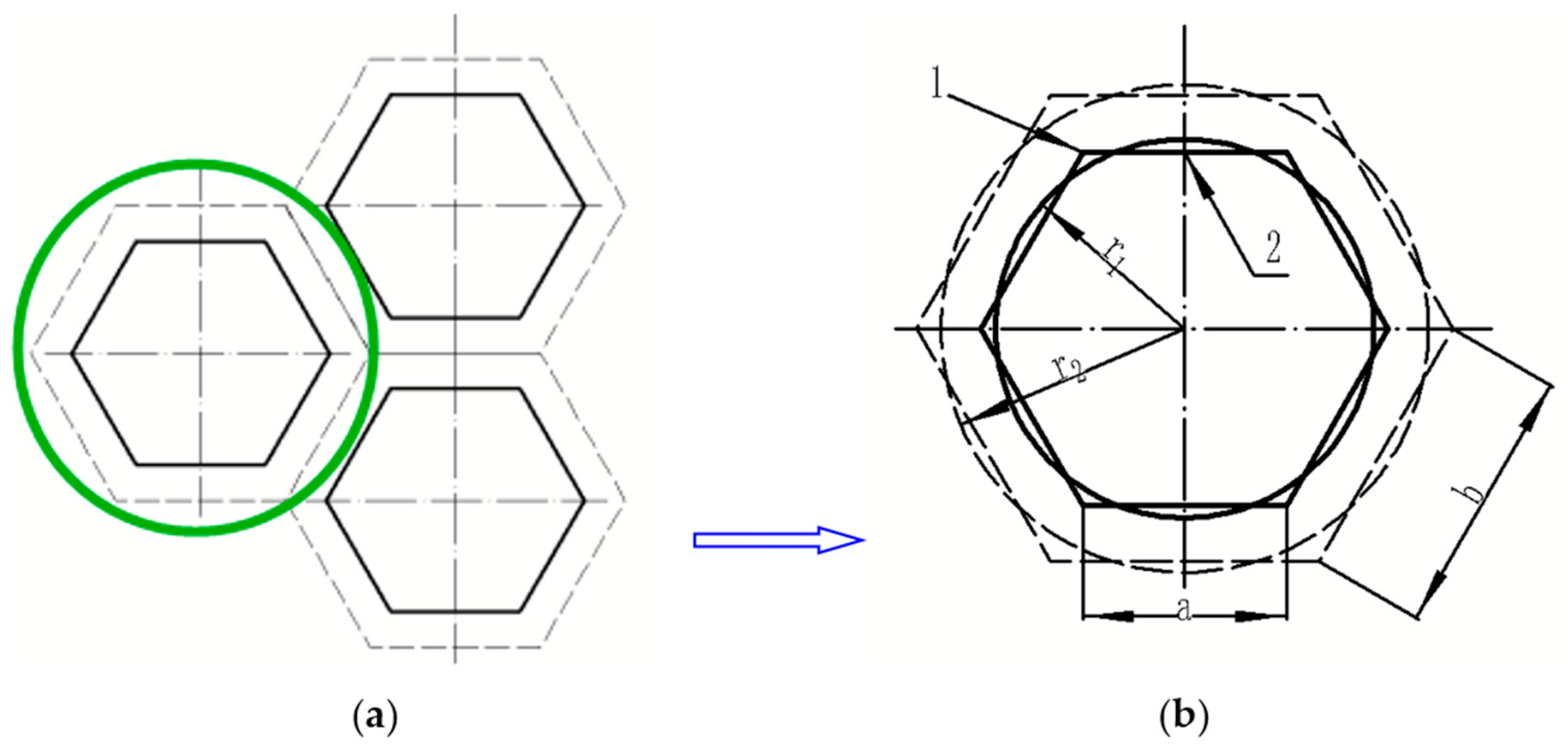
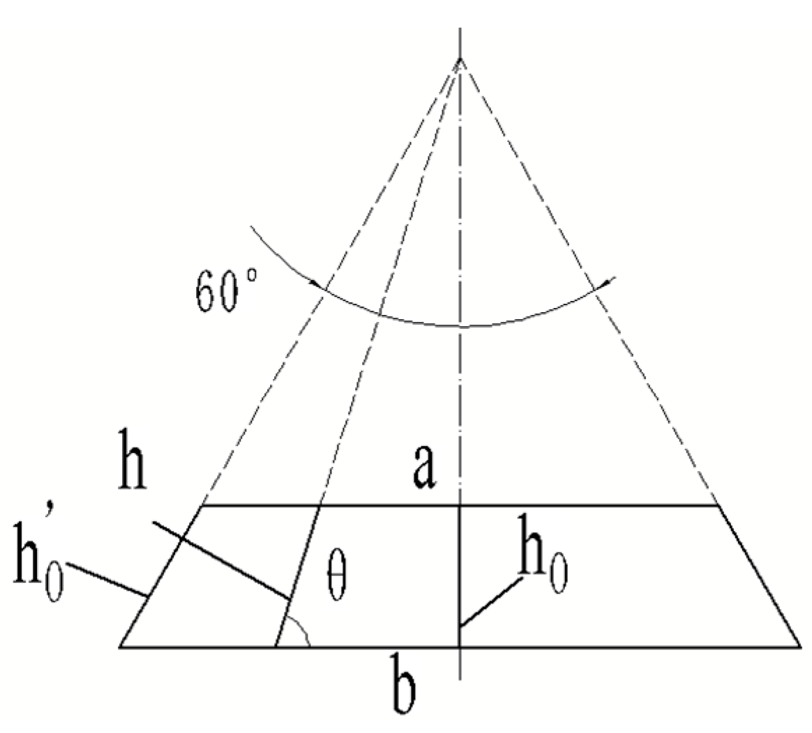
The grid is shaped like a hexagonal straight tube, which is a complex structure. In order to build an analytical model, the physical model of the grid was simplified. One of the grids was selected for research, and the regular hexagonal tube was equivalently converted into a circular tube, as shown in Figure 2. Figure 2a is the local section shape of the HTGR and Figure 2b is the physical model of a single grid. The heat exchange boundary of the inner tube wall is indicated by a solid line and the adiabatic boundary by the symmetric center line, or dotted line.

Assuming that the inner side length of the regular hexagonal tube is a, the outer length is b, the inner diameter of the circular tube is r₁, and the outer diameter is r₂, then the geometry of the equivalent transformation between the regular hexagonal tube and the circular tube is essentially the geometric space transformation between the inner and outer lengths of the hexagonal tube (a, b) and the inner and outer radius of the circular tube (r₁, r₂). Since the main function of a regenerator is to store and release heat by means of frequent heat transfer between the wall surface and thickness, the equivalent conditions should be: (1) heat transfer areas are equal to ensure the same heat transfer; (2) the volume–specific surface areas are equal to ensure the same heat storage.

The heat exchange area per unit tube length is equal:

$$2\pi r_1=6a$$

(1)

The wall thickness of the unit tube length is equal to the volume:

$$\pi (r_2^2-r_1^2)=3(b^2-a^2)\sin (\frac{\pi }{3})$$

(2)

Thus, the thermal conductivity of the HTGR can be studied by replacing the hexagonal tube with a circular tube (as shown in Appendix A).

A simplified model of a single circular tube is shown in Figure 3. Assumptions are made as follows:

(1)

The temperature field is distributed in the circumferential direction of the tube, so the problem is simplified to a two–dimensional problem in the axial and radial directions, and the model is symmetrical in the axial direction. The temperature distribution is expressed as T(r,z,t), where r is the radius and r₁ ≤ r ≤ r₂, t is the time and t ≥ 0.

(2)

To explore the mechanism of radial heat transfer, it is assumed that the length of circular tube Z is far greater than r₂, and that the influence of axial Z heat conduction is negligible; then, the temperature distribution could be simplified as T(r,t).

(3)

At each axial position Z, the temperature of the fluid changes periodically with respect to a certain equilibrium temperature, which constitutes the boundary condition of heat transfer in a circular tube.

Figure 3. Simplified model of a single circular tube.

Figure 3. Simplified model of a single circular tube.

Since a Stirling machine regenerator works by continuously exchanging compression and expansion, assuming that the temperature distribution observed the law of cosine periodic change, then the boundary conditions of the inner wall r = r₁ at each position Z can be written as:

$$T(Z)=T_{0,z}+A\cos (\omega t)$$

(3)

where T_0,z is the average temperature fluctuation at each axial position Z of the regenerator, and ω is the circular frequency of temperature fluctuation, whose relationship with the working frequency f can be expressed as:

$$\omega =2\pi f$$

(4)

3. Mathematical Model and Its Solution

Based on hypothesis (1), the governing equation of the above physical model is the unsteady heat conduction equation in a cylinder, which can be expressed as Equation (5) in a cylindrical coordinate system [28]:

$$\frac{{\partial }^{2}T}{\partial r^2}+\frac{1}{r}\frac{\partial T}{\partial r}+\frac{{\partial }^{2}Z}{\partial z^2}=\frac{1}{\alpha }\frac{\partial T}{\partial t}$$

(5)

Based on hypothesis (2), and given that the influence of axial heat conduction is ignored, the equation can be simplified into:

$$\frac{{\partial }^{2}T}{\partial r^2}+\frac{1}{r}\frac{\partial T}{\partial r}=\frac{1}{a}\frac{\partial T}{\partial t}$$

(6)

The problem is further simplified as one–dimensional unsteady heat conduction along radial r, and the boundary conditions satisfy Equations (7) and (8):

The boundary conditions of the inner circle are of the first type, which is non–homogeneous:

$$r=r_1, T=T_{0,Z}+A\cos (\omega t)$$

(7)

The boundary condition of the outer circle is of the second type, which is homogeneous:

$$r=r_2,\frac{\partial T}{\partial r}=0$$

(8)

where r₁ and r₂ are the inner and outer diameters of the circular tube. When the Stirling machine is working stably, the temperature at each position in the tube would change periodically with the same frequency as the boundary condition, and the average temperature would be the same as the boundary condition.

The difference between the temperature at each location and its mean is defined as θ; then, $\theta (r,t)=T-T_{0,z}$. Hence, the original problem is transformed into:

$$\frac{{\partial }^2\theta }{\partial r^2}+\frac{1}{r}\frac{\partial \theta }{\partial r}=\frac{1}{\alpha }\frac{\partial \theta }{\partial t}$$

(9)

The corresponding boundary conditions become:

$$r=r_1, \theta =A\cos (\omega t)$$

(10)

$$r=r_2, \frac{\partial \theta }{\partial r}=0$$

(11)

To solve the problem constituted by Equation (9) and its boundary conditions (10) and (11), it can be assumed that:

$$\theta (r,t)=\mathrm{Re}\left[\mathrm{R}\right(r{)\mathrm{e}}^{i\omega t}]$$

(12)

In order to separate the time and space variables of the governing equation, the solution in the form of a complex function is:

$$\mathrm{w}(r,t)=R(r{)\mathrm{e}}^{i\omega t}$$

(13)

Substituted into the governing Equation (9), we can obtain R© from:

$$\frac{d^{2}R}{d{r}^2}+\frac{1}{r}\frac{dR}{dr}=i\frac{\omega }{\alpha }R$$

(14)

The corresponding boundary conditions of Equation (14) are:

$$r=r_1, R(r_1)=A$$

(15)

$$r=r_2, \frac{dR}{dr}=0$$

(16)

Equation (14) is a typical zero–order Bessel equation. Let $\beta =\sqrt{\raisebox{1ex}{$\omega $}\!\left/ \!\raisebox{-1ex}{$\alpha $}\right.}$; the general solution is [29]:

$$R(r)=B{J}_0(\sqrt{-i}\beta r)+C{Y}_0(\sqrt{-i}\beta r)$$

(17)

where $J_0(\sqrt{-i}\beta r)$ is a zero–order Bessel function of the first kind, $J_0(\sqrt{-i}\beta r)$ is a zero–order Bessel function of the second kind, and B and C are undetermined constants determined by boundary conditions.

B and C are solved by:

$$B=-\frac{A{Y}_1(\sqrt{-i}\beta r_2)}{Y_0(\sqrt{-i}\beta r_1)J_1(\sqrt{-i}\beta r_2)-Y_1(\sqrt{-i}\beta r_2)J_0(\sqrt{-i}\beta r_1)}$$

(18)

$$C=\frac{A{J}_1(\sqrt{-i}\beta r_2)}{Y_0(\sqrt{-i}\beta r_1)J_1(\sqrt{-i}\beta r_2)-Y_1(\sqrt{-i}\beta r_2)J_0(\sqrt{-i}\beta r_1)}$$

(19)

Substituting B and C into Equation (17), we obtain ©(r) as:

$$R(r)=\frac{A(J_1(\sqrt{-i}\beta r_2)Y_0(\sqrt{-i}\beta r)-Y_1(\sqrt{-i}\beta r_2)J_0(\sqrt{-i}\beta r))}{Y_0(\sqrt{-i}\beta r_1)J_1(\sqrt{-i}\beta r_2)-Y_1(\sqrt{-i}\beta r_2)J_0(\sqrt{-i}\beta r_1)}$$

(20)

Substituting Equation (20) into Equation (13), we can obtain θ(r,t) as:

$$\theta (r,t)=T-T_{0,z}=\mathrm{Re}\left[\mathrm{R}\right(r{)\mathrm{e}}^{i\omega t}]=\left|R(r)\right|\cos (\omega t-\varphi (r))$$

(21)

where $\left|R(r)\right|$ is the amplitude, noted ©©(r), and ϕ(r) is the phase angle. They are, respectively, expressed as:

$$A_r(r)=\left|R(r)\right|=A\left|\frac{(J_1(\sqrt{-i}\beta r_2)Y_0(\sqrt{-i}\beta r)-Y_1(\sqrt{-i}\beta r_2)J_0(\sqrt{-i}\beta r))}{Y_0(\sqrt{-i}\beta r_1)J_1(\sqrt{-i}\beta r_2)-Y_1(\sqrt{-i}\beta r_2)J_0(\sqrt{-i}\beta r_1)}\right|$$

(22)

$$\varphi (r)=\arccos \frac{\mathrm{Re}\left(\mathrm{R}\right(r\left)\right)}{A_r(r)}$$

(23)

4. Discussion on Analytical Solutions

The logical flow chart discussed in this paper based on theoretical analysis is shown in Figure 4. Based on the simplified model of a single–grid regenerator under the condition of unsteady heat conduction, the equivalent transformation condition of the hexagonal tube and the circular tube is obtained. The distribution of the temperature field in the tube is obtained through theoretical derivation, which laid a foundation for the research of this paper. According to the temperature distribution, the heat storage within a period is obtained, and the EHTC K is determined. The relative thickness w is calculated by the dimensionless analysis. The EHTC K is transformed, and SVHTC Kv is obtained. Taking the maximum SVHTC as the objective function and the oscillation frequency f, the grid geometry (r₁, r₂) and the material thermal diffusivity α as variables, how to obtain the optimal working and structural parameters of the grid HTGR is analyzed. Finally, the general law in the heat transfer performance of HTGR is summarized on the basis of the above discussion.

4.1. Factors Influencing Temperature Distribution

4.1.1. Influence of Thermal Diffusivity α on Temperature Distribution

The thermal diffusivity of a material a is the ratio of the thermal conductivity λ multiplied by the specific heat capacity c_p and the density ρ [30].

$$\alpha =\frac{\lambda }{\rho c_p}$$

(24)

Taking 1060 aluminum alloy (AA) and carbon fiber (CF) for 3D printing as examples, the temperature distribution in a grid regenerator unit is studied. The thermophysical properties of these two materials are shown in

Table 1. Thermophysical properties of aluminum alloy and carbon fiber.

Material	Thermal Conductivity Coefficient λ (W/m·K)	Density ρ (kg/m3)	Specific Heat Capacity cp (J/Kg·K)	Thermal Diffusivity $\mathit{\alpha }$ (m2/s)
AA	236	2710	900	9.71 × 10−5
CF [31]	20	2000	700	1.43 × 10−5

.

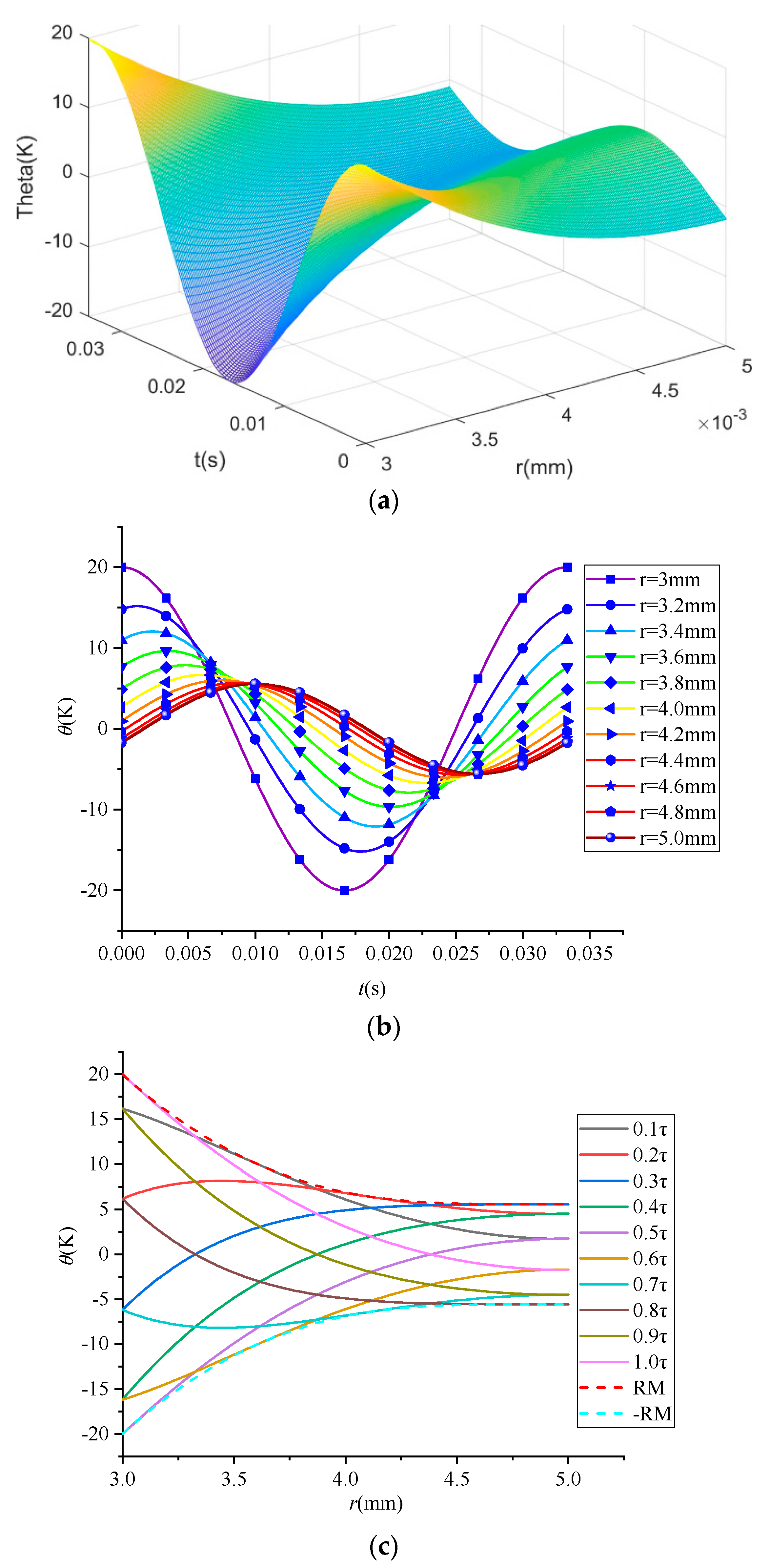
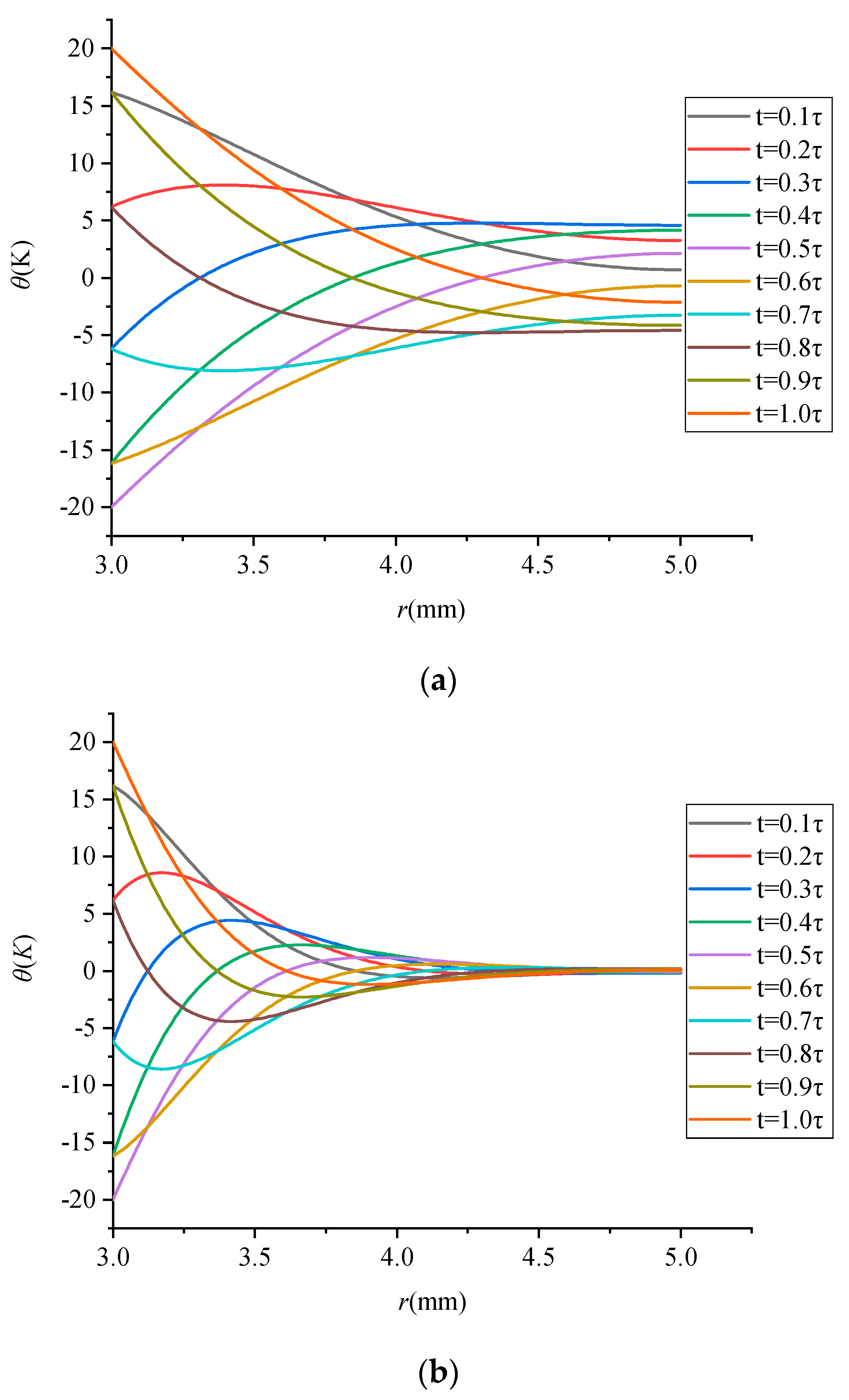
The temperature distribution at different moments calculated by Equation (21) is shown in Figure 5. Initially, the inner diameter r₁ is 3 mm, the outer diameter r₂ is 5 mm, the frequency f is 30 Hz, and the temperature fluctuation amplitude A is 20 K. The results indicate that the temperature distribution in the circular tube changes periodically under the boundary conditions, accompanied by a phase lag, as shown in Figure 5.

Figure 5 shows the amplitude variation curve with time and radius. Figure 5a is a three–dimensional amplitude–time–radius (θ–t–r) panorama of a period. As can be seen from the figure, the curve varies with time and radius in periodic cosine. The amplitude–radius (θ–r) curve and amplitude–time (θ–t) curve are plotted, as shown in Figure 5b and Figure 5c, respectively. Figure 5b shows the amplitude variation with time at different tube thicknesses. It can be seen from the figure that with the increase in the thickness, the amplitude gradually decreases and the phase angle gradually shifts backward. Figure 5c shows the temperature distribution curve within a period τ at different moments. The dotted lines are the envelope line. The figure indicates that the amplitude decreased with the increase in wall thickness.

The temperature distribution curves for aluminum alloy and carbon fiber are shown in Figure 6a,b, respectively. The temperature distribution curves within a period τ at different moments are plotted on the horizontal axis of r₁ ≤ r ≤ r₂.

By comparing the two figures, we can see that the influence of physical property difference on the temperature distribution of the tube made from aluminum alloy is that the temperature distribution in the tube wall thickness is relatively uniform due to the large thermal diffusivity and small change rate of the temperature distribution curve. However, the heat diffusion coefficient of the carbon fiber circular tube is small, the temperature distribution curve change rate is large, the temperature distribution in the tube wall thickness is not uniform, and the temperature of the near–adiabatic part of the outer diameter of the circular tube (4.25 mm–5 mm) basically remains unchanged, and no more heat exchange occurs.

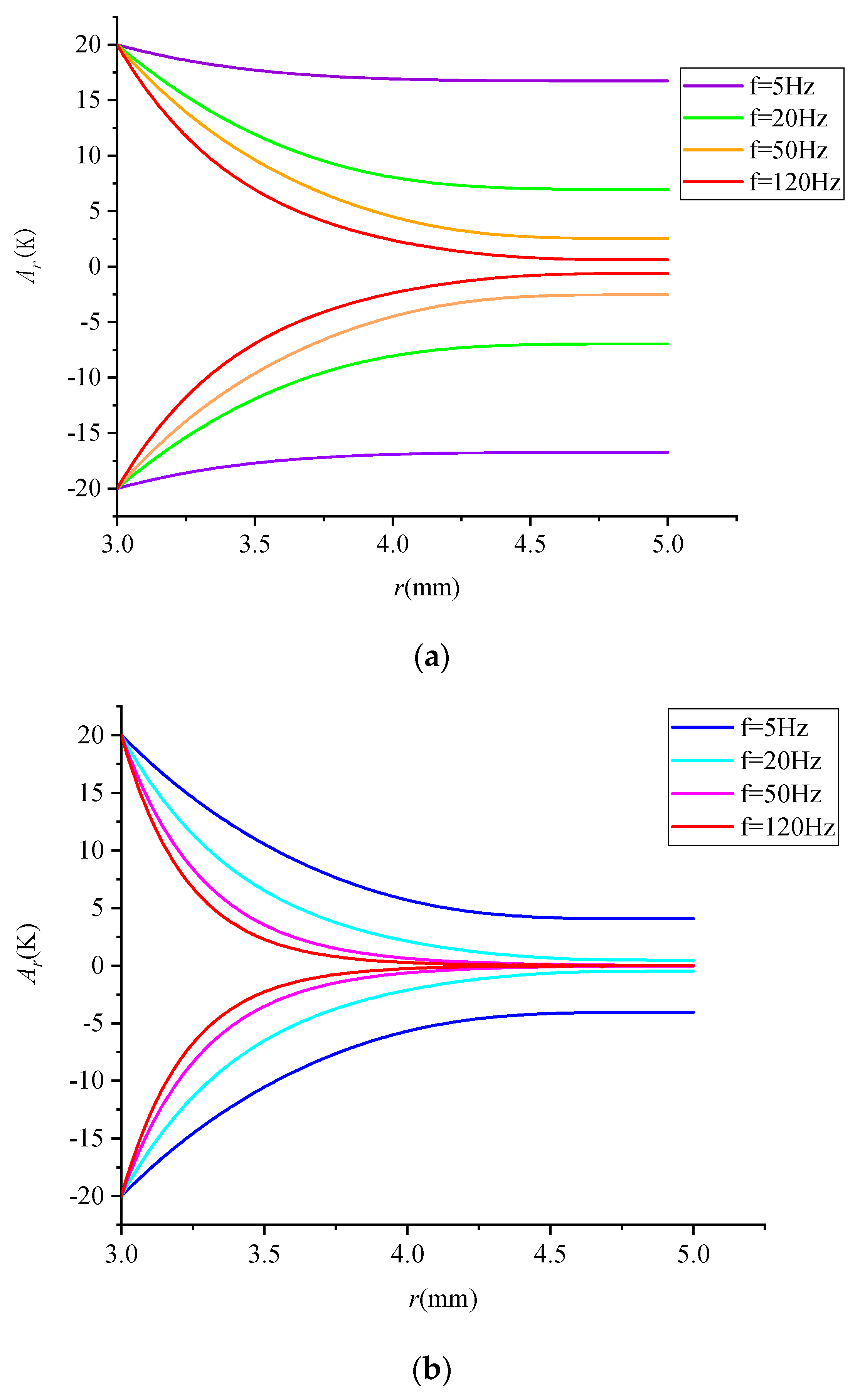
4.1.2. The Influence of Frequency f on Temperature Distribution

The expression of A_r, the temperature distribution amplitude of the regenerator, was obtained according to Equation (22). The change in the temperature distribution amplitude was affected by frequency, as shown in Figure 7. The amplitude distribution curve reflects the heat storage capacity of the regenerator at different frequencies. The smaller the frequency, the stronger the heat storage capacity of the regenerator, and the larger the heat exchange capacity of each cycle, which is also proved by the subsequent calculation of the periodic heat transfer Q_en (Equation (34)). The results also indicate that the temperature distribution became increasingly less uniform with the increase in frequency under the condition of the same tube wall thickness. In terms of circular tubes made from carbon fiber, the temperature at the near–adiabatic part tended to be constant at a frequency of more than 50 Hz, suggesting that no heat exchange occurred at the near–adiabatic part and that such part no longer contributed to heat transfer.

4.1.3. The Influence of Relative Wall Thickness w on Temperature Distribution

h is defined as the tube wall thickness; then:

$$h=r_2-r_1$$

(25)

The attenuation of amplitude has a significant influence on the performance of the regenerator, which is affected by material thermal diffusivity α, working frequency f, and internal and external radius r₁ and r₂, which can be expressed as:

$$w=\frac{h}{{\delta }_k}$$

(26)

Therefore, the dimensionless parameter w is the ratio of the tube wall thickness h to the thermal penetration depth δ_k, which is also known as “relative wall thickness”. It involves all the parameters affecting the change in amplitude and is an important parameter to be discussed later. δ_k is widely used in regenerators and is expressed as [32]:

$${\delta }_k=\sqrt{a/\omega }$$

(27)

If r₂ is assumed to be a constant, then h can be changed by changing r₁*, and the dimensionless h* is defined as:

$$h^{*}=\frac{r_2-{r_1}^{*}}{h}$$

(28)

where r₁ < r₁* < r₂, the dimensionless amplitude $A_h^{*}$ corresponding to the dimensionless wall thickness h* is defined as:

$$A_h^{*}=\frac{A_r({r_1}^{*})}{A}=\left|\frac{(J_1(\sqrt{-i}\beta r_2)Y_0(\sqrt{-i}\beta {r_1}^{*})-Y_1(\sqrt{-i}\beta r_2)J_0(\sqrt{-i}\beta {r_1}^{*}))}{Y_0(\sqrt{-i}\beta r_1)J_1(\sqrt{-i}\beta r_2)-Y_1(\sqrt{-i}\beta r_2)J_0(\sqrt{-i}\beta r_1)}\right|$$

(29)

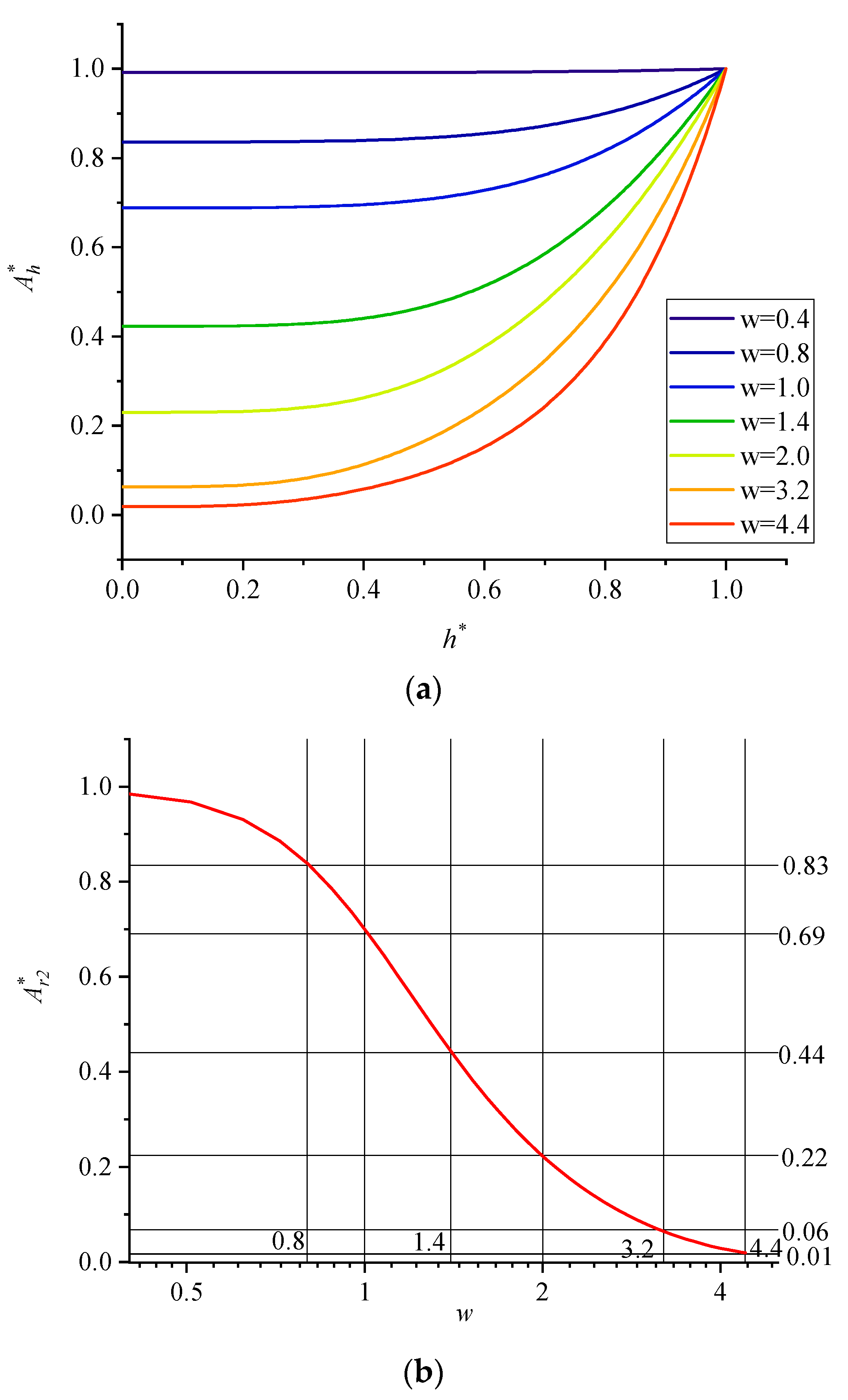
When the relative wall thickness w is 0.4, 0.8, 1.0, 1.4, 2.0, 3.2, and 4.4, the variation rule of dimensionless temperature fluctuation amplitude distribution $A_h^{*}$ along the dimensionless wall thickness h* is shown in Figure 8a. As can be seen from the figure, with the increase in the relative wall thickness w, temperature distribution became less uniform and heat transfer capacity significantly decreased.

Figure 8b shows the variation in the dimensionless temperature fluctuation amplitude $A_{r_2}^{*}$ along the adiabatic boundary with w. It can be calculated by:

$$A_{r_2}^{*}=\left|\frac{(J_1(\sqrt{-i}\beta r_2)Y_0(\sqrt{-i}\beta r_2)-Y_1(\sqrt{-i}\beta r_2)J_0(\sqrt{-i}\beta r_2))}{Y_0(\sqrt{-i}\beta r_1)J_1(\sqrt{-i}\beta r_2)-Y_1(\sqrt{-i}\beta r_2)J_0(\sqrt{-i}\beta r_1)}\right|$$

(30)

In Figure 8b, the horizontal axis is scaled in logarithmic coordinates. The figure shows the variation law of the dimensionless temperature fluctuation amplitude A₀* of the adiabatic wall with the relative wall thickness w, which is analyzed from three perspectives:

First, when 0 < w < 1, $A_{r_2}^{*}$ decreases slowly with the increase in w. Second, when 1 < w < 2, $A_{r_2}^{*}$ decreases rapidly with the increase in w, especially when w = 1.4. Third, when 2 < w < 4.4, $A_{r_2}^{*}$ decreases rapidly with the increase in w, especially after w > 4.4, $A_{r_2}^{*}$ → 0. When the relative wall thickness w = 4.4, the fluctuation range at the center of the tube is close to 0, and the contour lines are, respectively, drawn when $A_{r_2}^{*}$ is equal to 0.83, 0.69, 0.44, 0.22, 0.06 and 0.01.

4.2. Heat Transfer Coefficient of Circular Tube Regenerator under Oscillation

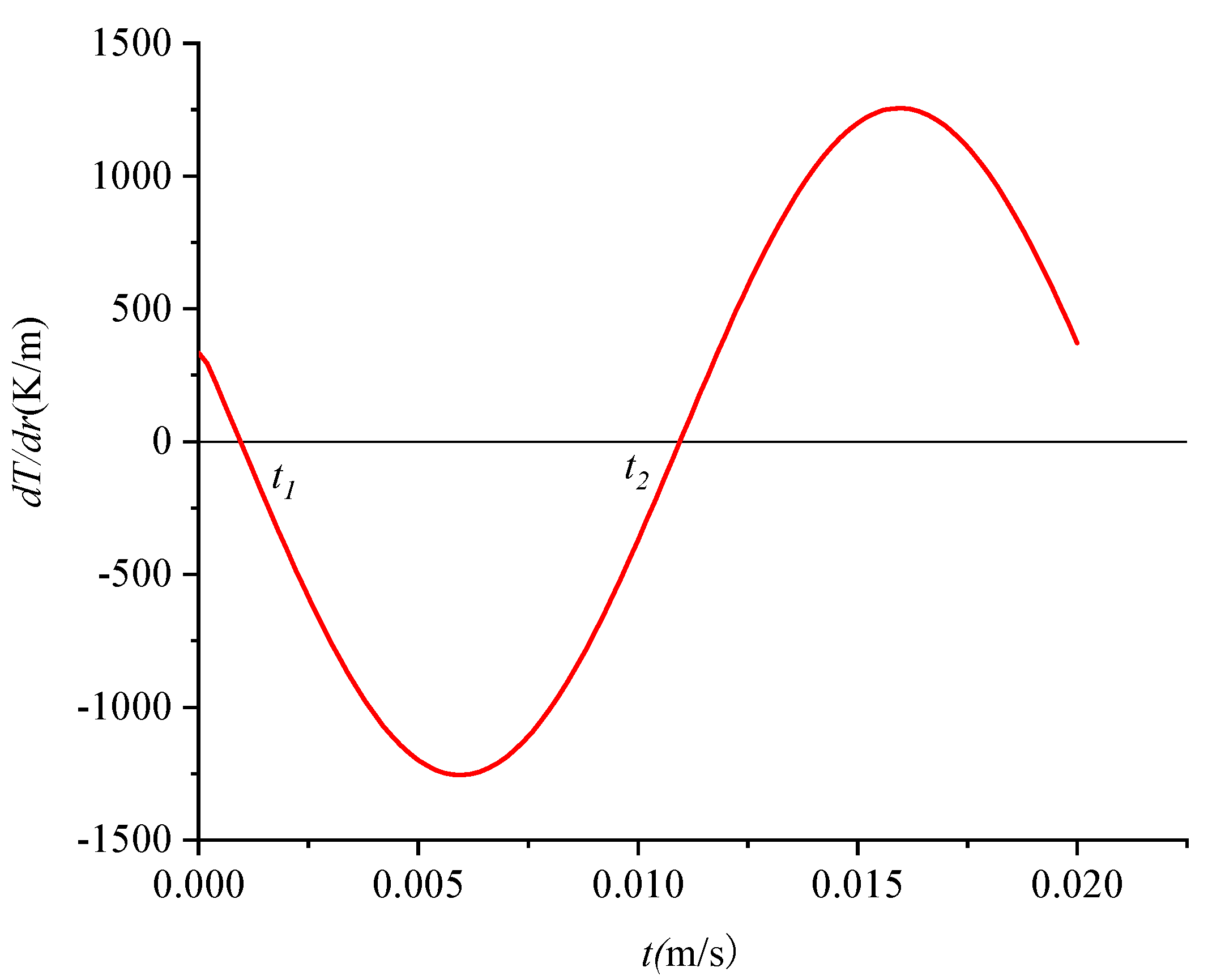
The regenerator periodically stores and releases heat. The heat stored in a period could be calculated by integrating the temperature gradient of the wall surface. According to Equation (20), the temperature gradient equation can be derived as:

$$\frac{\partial T\left(r\right)}{\partial r}=\mathrm{Re}\left[\sqrt{-i}\beta (\frac{A(J_1(-\sqrt{-i}\beta r_2)Y_1(\sqrt{-i}\beta r)+Y_1(\sqrt{-i}\beta r_2)J_1(\sqrt{-i}\beta r))}{Y_0(\sqrt{-i}\beta r_1)J_1(\sqrt{-i}\beta r_2)-Y_1(\sqrt{-i}\beta r_2)J_0(\sqrt{-i}\beta r_1)}){\mathrm{e}}^{i\omega t}\right]$$

(31)

The temperature gradient curve at the inner–wall surface is shown in Figure 9.

In a cycle, the amount of heat absorbed through the inner wall of the tube Q_en is equal to the amount of heat discharged Q_ex; thus, we have:

$$Q_{\tau }=Q_{en}+Q_{ex}=0$$

(32)

In Figure 9, t₁ and t₂ are the heat Q_en releases within a cycle, which could be calculated by integrating the temperature gradient at time [t₁, t₂] and expressed as:

$$Q_{en}=-\lambda S{\displaystyle {\int }_{t_1}^{t_2}{\frac{\partial T(r,\mathrm{t})}{\partial r}|}_{w}dt}$$

(33)

After solving:

$$Q_{en}=\lambda SA\beta \left|\sqrt{-i}\frac{-J_1(\sqrt{-i}\beta r_2)Y_1(\sqrt{-i}\beta r_1)+Y_1(\sqrt{-i}\beta r_2)J_1(\sqrt{-i}\beta r_1)}{Y_0(\sqrt{-i}\beta r_1)J_1(\sqrt{-i}\beta r_2)-Y_1(\sqrt{-i}\beta r_2)J_0(\sqrt{-i}\beta r_1)}\right|\frac{2}{\omega }$$

(34)

where S is the heat transfer area of a single circular tube, which is directly related to the wall thickness h and length l. The total heat exchange time of the Q_en is the period τ, and the temperature difference ∆T = 2A. Therefore, the EHTC K of the circular tube regenerator could be calculated by temperature gradient Equation (31) and heat Equation (34).

$$K=\frac{Q_{en}}{\tau S\mathsf{\Delta }T}=\lambda \beta \left|\sqrt{-i}\frac{-J_1(\sqrt{-i}\beta r_2)Y_1(\sqrt{-i}\beta r_1)+Y_1(\sqrt{-i}\beta r_2)J_1(\sqrt{-i}\beta r_1)}{Y_0(\sqrt{-i}\beta r_1)J_1(\sqrt{-i}\beta r_2)-Y_1(\sqrt{-i}\beta r_2)J_0(\sqrt{-i}\beta r_1)}\right|\frac{1}{2\pi }$$

(35)

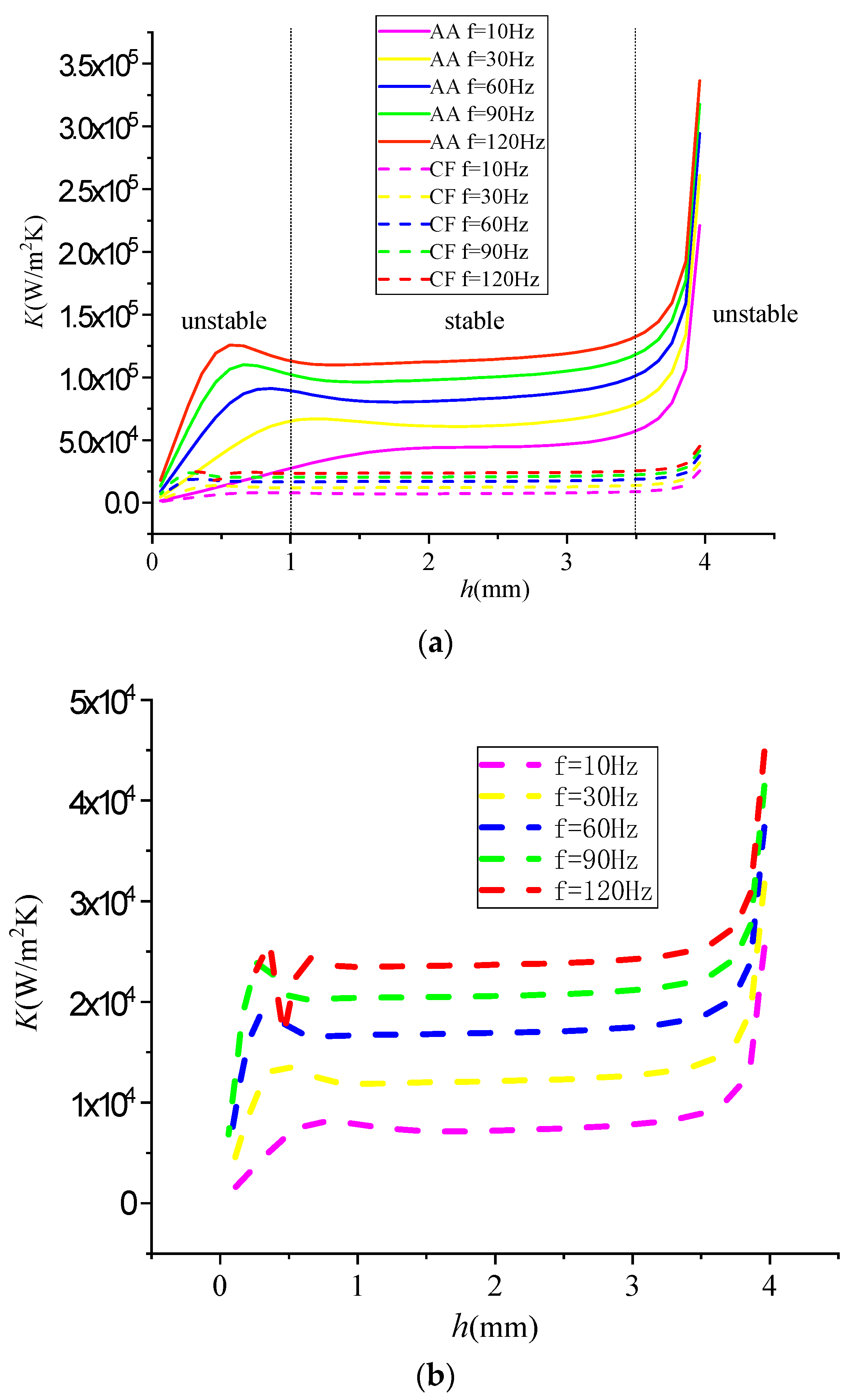
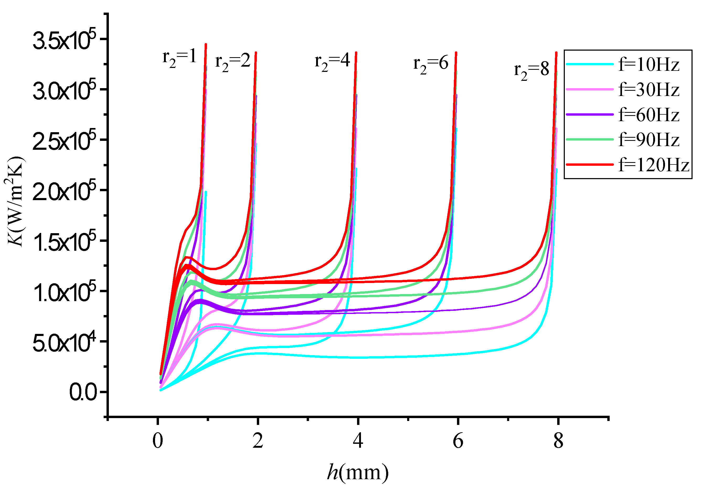
The change in the EHTC K with wall thickness h at different frequencies is shown in Figure 10. According to the structural characteristics of the hexagonal grid tube, the outer diameter r₂ of the equivalent circular tube is assumed to be the ultimate wall thickness. In other words, the wall thickness h changes based on constant r₂, and could be changed by changing r₂.

Figure 10 shows the relationship between the heat transfer coefficient K and the tube wall thickness. It can be known from $h=r_2-r_1$ that h is a function of r₂ and r₁. When r₂ remains unchanged (r₂ = 4 mm for research), the larger r₁ is, the smaller h is and the thinner the tube wall is. As can be seen from Figure 10, at a certain frequency, the heat transfer coefficient increases with the wall thickness when the wall thickness h of circular tube is small (0 < h < 1 mm). In the area where the tube wall is at medium thickness (1 < h < 3.5), the heat transfer coefficient increases slowly and then remains basically stable. When the tube wall thickness h is large (3.5 < h < 4 mm), the heat transfer coefficient approaches infinity. The heat transfer coefficient is unstable when the wall thickness is too large or too small. In addition, it also remains unstable with the change in heat transfer coefficient. The heat transfer coefficient is unstable when the tube wall thickness is larger or smaller, and the heat transfer coefficient is also unstable with the change in heat transfer coefficient. The variation trend of carbon fiber is the same as that of aluminum alloy, except that the heat transfer coefficient of carbon fiber is small, the variation amplitude of the heat transfer coefficient with frequency is relatively small, and the cut–off point of the stability zone is moved forward compared with aluminum alloy. Therefore, the selection of wall thickness is required, and the appropriate wall thickness should avoid the unstable zone at both ends. Due to the large range of the stability zone, taking aluminum alloy as an example, the wall thickness is between 1 < h and < 3.5 mm, so the concept of “limit wall thickness” is introduced to determine the optimal value of wall thickness.

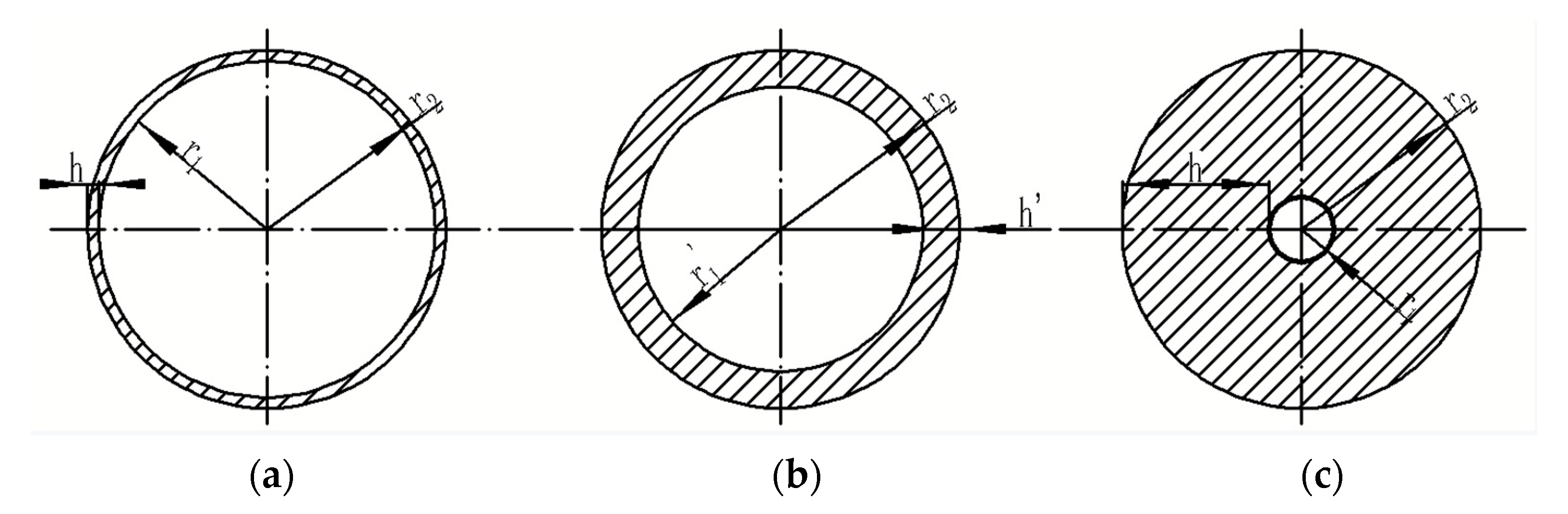
The relationship between the inner–wall thickness and the outer diameter of the tube can be explained from three perspectives. The influence mechanism of the wall thickness of the tube on the heat transfer coefficient is explored in three cases: ultra–thin wall thickness, normal wall thickness, and ultra–thick wall thickness, as shown in Figure 11a–c.

The following conclusions can be drawn from the analysis and numerical verification of Equation (32). First, in the case of ultra–thin wall thickness, when r₁ → r₂, the wall thickness h → 0 and the heat storage volume is V → 0. In the case of ultra–thin wall thickness, the heat storage Q_en → 0 in a cycle and the EHTC is sharply reduced, approaching 0, K → 0, which is an unstable condition of the failure of the heat storage capacity. Second, if the wall is ultra–thick when the inner diameter of the circular tube r₁ → 0, the heat exchange area S → 0, resulting in the EHTC K → +∞, and the heat exchange capacity of the regenerator is reduced, an unstable working condition in which the EHTC could only meet the heat exchange requirements when it becomes infinite. Therefore, the practical conditions of ultra–thin wall thickness and ultra–thick wall thickness should be avoided. In the case of normal wall thickness (1 mm < r₁ < 3.5 mm), the heat transfer coefficient remains basically unchanged with the change in wall thickness, but is positively correlated with the frequency, which conforms to the heat transfer theory. Therefore, it should be selected in practical applications, as shown in Figure 10.

The above analysis brings about an interesting and critical question, which is the choice of ultimate wall thickness r₂. The heat transfer coefficients when the ultimate wall thickness r₂ is 1, 2, 4, 6 and 8 mm are shown in Figure 12; the heat transfer coefficient increases with the increase in wall thickness h. When r₂ = 1, in the “narrow” wall thickness, the heat transfer coefficient basically has no stable region, and its value varies from zero to infinity. However, when taking the other values of r₂ > 1, the K value is stable in a certain area, and the sizes of the stable areas are basically the same; first it goes up, then it goes down, and then it goes to infinity. Therefore, the increase in wall thickness is not beneficial for the increase in K value. So, in the value of the limited wall thickness r₂, we avoid the narrow area ($r_2\ne 1$) and consider the full use of materials at the same time, so the limited wall thickness should not be large. This is the purpose of the concept of “ultimate wall thickness”. Combined with the requirements of the thermal penetration depth of the material, the ultimate wall thickness r₂ is 2 mm in this case. According to Figure 10 and Figure 12, it can be determined that there is an optimal value of h and r₂.

4.3. Optimization of Tube Thickness Considering Specific Surface Area

It would be a key task to determine the wall thickness and inner diameter of a circular tube in the design process. Theoretically, heat transfer area is independent of heat transfer coefficient, but some constraints need to be considered in practical applications. The size of the regenerator cannot be arbitrarily large, so it is of practical significance to explore heat transfer process under the constraints of a given regenerator volume. The constraints can be described by specific surface area, the ratio of the surface area of the inner circle to the tube volume. The calculation results are:

$$\frac{A_s}{V}=\frac{2\pi r_1}{\pi ({r_2}^2-{r_1}^2)}=\frac{2r_1}{(2r_1+h)h}$$

(36)

Therefore, the product of heat transfer coefficient and specific surface area was selected as the target parameter to determine the optimal size of the circular tube in this paper. It is called specific volume heat transfer capacity, denoted as K_v, and can be calculated by:

$$K_v=K\frac{A_s}{V}=\frac{\lambda \beta }{\pi }\left|\sqrt{-i}\frac{-J_1(\sqrt{-i}\beta r_2)Y_1(\sqrt{-i}\beta r_1)+Y_1(\sqrt{-i}\beta r_2)J_1(\sqrt{-i}\beta r_1)}{Y_0(\sqrt{-i}\beta r_1)J_1(\sqrt{-i}\beta r_2)-Y_1(\sqrt{-i}\beta r_2)J_0(\sqrt{-i}\beta r_1)}\right|\frac{r_1}{(2r_1+h)h}$$

(37)

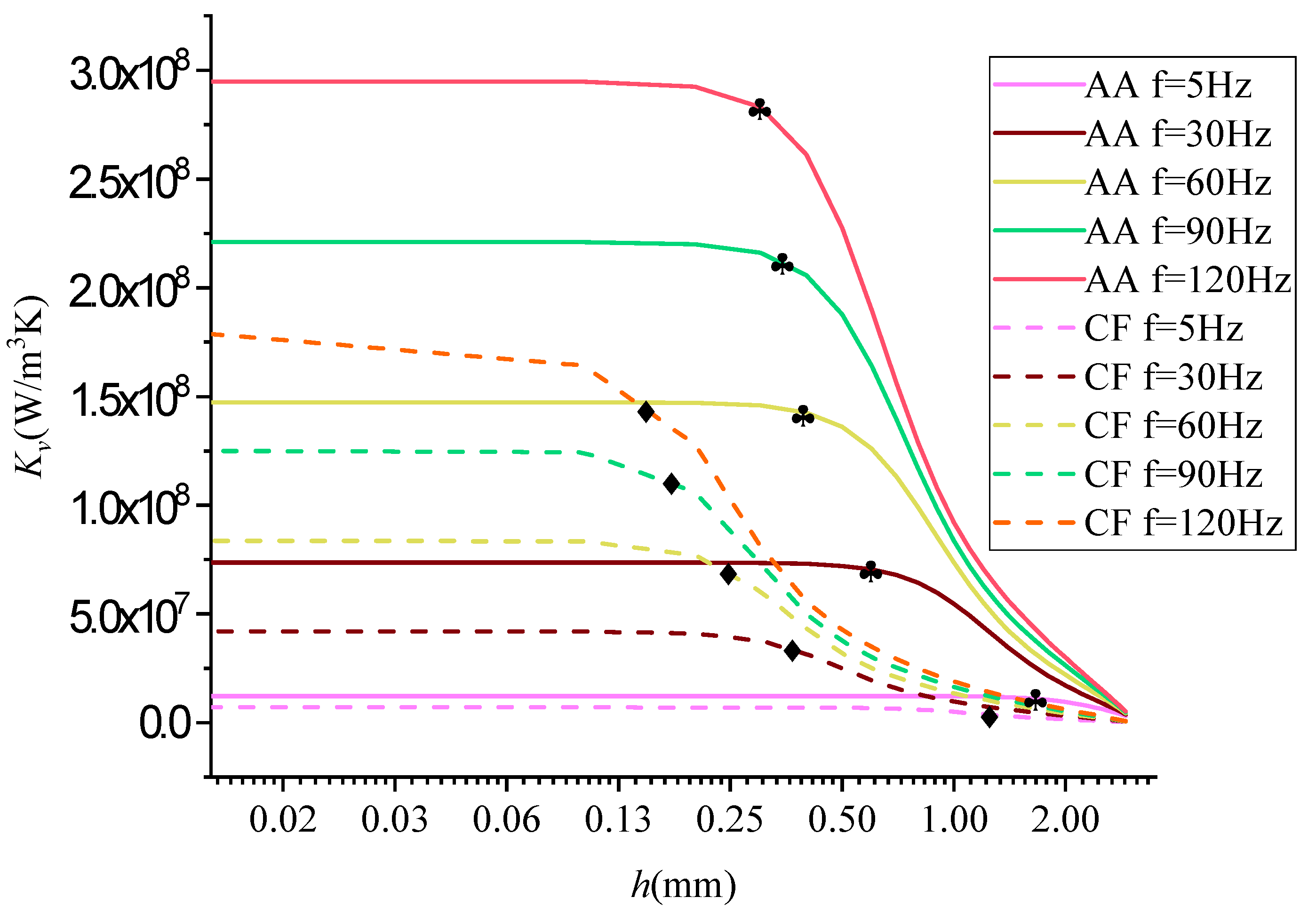
This parameter actually reflects the relationship between the overall heat exchange performance of the regenerator and the wall thickness h and the frequency f, as shown in Figure 13.

It can be found that K_v decreased monotonically with the wall thickness h, indicating that the larger the specific surface area, the better the overall heat transfer performance. At the same time, when the wall thickness was small enough, the overall heat transfer performance was stable, reaching its optimum. Therefore, the heat exchange performance was not significantly changed by further increasing specific surface area, implying that there is an optimal wall thickness. If the wall thickness exceeded its optimal value, specific surface area would increase, and flow resistance would also rapidly increase, which could not improve the overall efficiency of the Stirling machine.

Take aluminum alloy as an example; when the frequency f = 30 Hz, the corresponding thickness h = 1 mm, and when f > 30 Hz, h was between 0.5 and 1 mm. This conclusion verifies the relationship between the heat transfer coefficient K and the wall thickness h in Figure 10. As can be seen from Figure 13, the SVHTC of the aluminum alloy was greater than that of carbon flux, and the difference between the two increased with frequency. The optimal wall thickness of tube made from aluminum alloy should not exceed the “♣” number marked in the figure. Before “♣” number, the SVHTC K_v was at a high level and then decreased slowly with the increase in the wall thickness h. After “♣” number, the SVHTC K_v decreased rapidly with the increase in the wall thickness h until it approached 0. The optimal wall thickness h of the tube made from carbon fiber should not exceed the mark “♦” in the figure, and its forward and backward variation trend was the same as that of the aluminum alloy. The SVHTC K_v of the same material increased with the increase in frequency f. Compared with the aluminum alloy, the SVTHC of carbon fiber decreased with the increase in frequency. Take aluminum alloy as an example; when the frequency f = 30 Hz, the corresponding thickness h = 1 mm, and when f > 30 Hz, h was between 0.5 and 1 mm. This conclusion verifies the relationship between the heat transfer coefficient K and the wall thickness h in Figure 10.

When the regenerator was made of aluminum alloy, the outer diameter r₂ was 2.5 mm, the inner diameter r₁ was 1.5 mm, the thickness h was 1 mm, the working frequency f was 20 Hz, the heat transfer capacity K_v was 2 × 10⁷ W/m³K, the heat transfer difference ∆T was 1 K, the porosity of the regenerator was 0.46, and the total volume V_r was 65.2 cm³; then, the heat exchange of the regenerator was calculated by:

$$q_r=K_v{V}_r\mathsf{\Delta }T=1.34\mathrm{kW}$$

(38)

It reached the magnitude of kW, as Equation (38) shows; when $\mathsf{\Delta }T=1\mathrm{K}$ and $V_r=1{\mathrm{cm}}^3$, the heat transfer was numerically equal to Kv. The higher the frequency, the greater the heat change. Under such working conditions, the heat exchange performance of the regenerator is undoubtedly satisfactory.

According to the research results of this paper, some suggestions are put forward for the design of a Stirling machine regenerator: Firstly, according to Figure 8b, the relative thickness w was set at about 0.8 and w < 1, making the heat storage material basically in the state of thermal permeability. Secondly, according to Equation (34) for heat exchange, thermal diffusivity α and working frequency f of several materials were comprehensively considered. Thirdly, the ultimate wall thickness r₂ and h were selected according to the analysis results in Figure 12 to obtain the inner diameter r₁ further. At this point, the parameters of HTGR were primarily determined. Then, the working point of h was verified, as displayed in Figure 13. If K_v is at a high level and locates in the slow decline area at the beginning stage, the optimization design is completed. If K_v does not meet the requirement, then one should return to the second step, which means continuing to search for the optimal design by jointly considering the thermal spreading coefficient of the material and working frequency.

4.4. Verifying the Analytical Solution

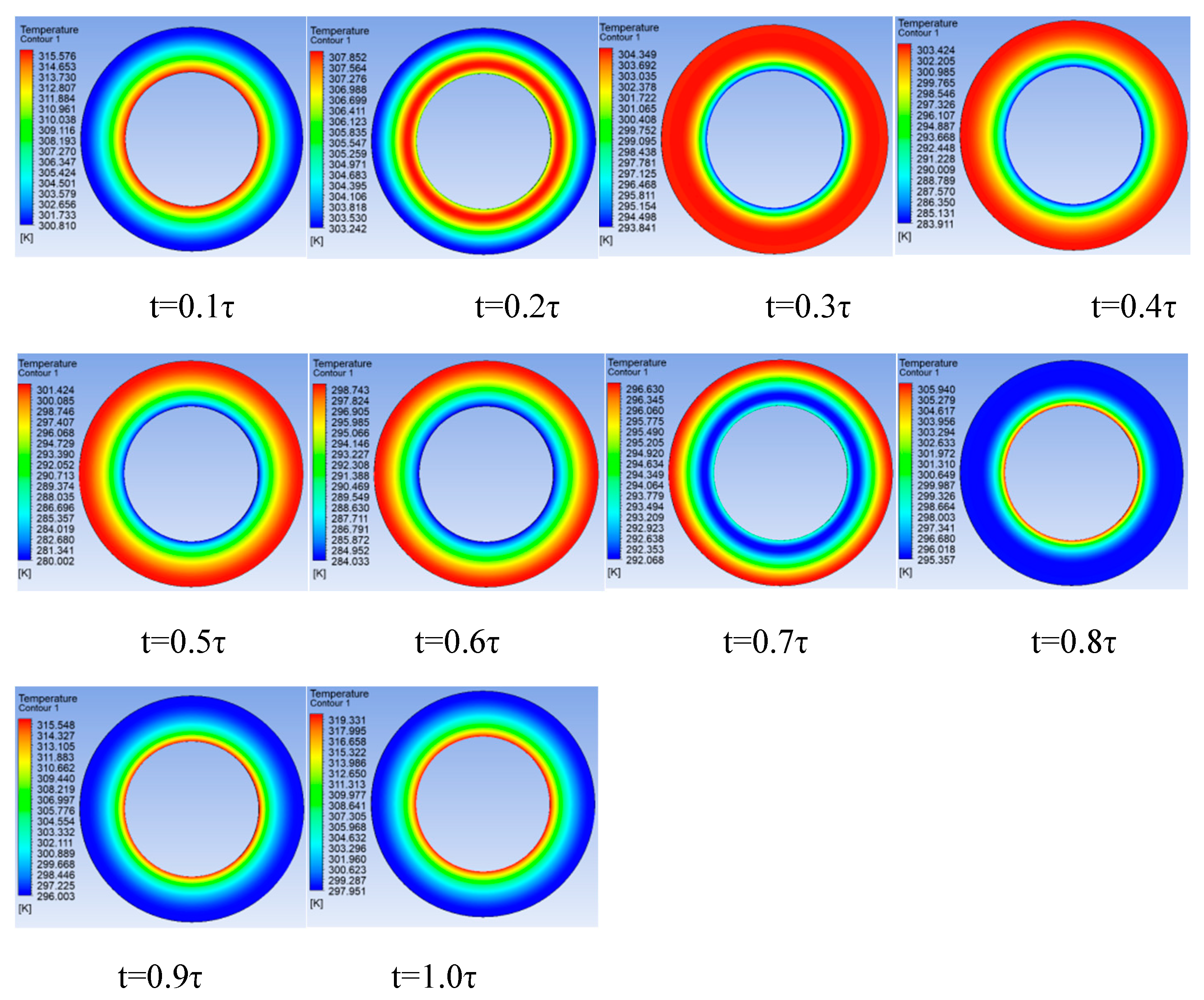
The circular tube model was established, and the outer diameter of the circular tube was r₁ = 3 mm and r₂ = 5 mm, respectively. The numerical simulation was carried out using Fluent software. 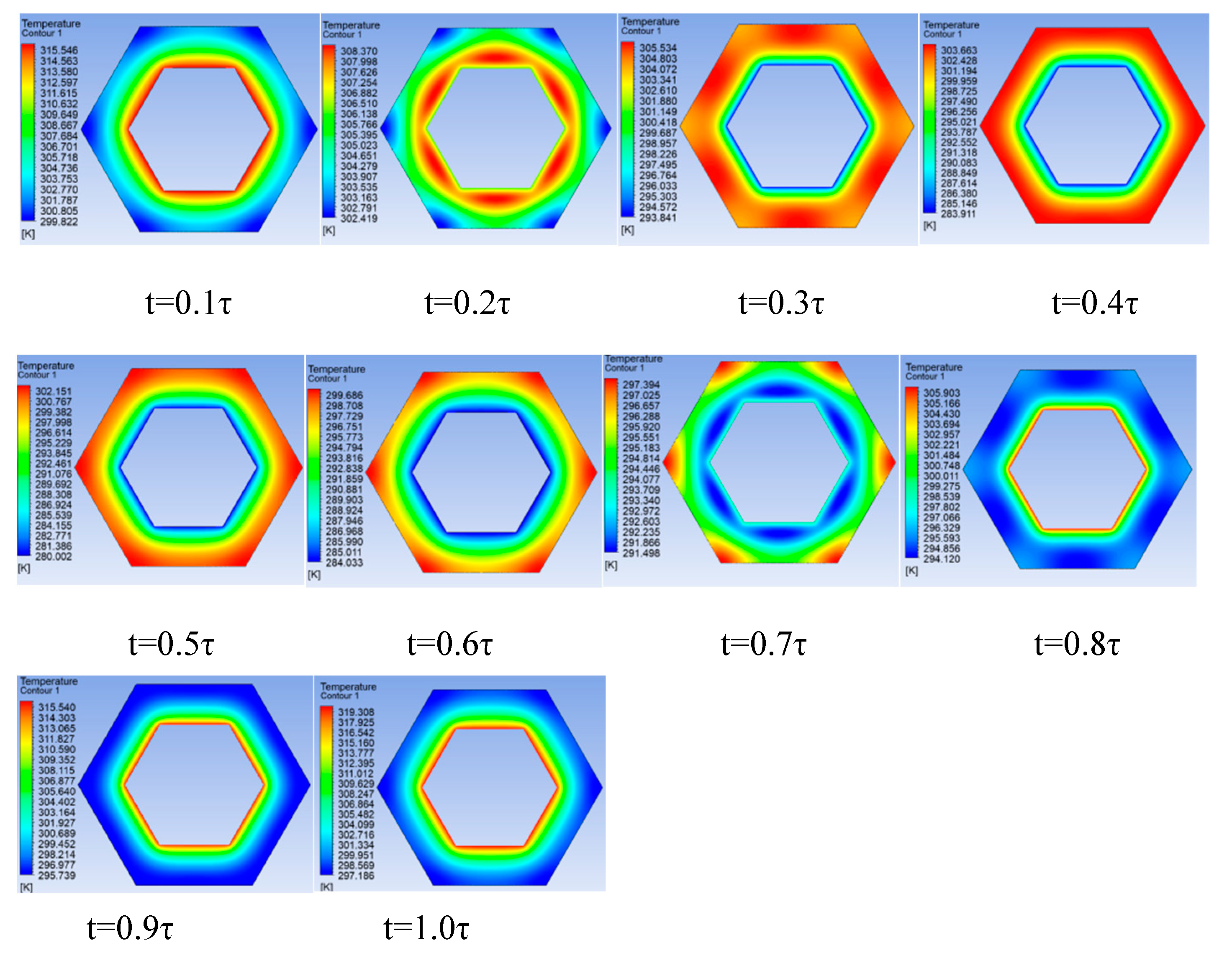The inner–wall temperature changed periodically: $T=20\sin \left(2\pi ft\right)$, the outer wall was an adiabatic boundary; a transient model, first–order upwind difference scheme and SIMPLE algorithm were adopted; the convergence condition of the energy equation was that the residual was less than $e^{-9}$; so, the temperature cloud diagram of the circular tube at a time τ was obtained, as shown in Figure 14. Through the cloud image, the process of heat absorption and emission through the wall of the circular tube regenerator can be clearly seen.

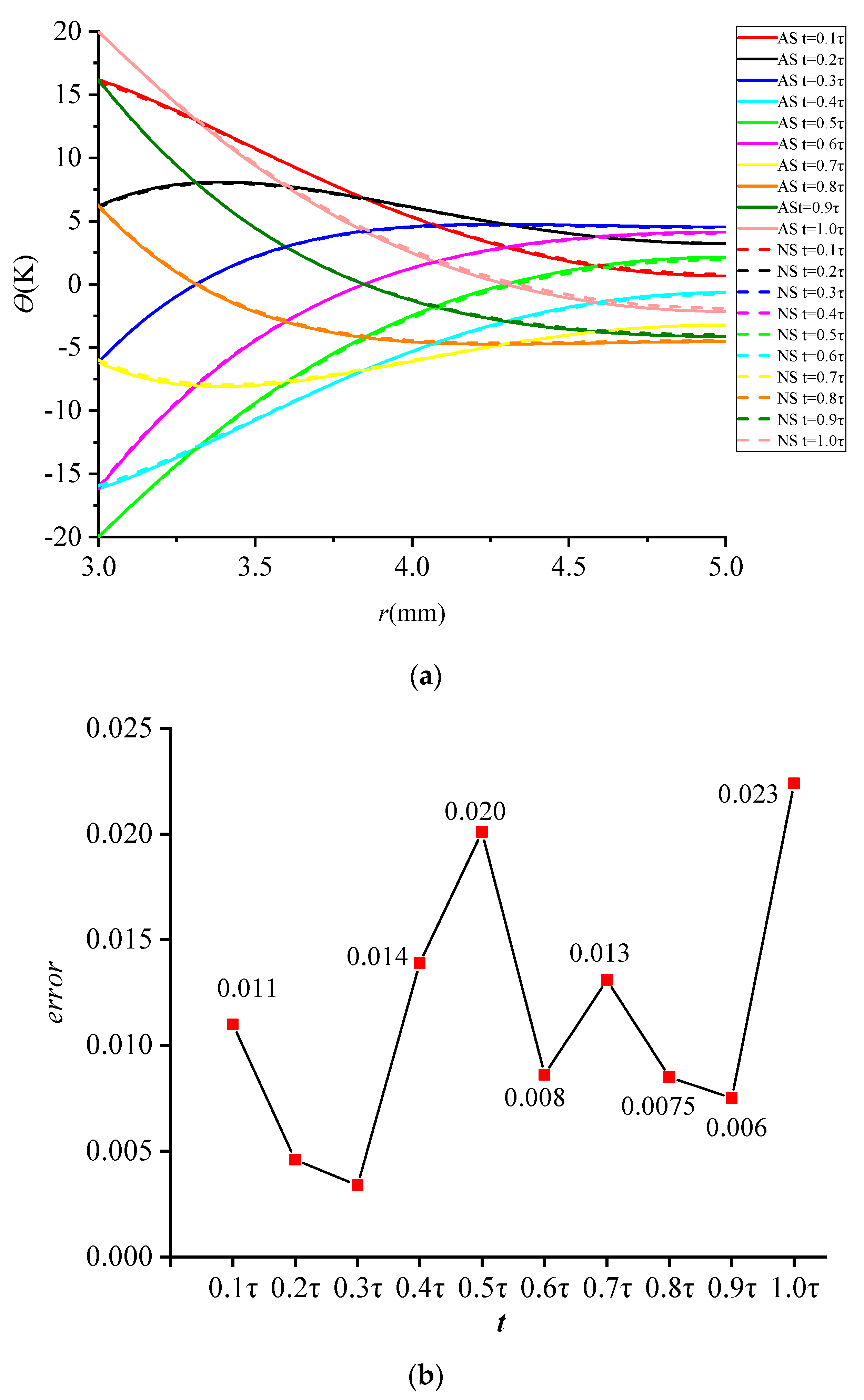
The numerical solution was compared with the analytical solution, and the result is shown in Figure 15.

In Figure 15a, the solid line is the analytical solution and the dashed line is the numerical solution. The two curves are in good agreement, which directly verifies the correctness of the analytical method for the circular tube regenerator. Figure 15b shows the degree of difference between the two curves. The maximum mean square error is not more than 2.3%.

The model of a regular hexagonal tube was established in the same way, according to the equivalent relation with the circular tube; the regular hexagon tube edge a = 3.14 mm and b = 5.24 mm. The temperature cloud diagram of the regular hexagonal tube at a time τ was obtained, as shown in Figure 16. The process of heat absorption and emission through the regular hexagonal tube wall in a period τ can be clearly seen through the cloud image.

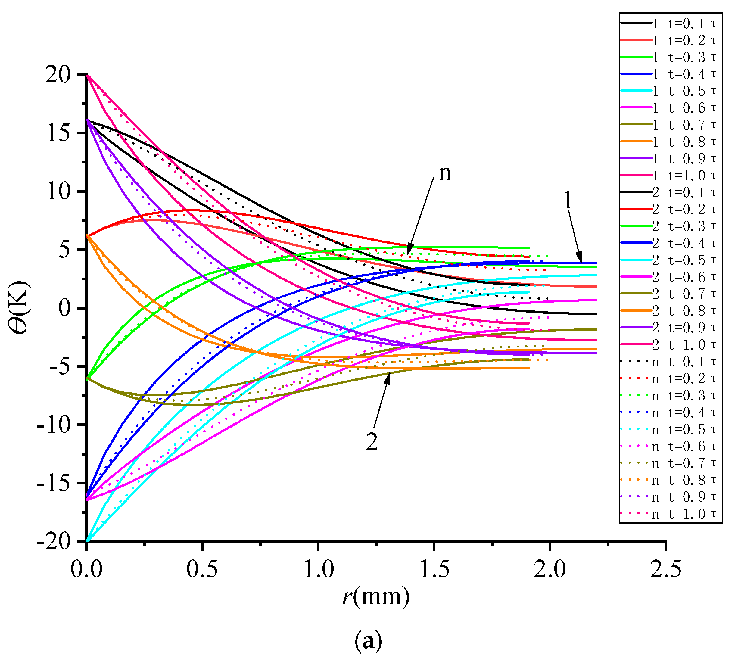
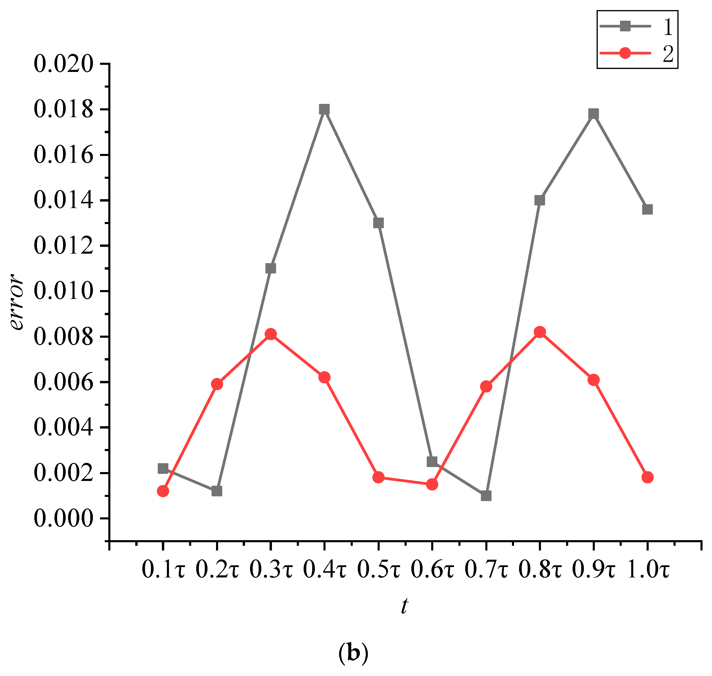
The numerical solution of the regular hexagon tube was compared with that of the circular tube. The result is shown in Figure 17a, where 1 and 2 are the two endpoints of the regular hexagon (Figure 2b); the dashed line stands for the numerical solution of the circular tube. The error between the end points 1 and 2 of the regular hexagonal tube and the circular tube is shown in Figure 17b.

5. Conclusions

In this paper, based on the two basic conditions of equal heat exchange area and equal heat storage, the geometric space of a regular hexagonal tube was equivalently transformed into a circular tube, and the HTGR was proved to be suitable for a inverse Stirling cycle at room temperature through theoretical analysis. Taking aluminum alloy and carbon fiber as examples, this paper provided a reference case for the design and operation of a regenerator at room temperature. The analytical expression of the Bessel function for temperature distribution was derived and the heat transfer coefficient of the HTGR was obtained. Two dimensionless parameters affecting the heat transfer mechanism of the HTGR were proposed: one is the relative thickness w, which is composed of four factors: operating frequency f, wall thickness h, ultimate wall thickness r₂, and thermal diffusivity α; and the other is the SVHTC K_v of the specific surface area, which reflects the overall heat transfer performance of the regenerator. The conclusions of this paper are summarized as follows:

• Based on the influence of wall thickness on the heat transfer coefficient, the heat transfer mechanism of the HTGR was explored. When the heat transfer coefficient of the tube was ultra–thin or ultra–thick, the EHTC decreased sharply or increased infinitely, leading to the failure of the regenerator to store or exchange heat due to functional failure or a loss of heat transfer capacity. Therefore, it is necessary to avoid two unstable areas and select normal wall thickness in the selection of wall thickness. In the stable area, the EHTC could reach 10⁴–10⁵ W/m²·K, indicating that HTGR exhibits excellent heat transfer capacity.
• With the increase in specific surface area, the SVHTC increased, but there was a limit value. When the specific surface area was large enough, the SVHTC was in the high position, and the wall thickness of the grid was optimal at this moment. The relative thickness w was about 0.8, which is the appropriate boundary for heat penetration.
• The limited wall thickness was selected mainly to ensure that the regenerator had a stable heat exchange working area. In the stable working region, the heat transfer coefficient remained constant with the increase in the limited wall thickness, so the appropriate limited wall thickness is very important. When the limited wall thickness was too small, heat transferred quickly through, the heat transfer coefficient was unstable; with the increase in the limited wall thickness, the stable working area became longer and the heat transfer coefficient did not increase. So, an appropriate value can not only ensure sufficient heat exchange but also save materials.
• The frequency had a positive influence on heat transfer performance. With the increase in frequency, the heat exchange performance increased monotonically, so high–frequency operation is beneficial to improve the heat transfer performance of the regenerator.
• The numerical solution of the circular tube was in good agreement with the analytical solution, and the error was less than 2.3%, which indicates the correctness of solving the HTGR with the analytical model. The approximate numerical solution of the regular hexagon tube and the circular tube verifies that the regular hexagon can be transformed into a circle with an error less than 1.8%. In the next step, the heat exchange of a regular hexagonal pipe and circular pipe can be solved to further verify the equivalence of the two structures.

6. Patent

Chinese invention patent “Air Conditioning Temperature Zone Layered Honeycomb Structure with Variable Porosity Regenerator” was invented with the authorization number “ZL202110300042.7”.