Review

Optimization-Based High-Frequency Circuit Miniaturization through Implicit and Explicit Constraint Handling: Recent Advances

by
Anna Pietrenko-Dabrowska
1,2,*,
Slawomir Koziel
2,1 and
Marzieh Mahrokh
2
1
Faculty of Electronics, Telecommunications and Informatics, Gdansk University of Technology, 80-233 Gdansk, Poland
2
Engineering Optimization & Modeling Center, Reykjavik University, 102 Reykjavik, Iceland
*
Author to whom correspondence should be addressed.
Energies 2022, 15(19), 6955; https://doi.org/10.3390/en15196955
Submission received: 14 July 2022 / Revised: 14 September 2022 / Accepted: 15 September 2022 / Published: 22 September 2022

Abstract

:
Miniaturization trends in high-frequency electronics have led to accommodation challenges in the integration of the corresponding components. Size reduction thereof has become a practical necessity. At the same time, the increasing performance demands imposed on electronic systems remain in conflict with component miniaturization. On the practical side, the challenges related to handling design constraints are aggravated by the high cost of system evaluation, normally requiring full-wave electromagnetic (EM) analysis. Some of these issues can be alleviated by implicit constraint handling using the penalty function approach. Yet, its performance depends on the arrangement of the penalty factors, necessitating a costly trial-and-error procedure to identify their optimum setup. A workaround is offered by the recently proposed algorithms with automatic adaptation of the penalty factors using different adjustment schemes. However, these intricate strategies require a continuous problem-dependent adaptation of the penalty function throughout the entire optimization process. Alternative methodologies have been proposed by taking an explicit approach to handle the inequality constraints, along with correction-based control over equality conditions, the combination of which proves to be demonstrably competitive for some miniaturization tasks. Nevertheless, optimization-based miniaturization, whether using implicit or explicit constraint handling, remains a computationally expensive task. A reliable way of reducing the aforementioned costs is the incorporation of multi-resolution EM fidelity models into the miniaturization procedure. Therein, the principal operation is based on the simultaneous monitoring of factors such as quality of the constraint satisfaction, as well as algorithm convergence status. This paper provides an overview of the abovementioned size-reduction algorithms, in which theoretical considerations are illustrated using a number of antenna and microwave circuit case studies.

1. Introduction

The emerging system integration technologies, resulting from the miniaturization trends in contemporary electronic systems, have led to size restrictions on the comprising components, in applications such as integrated system-on-chip (SoP) wireless communication modules, internet of things (IoT), or integrated passive components [1] in RF ICs. Some of the essential passive components occupying considerable space in these systems include microstrip filters [2], capacitors/inductors [3], couplers/dividers [4], and antenna arrays [5]. Various alterations in conventional structures have been proposed to minimize their footprints. These are typically based on the techniques incorporating electromagnetic wave theory along with additional degrees of freedom provided by topological modifications. Some of the popular methods include the use of metamaterial-based (MTM) composite left/right-handed transmission line (CLRH-TL) structures [6,7,8] the employment of artificial transmission lines (ATL) [9,10] the incorporation of half-mode evanescent-mode cavity resonators [11,12] or the introduction of differential bridged-T coils [13,14]. The scope of this work is an optimization-based size reduction in high-frequency devices and not topology adjustment aimed at footprint reduction. Notwithstanding, the frameworks discussed hereinafter may be applied for parameter tuning of antenna and microwave structures designed with the use of the aforementioned (as well as other) topological modifications.
Although the abovementioned techniques ensure reliability in producing reduced-size structures, they contribute to the design complexity both at the conceptual development stage and the subsequent handling of additional geometry parameters. Identification of the optimal design in the sense of resolving the conflict between miniaturization and satisfaction of the design constraints imposed on electrical characteristics can be dealt with through local parameter tuning [15,16,17,18,19,20,21,22,23,24,25,26,27] (in particular, through genuine multi-objective design [28,29,30]), or global search methods [31,32,33]. Still, there are only a few works on optimization-related miniaturization of antenna and microwave structures: some examples can be found in [34,35,36,37,38]. Nevertheless, in these approaches, an optimization algorithm of choice (e.g., firefly optimizer [34] or genetic algorithm [35]) is employed in the last stage of the design process for parameter tuning of geometry parameters aimed at obtaining the required electrical properties of the component under design rather than size reduction. Furthermore, no constraint on the component size is imposed in the optimization procedure, so, in some cases, the footprint of the optimized structure may be actually larger than that of the initial non-optimal design. Regardless of the specific optimization technique, handling of the design constraints tends to be impeded by algorithmic complexity as well as costly and repetitive system evaluations involved in the process. The penalty function approach [39] offers the alleviation of these issues by providing an implicit way of controlling the constraints. Nevertheless, the performance of this approach is strongly based upon the setup of the penalty factors, conventionally adjusted through laborious guesswork and repeated trials. The recently proposed automatic adaptation of the penalty function [40,41] attempts to mitigate this problem by eliminating the trial-and-error stage. Therein, the penalty factors are continuously adjusted based on a concept of sufficient constraint violation improvement for single and multiple design constraints. The automated procedure exercises precise control over the design constraints thereby allowing to obtain competitive miniaturization rates. Yet, another adaptation scheme has been reported in [42], where a continuous observation of a properly quantified combination of the convergence status, and the constraint violation levels has been carried out throughout the entire optimization process. The resulting miniaturization rates are comparable to those obtained using the optimum arrangement of the penalty factors. At the same time, a precise control over the design constraints was achieved.
The abovementioned strategies have been successful in resolving the conflict between miniaturized size and satisfactory system performance levels. However, algorithmic complexities arise due to the multiplicity of the adjustment rules that require continuous monitoring of the optimization procedure. Moreover, the entire adjustment procedure is problem-dependent and needs to be readjusted accordingly. A workaround has been proposed by implementing an explicit method of handling constraints [43,44] using the trust-region (TR) framework as the optimization engine. Therein, the TR search radius is adjusted based on a cheap linear approximation of the design constraints rather than based on the quality of the objective function. This results in a virtual elimination of the challenge of the problem-dependent penalty function adjustment as compared to the implicit approach.
An alternative methodology has been developed as well, based on a separate treatment of equality and inequality constraints [45]. The specific geometry of the feasible regions corresponding to equality constraints (i.e., being thin sets in a set-theory sense) calls for a special treatment to control the design quality in a satisfactory manner. Consequently, in the technique of [45], the equality constraints are treated using a correction-based scheme launched before each iteration of the core algorithm, whereas the inequality constraints are dealt with implicitly using the previously mentioned penalty function approach.
Regardless of the constraint handling approach (in particular, implicit or explicit), optimization-based miniaturization tends to remain a highly expensive task in terms of both computational time and resources. The employment of variable-fidelity EM models [46] has proved to be efficient in reducing the aforementioned costs. The operation of the scheme considered in [46] exploits meticulously defined performance indicators including the quality of the constraint satisfaction, as well as the convergence status of the algorithm. This allows for the precise control of the constraints as well as obtaining satisfactory miniaturization rates at a reduced cost.
This paper provides a review of the aforementioned recent advancements in optimization-based miniaturization of high-frequency components. In particular, we discuss both the implicit and explicit approaches, along with the relevant algorithmic strategies, including acceleration methods. Our considerations are illustrated using a number of specific case studies, including both antenna and microwave passive structures. Recommendations concerning the investigated algorithms are also given. The authors believe that this work may be useful for those readers interested in EM-driven design, automation of size-reduction procedures of high-frequency systems, but also improving their computational efficiency.

2. Optimization-Based Size Reduction

This section recalls a formulation of the optimization-based high-frequency circuit miniaturization task. The relevant recent algorithmic developments will be discussed in subsequent sections: the adaptive penalty function approach in Section 3, explicit constraint handling in Section 4 separate treatment of equality and inequality constraints in Section 5, and multi-resolution adaptive penalty functions in Section 6.
The involved interrelationships between geometrical dimensions and the electrical and field properties of high-frequency structures make their size reduction a challenging problem. This is especially pertinent to miniaturized components, in which topological alterations have been introduced to reduce their footprint (e.g., [47,48,49,50,51,52]). Although these properties may vary to some extent depending on the nature and applications of the specific structure, they are normally evaluated using EM simulations of the corresponding structural dimensions. The latter are expressed as a vector x = [x1 … xn]T, containing n independently adjustable geometry parameters of the structure. It should be emphasized that all of the algorithmic frameworks discussed in this work are generic in the sense that they may utilize any simulation software package selected according to the designer’s preference. In the presented examples, CST Microwave studio has been employed for evaluating high-frequency verification structures, yet, the considered frameworks may also employ, e.g., Ansys HFSS, Sonnet em or dedicated solvers.
The simulation-based high-frequency size reduction problem can be formulated as
x * = arg min x X f A ( x )
where A(x) is the size of the structure (e.g., a footprint area for planar circuits), x* is the optimum design to be found, whereas Xf is the feasible space. The latter contains parameter vectors for which all design constraints are satisfied, which may be of inequality or equality type. Formally, the equality constraints are written as
Seq,k(x) = 0, k = 1, …, neq
and inequality ones as
Sineq,k(x) ≤ sj, k = 1, …, nineq
Thus, the total number of constraints is nc = neq + nineq. A practical issue is that the constraints, apart from the strictly geometric ones, are expensive, as their evaluation requires EM analysis. Here, are a few examples (below, Skl(x, f) denotes the scattering parameter of a considered device for ports k and l at the design x and frequency f):
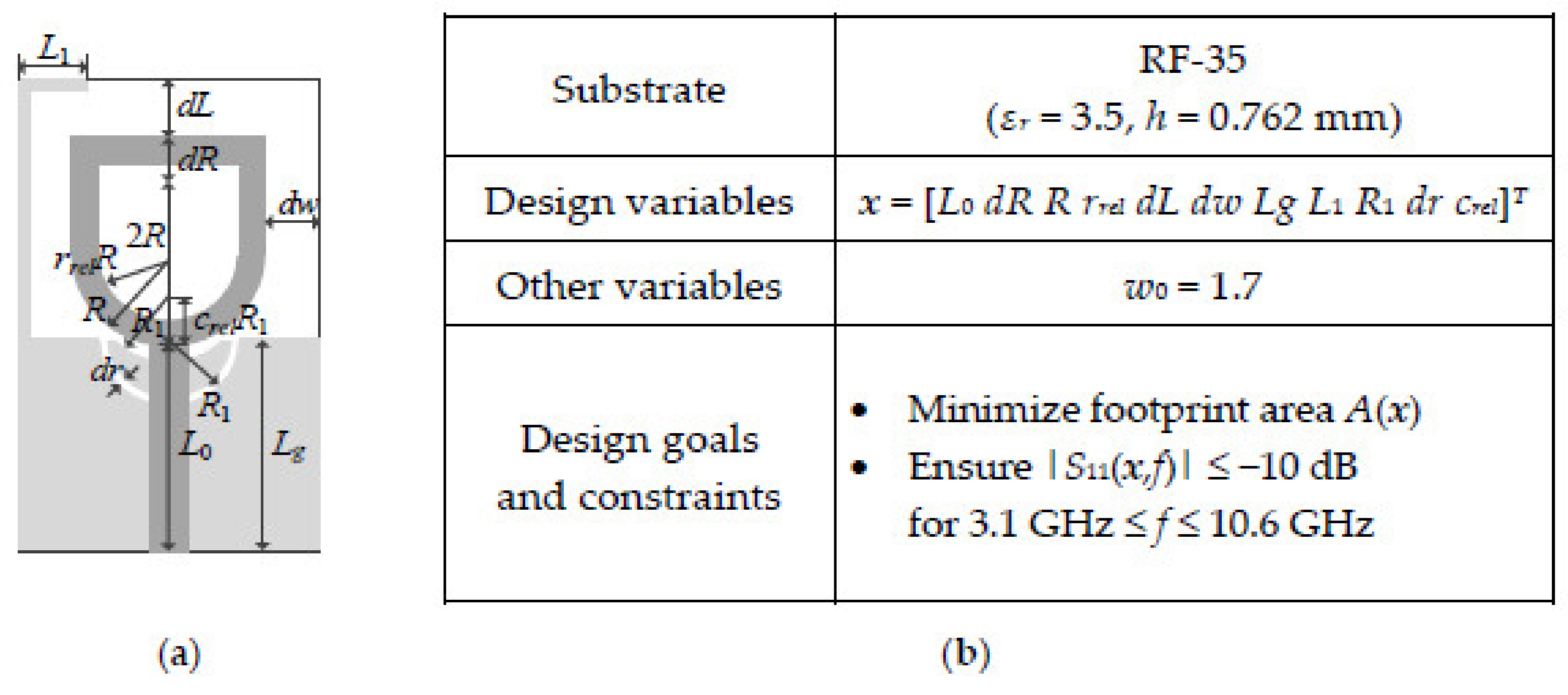
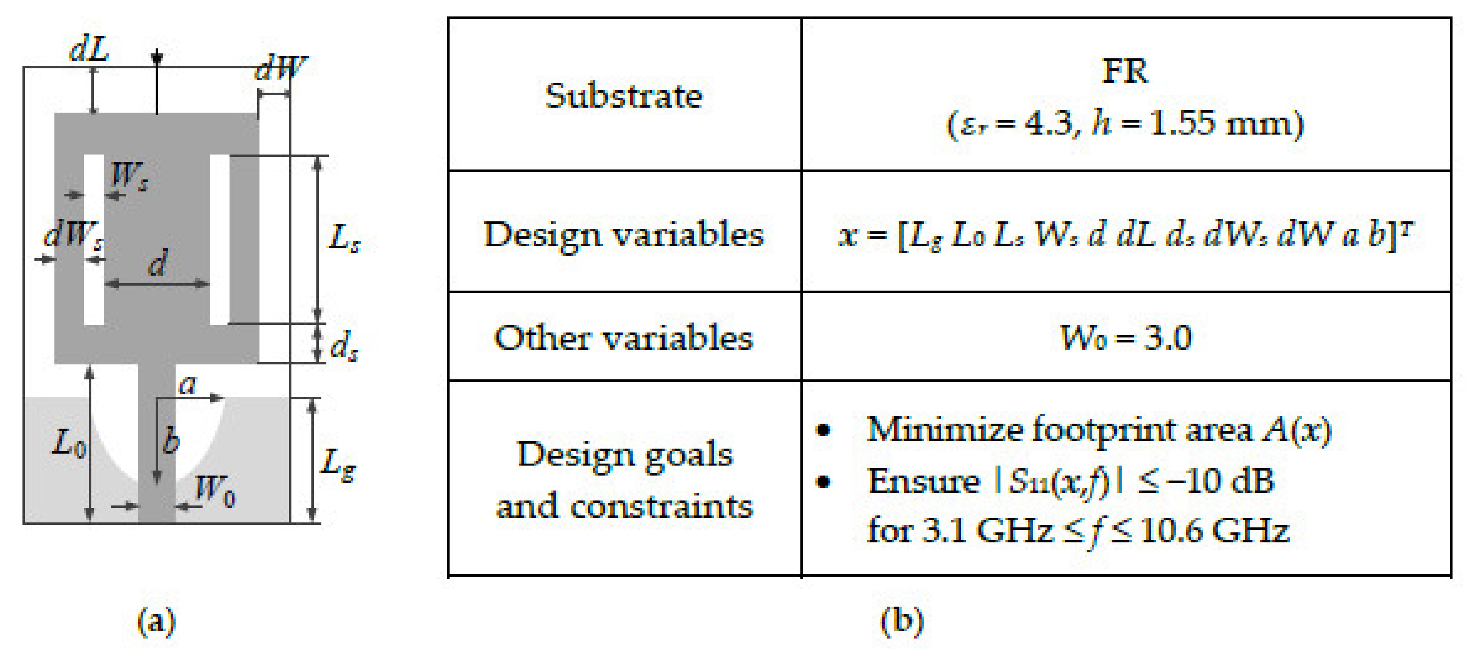
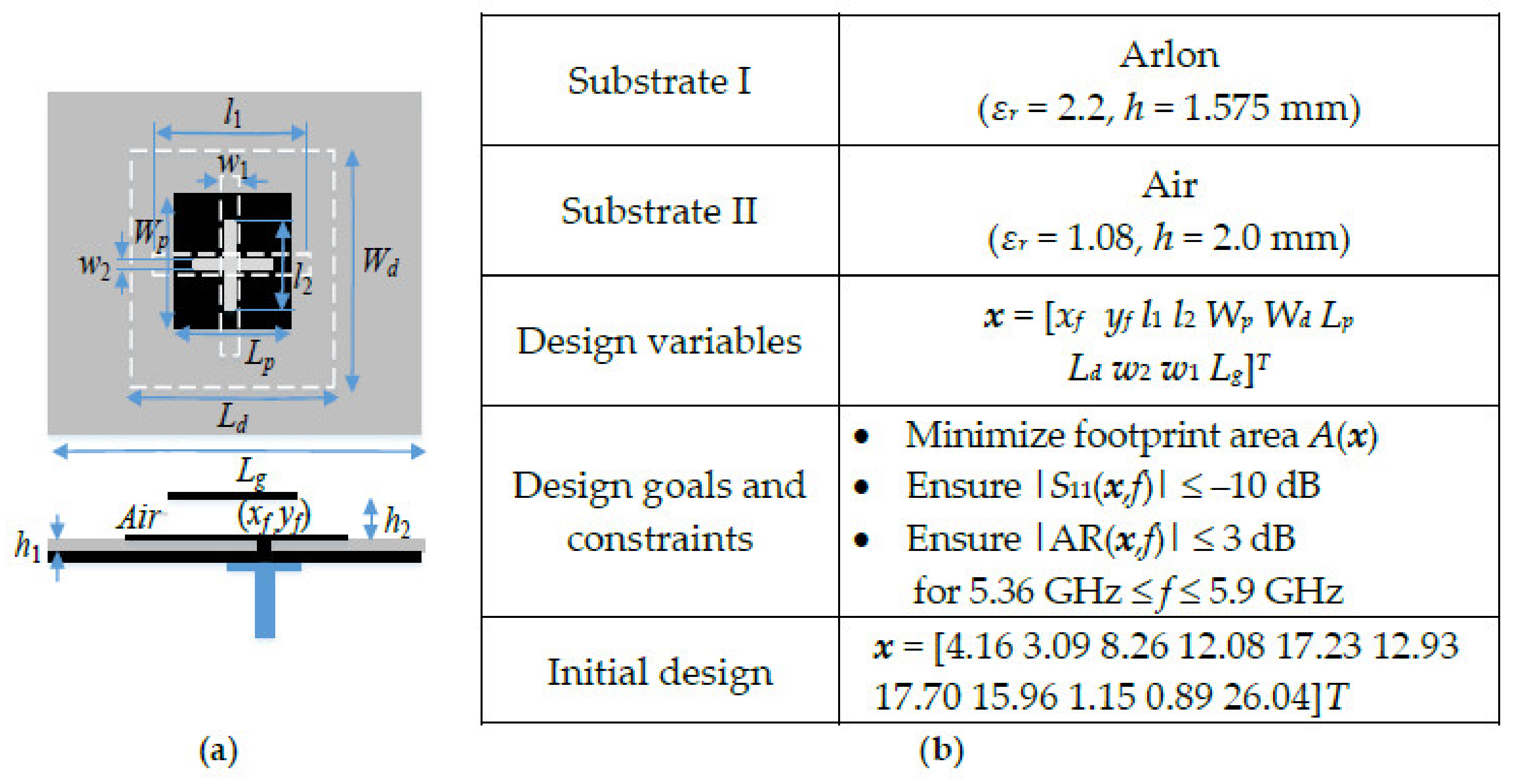
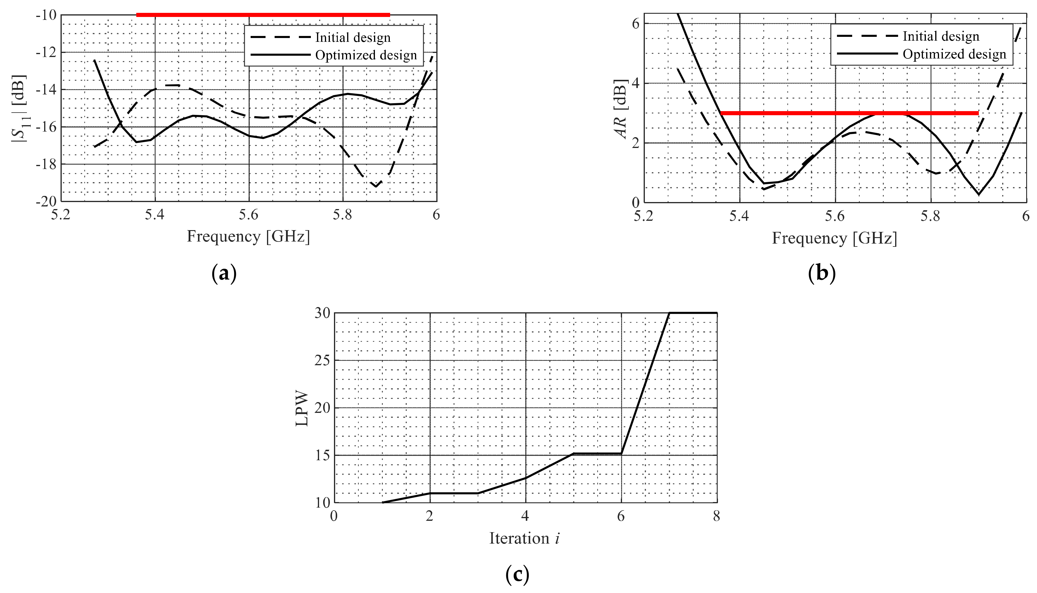
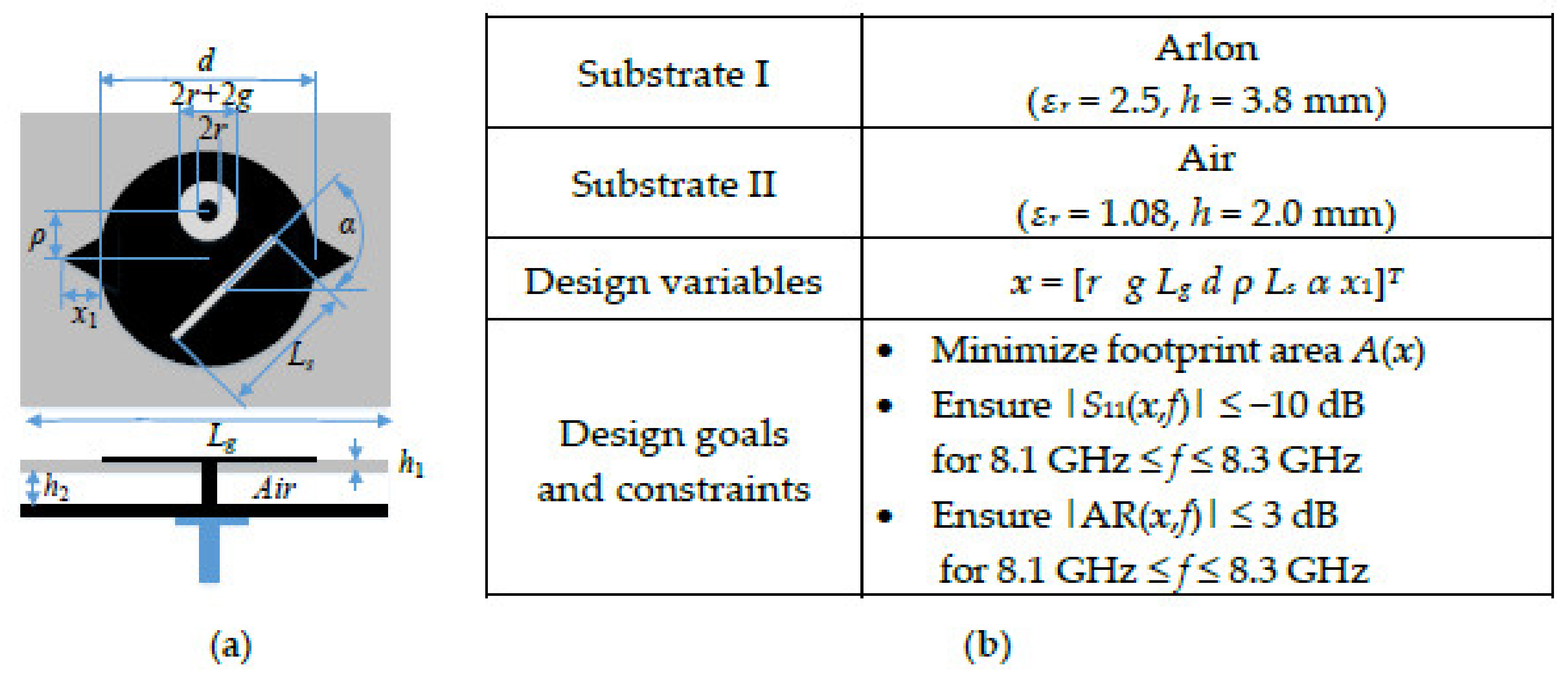
  • The reflection coefficient of the antenna should not exceed −10 dB within the frequency range F, i.e., |S11(x, f)| ≤ −10 dB for fF (inequality constraint);
  • Axial ratio AR should not exceed 3 dB within the frequency range F, i.e., |AR(x, f)| ≤ 3 dB for fF (also an inequality constraint);
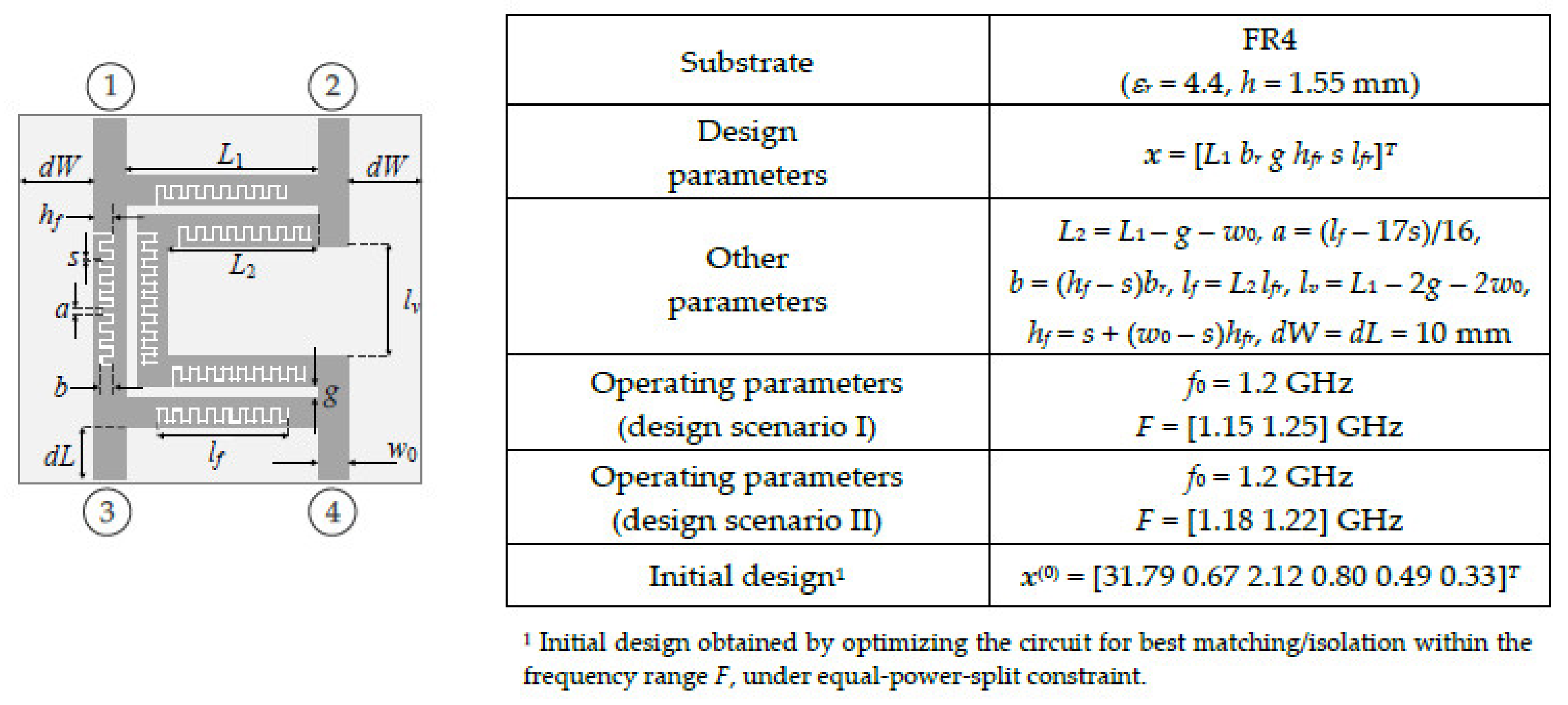
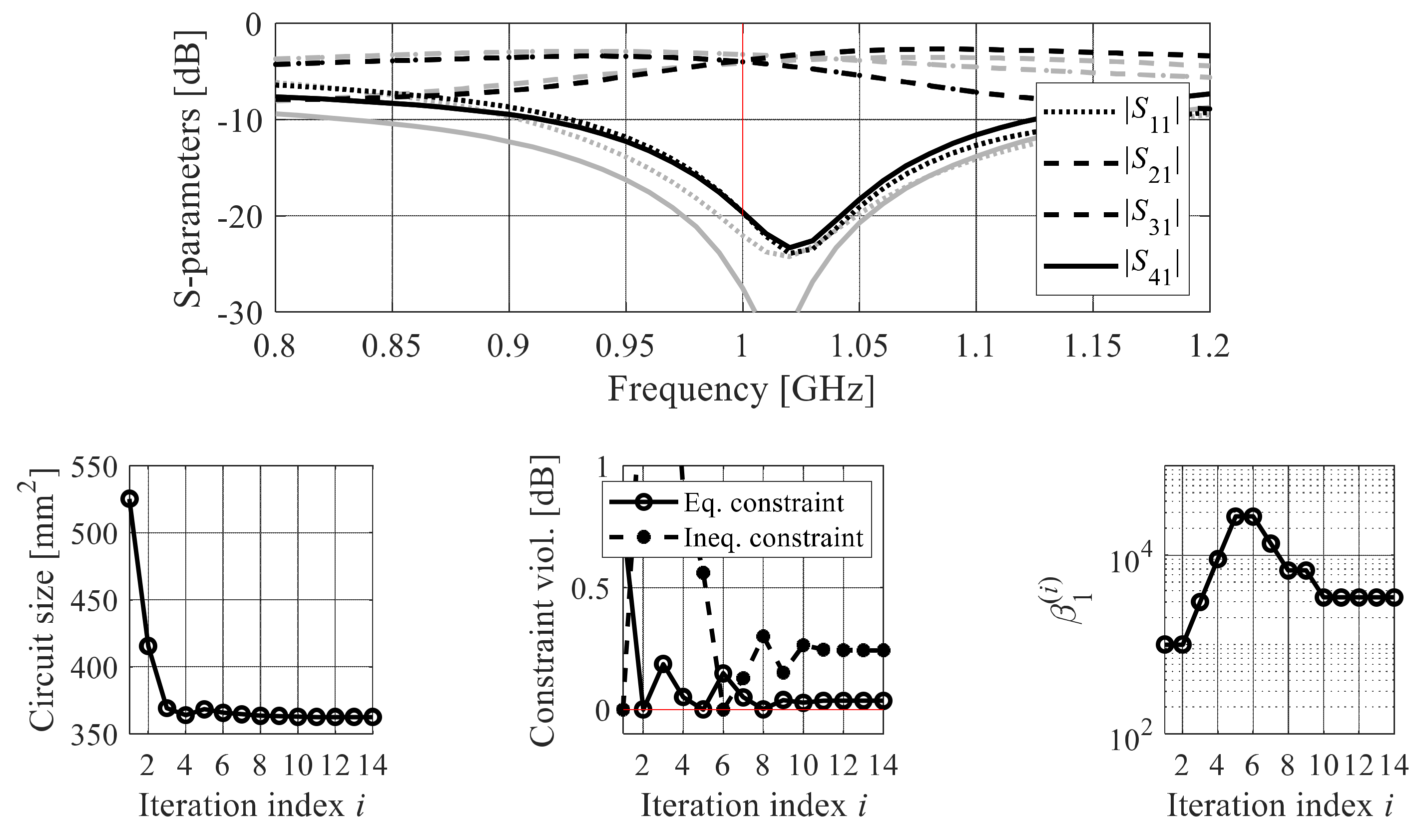
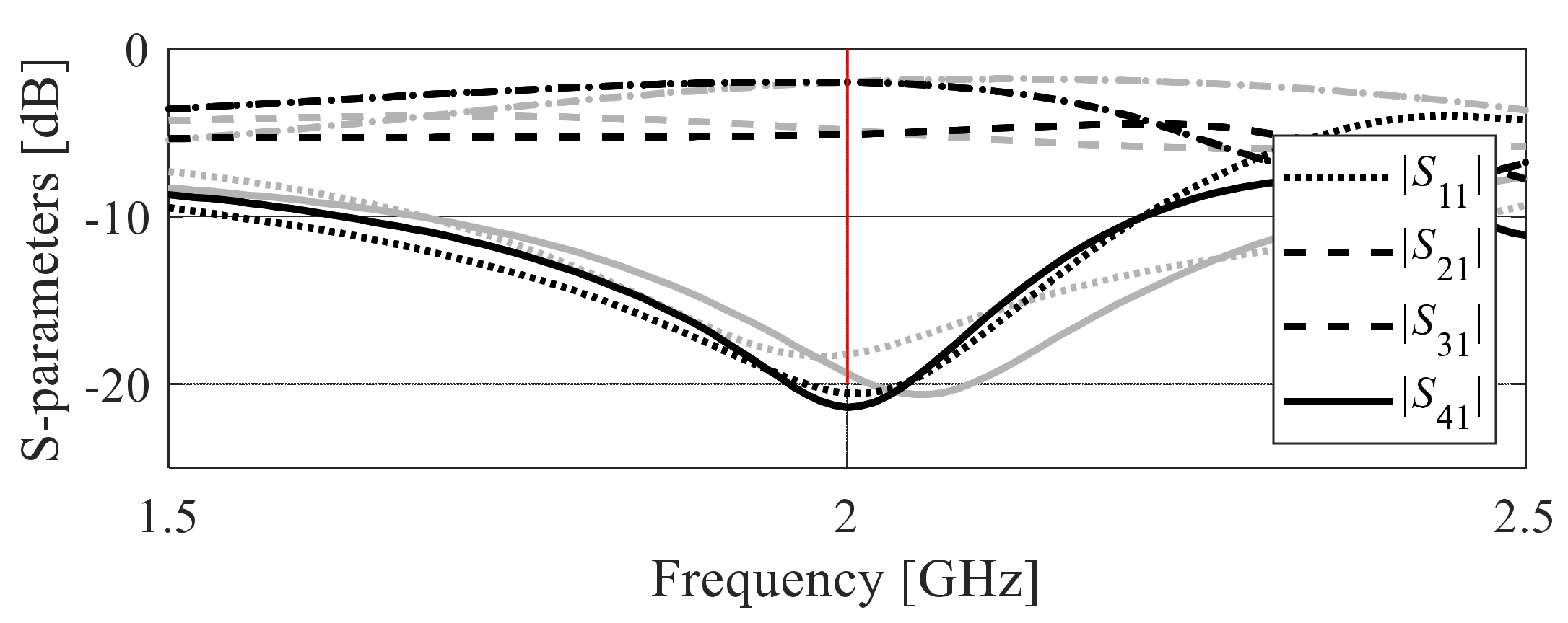
  • Power split ratio of a coupling structure KP should be equal to zero at the center frequency f0, i.e., KP = |S31(x, f0)| − |S21(x, f0)| = 0 dB (equality constraint)
Unfortunately, miniaturization is detrimental to the electrical and field performance of high-frequency structures [53]. Consequently, minimum-size designs are normally allocated at the feasible space boundary ∂Xf as at least one of the constraints is active at the optimum. Explicit treatment of design constraints (2) and (3) is often problematic, due to numerical issues related to the exploration of ∂Xf. An alternative is implicit handling using a penalty function approach [39]. The design task is then reformulated into
x * = arg min x   U p ( x )
where the objective function is defined as
U p ( x ) = A ( x ) + k = 1 n c β k c k ( x ) 2
In (5), minimization of A(x) is the primary objective, whereas the remaining terms are penalty factors that provide a non-zero contribution if the respective constraints are violated. The penalty function cj(x) is typically defined to quantify relative violations. For example, we may define cj(x) = max{0, [Sineq.j(x) – sj]/sj} for the jth inequality condition (3). Note that problem (4) is formally unconstrained, which facilitates handling of the size reduction task. On the other hand, the choice of the penalty coefficients βj is instrumental in the success and reliability of solving (4) and (5). As mentioned in Section 1, using too low or too high values leads to either the lack of constraint violation control or to numerical issues due to the steepness of the objective function Up in the vicinity of the feasible region boundary. The algorithms outlined in the remaining part of this paper attempt to address this and other difficulties of EM-driven miniaturization, both in the explicit and implicit constraint handling regimes.

3. Adaptive Penalty Function Methods

In a conventional penalty function approach, appropriate values of the penalty coefficients are adjusted on a trial-and-error basis and kept fixed throughout the entire optimization run. As mentioned on several occasions, such a setup is far from optimal, as it leads to obtaining inferior solutions, either in terms of an insufficient constraint control, or degraded values of the primary objective. In contrast, the adaptive penalty function methods monitor the levels of current constraint violations during the optimization run and adjust the values of the penalty coefficients accordingly. This allows for improving the reliability of the optimization process, as well as the precise control of constraints violation. This section outlines two versions of the algorithms exploiting an adaptive adjustment of penalty factors. In the first one, the penalty factor values are adjusted based on an appropriately quantified combination of the algorithm convergence status and the constraint violation level [42]. Whereas the second technique takes into account the improvement of constraint violation between consecutive algorithm iterations as well as solution feasibility [41].

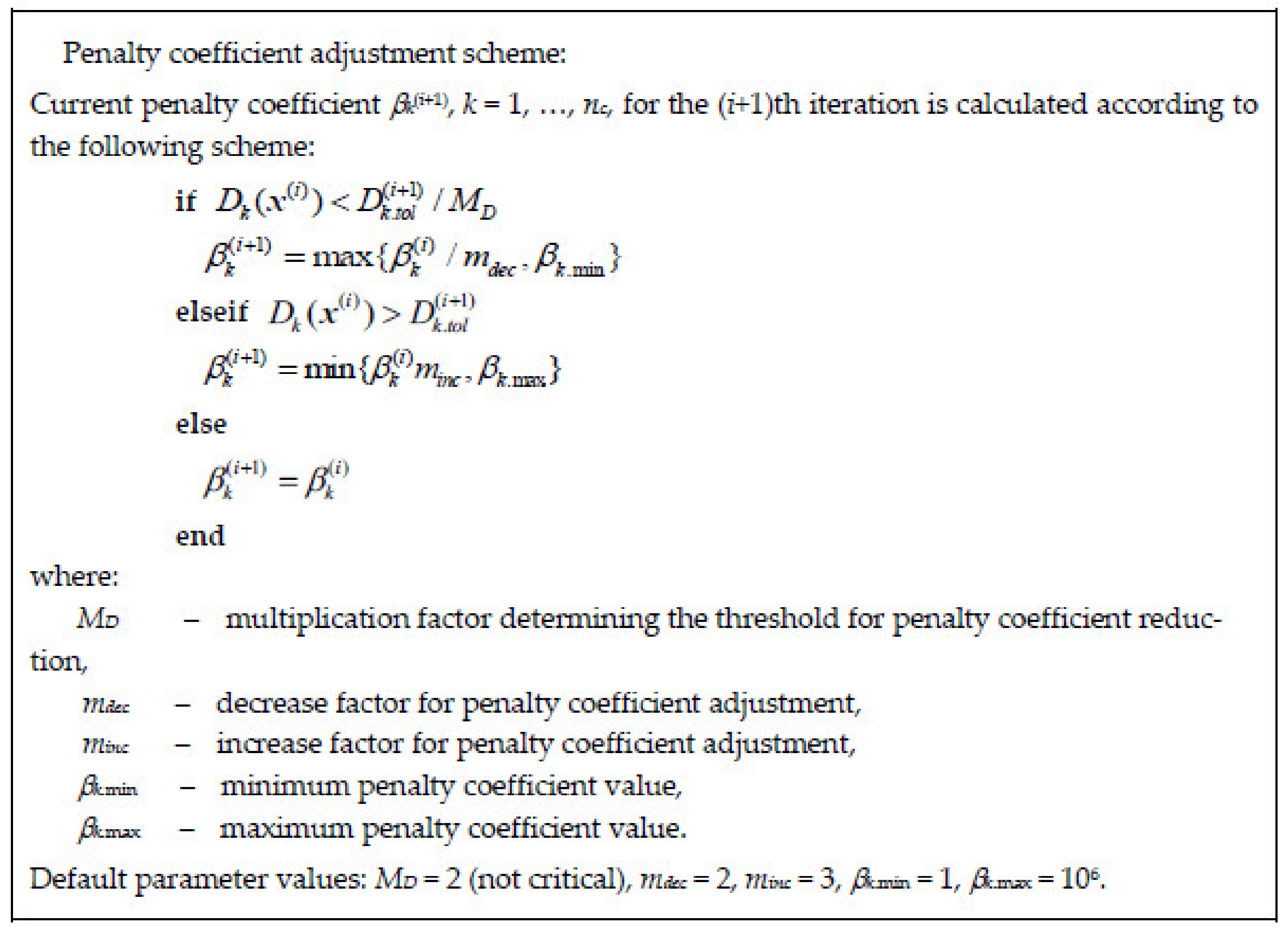
3.1. Adaptive Scheme I. Convergence Status and Constraint Violation Levels

The algorithm with automated adjustment of the penalty factors [42] adheres to the following assumptions: (i) the optimization process is initiated with low values of the penalty terms and increased tolerance thresholds for constraint violations to facilitate exploration of the design space, (ii) in the subsequent stages of the optimization run, the penalty coefficients are gradually increased, (iii) near convergence, the constraint violation tolerances are made more rigid to ensure the target levels of the constraint violations.
Overall, throughout the algorithm run, adaptive adjustment of both constraint violation tolerance thresholds and the penalty coefficient values is carried out, which are briefly explained in Figure 1 and Figure 2, respectively. A detailed exposition of the adaptive penalty factors adjustment, along with the discussion of the suggested setup of the algorithm control parameters can be found in [42].

3.1.1. Trust-Region Gradient-Based Algorithm

The approach of [42], as well as all other optimization procedures outlined in this paper, are embedded in the trust-region (TR) framework [54], which, for the convenience of the reader, is briefly outlined in this section. Let us recall that the TR algorithm yields a series of approximations x(i), i = 0, 1, …, to the optimum design x* of (1), where x(i) is found as
x ( i + 1 ) = arg min x ; | | x x ( i ) | | d ( i ) U L ( i ) ( x )
Here, UL(i) is the local (usually linear) model of the objective function Up at x(i). The problem is subject to constraints (2) and (3), although for notational simplicity we only assume inequality constraints here. The adjustment of the trust-region size d(i) is addressed below.
Denoting by r(x) the aggregated vector of EM-simulated system responses, consider a local expansion model L(i)(x) of r(x) set up at x(i)
L ( i ) ( x ) = r ( x ( i ) ) + J ( x ( i ) ) ( x x ( i ) )  
The Jacobian matrix J(x(i)) of r is estimated using finite differentiation. When considering individual components, the merit function can be expressed as
U L ( i ) ( x ) = A ( x ) + k = 1 n c β k ( i ) c L . k ( x )
where cL.k refers to constraint functions of the same form as ck of (4); yet, they are evaluated using the linear model L(i) of the component responses instead of directly from r.
The interval [x(i)d(i), x(i) + d(i)] of (6) is referred to as the trust region. Typically, its size is made proportional to the design space size, and its value in each algorithm iteration is decided upon using the standard TR rules [54] based on the gain ratio defined as
ρ = U P x i + 1 U P x i U L x i + 1 U L x i
The following rules for updating the TR region size apply: (i) if ρ > 0.75 (i.e., the gain ratio is large enough), d(i+1) is increased, (ii) if ρ < 0.25 (i.e., the gain ratio is small), d(i+1) is reduced, (iii) in other cases, it is remained intact. Furthermore, the next design is accepted only for ρ > 0, otherwise, the iteration is re-launched with a smaller d(i+1).

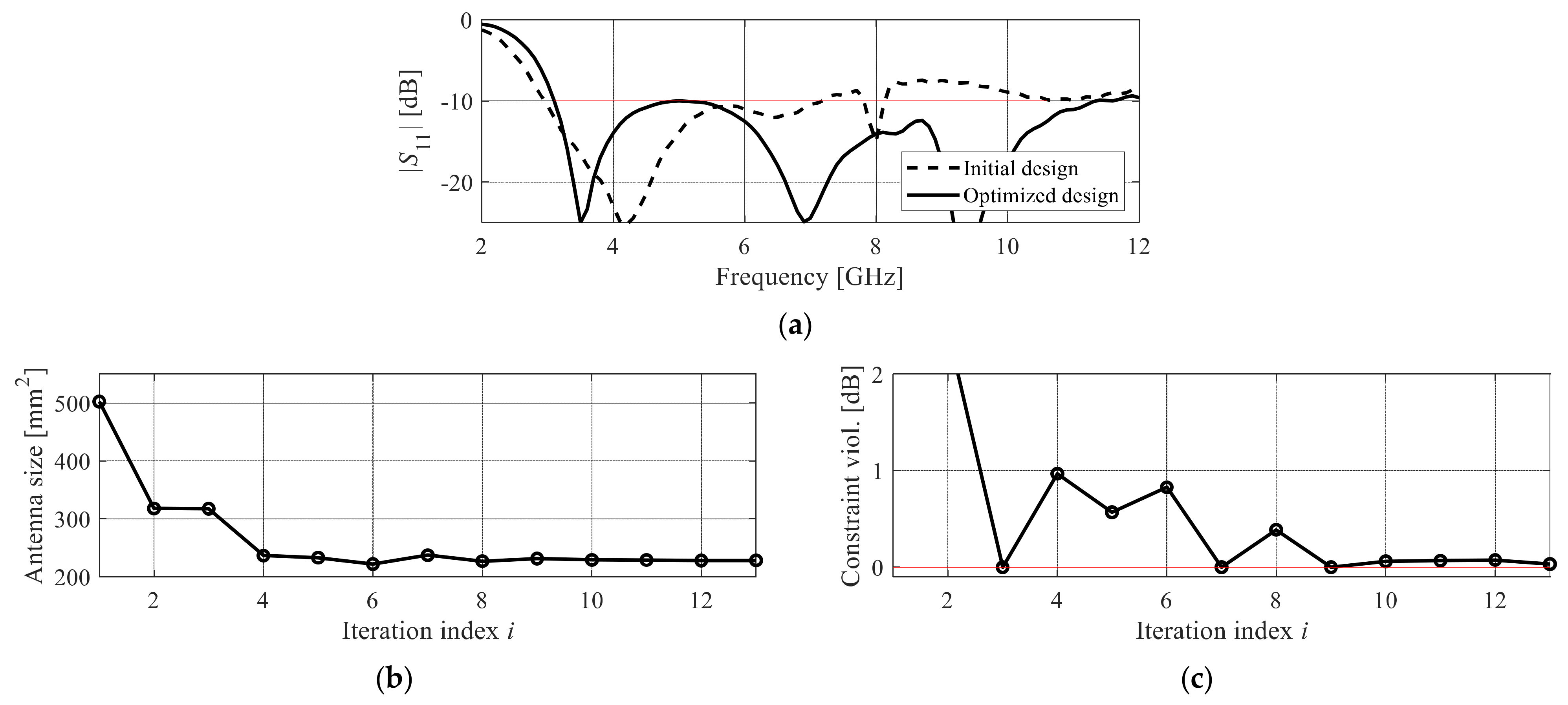
3.1.2. Example: Ultrawideband Antenna

Consider an ultrawideband antenna shown in Figure 3a. The structure parameters and design goals along with constraints are provided in Figure 3b. The antenna EM model is evaluated using CST Microwave Studio and incorporates the SMA connector (~1,200,000 mesh cells, simulation time 240 s). All the simulations were performed on Intel Xeon 2.1 GHz dual-core CPU with 128 GB RAM. The results obtained with the use of the algorithm [28] are compared to the fixed setup with different values of penalty factors. The procedure [42] has been executed with the default values of the control parameters given in Figure 2.
The discussed optimization task is a multimodal one; thus, a statistical assessment of the algorithm [42] is carried out based on ten independent runs, executed using random initial designs. Table 1 provides the optimization results in the form of the average values of antenna size and constraint violations, along with standard variation thereof. Antenna reflection characteristics and the evolution of penalty coefficient values for a representative algorithm run are shown in Figure 4. The results of Table 1 indicate that the miniaturization framework of [42] allows for precise constraint control. In addition, for similar average constraint violation levels, the adaptive penalty factors approach renders antenna designs with improved miniaturization rates.

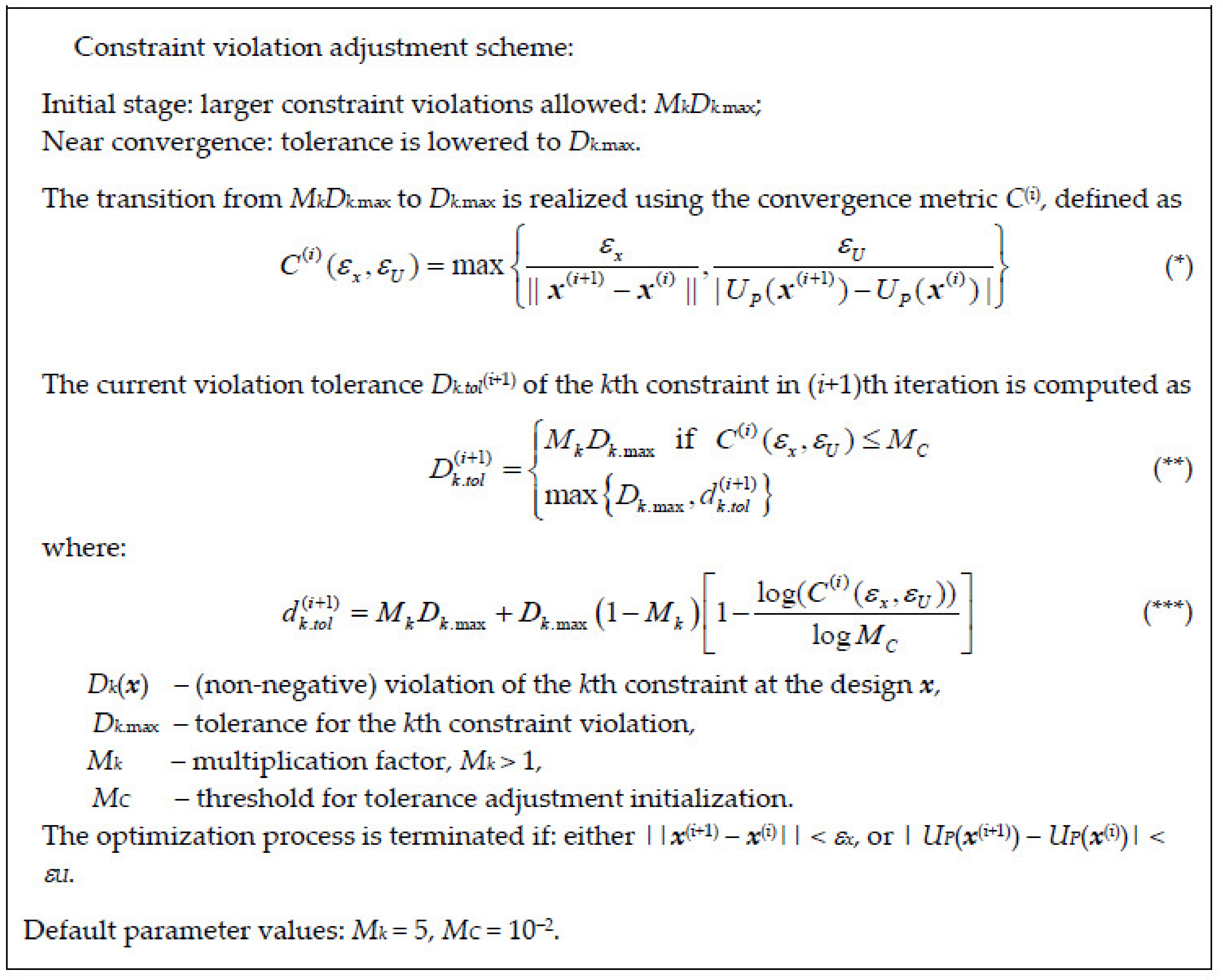
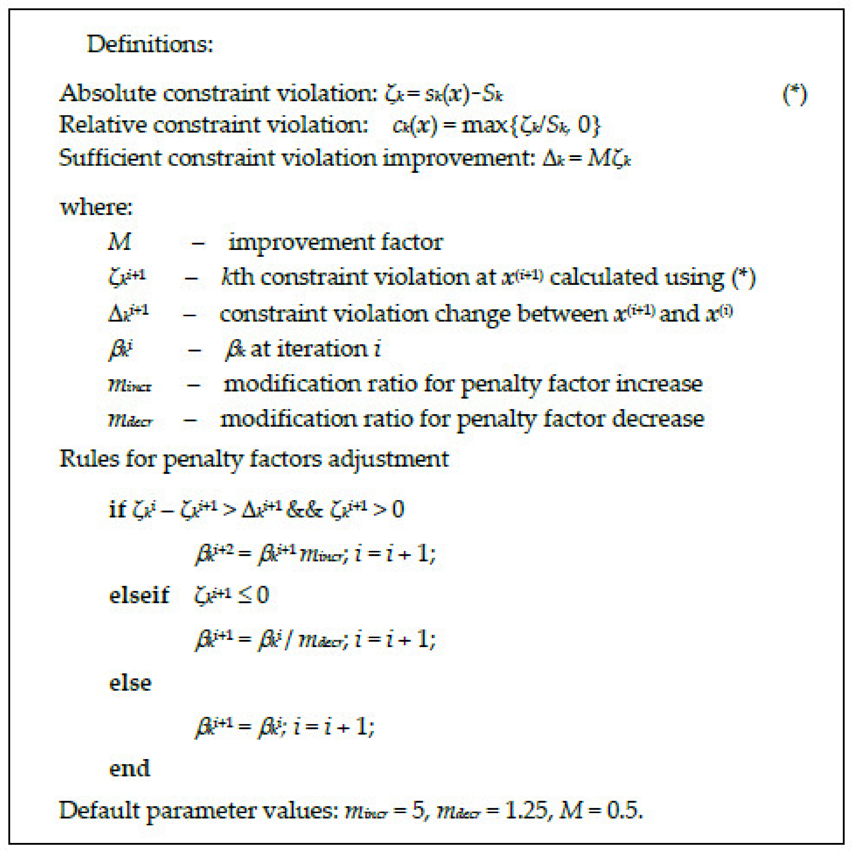
3.2. Adaptive Scheme II. Sufficient Constraint Violation Improvement

An alternative adaptive penalty coefficient methodology has been proposed in [41]. It exploits a somewhat different approach than the technique delineated in Section 3.1. In [41], the adjustment of the penalty factors is based on monitoring both the feasibility status of the current design and the improvement of the constraint violation between algorithm iterations. The rules for governing the current values of the penalty coefficients, along with basic definitions of the technique [41], are shown in Figure 5.
In [41], the penalty functions of (5) quantify relative violations of the constraints, whereas the penalty coefficients serve to commensurate the contribution of the said relative constraints to the primary objective (i.e., footprint area of the component under design). In [41], the inequality constraints take the form
sk(x) ≤ Sk, j = 1, …, nineq
In short, the operation of the algorithm [41] may be described as follows. If the current design is feasible with respect to the kth constraint, the corresponding penalty factor is reduced. If, however, the actual design is infeasible but, at the same time, the constraint violation has been sufficiently improved, the previous value of the penalty coefficient is retained to maintain the optimization process stable. In the case of infeasible current design accompanied by insufficient constraint improvement, the respective penalty factor is increased.

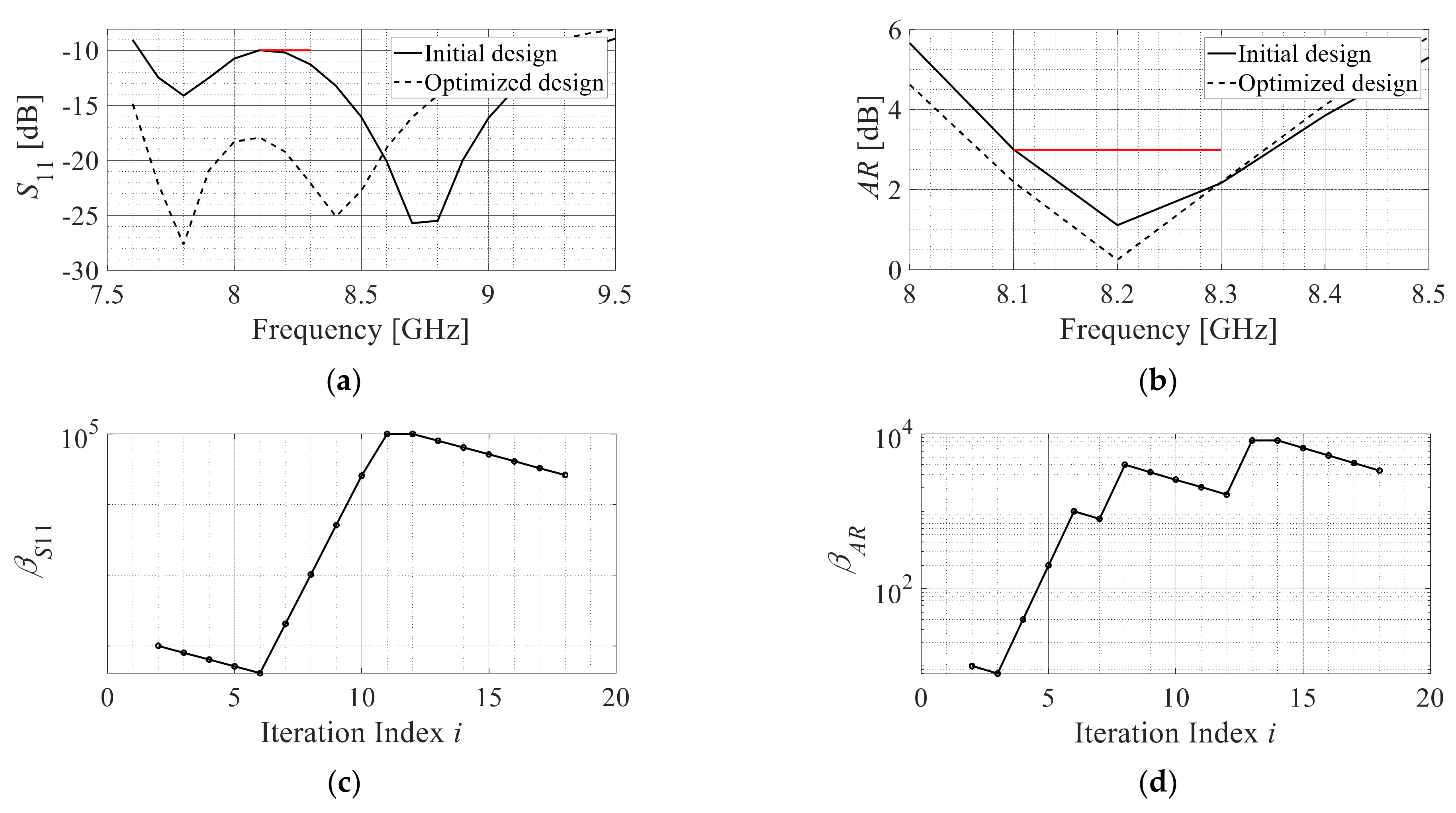
Example: Circular Patch Antenna

Figure 6a shows a circularly polarized antenna used as a verification case in [41]. The antenna parameters, substrates and design goals/constraints are given in Figure 6b. The antenna EM model is evaluated using a time-domain solver of CST Microwave Studio (~400,000 mesh cells, simulation time 150 s). The results obtained with the approach of [41] are benchmarked against the fixed setup with different values of penalty factors.
Table 2 shows the optimization results: the antenna footprint, as well as violations of both constraints ζAR and ζS11, imposed on axial ratio and reflection, respectively. Figure 7 shows the antenna outputs, along with the evolution of penalty factors throughout the optimization run. Similarly, as for the algorithm described in Section 3.1, the considered procedure allows for obtaining enhanced miniaturization rates, and, at the same time, a better level of control over constraint violations has been achieved.

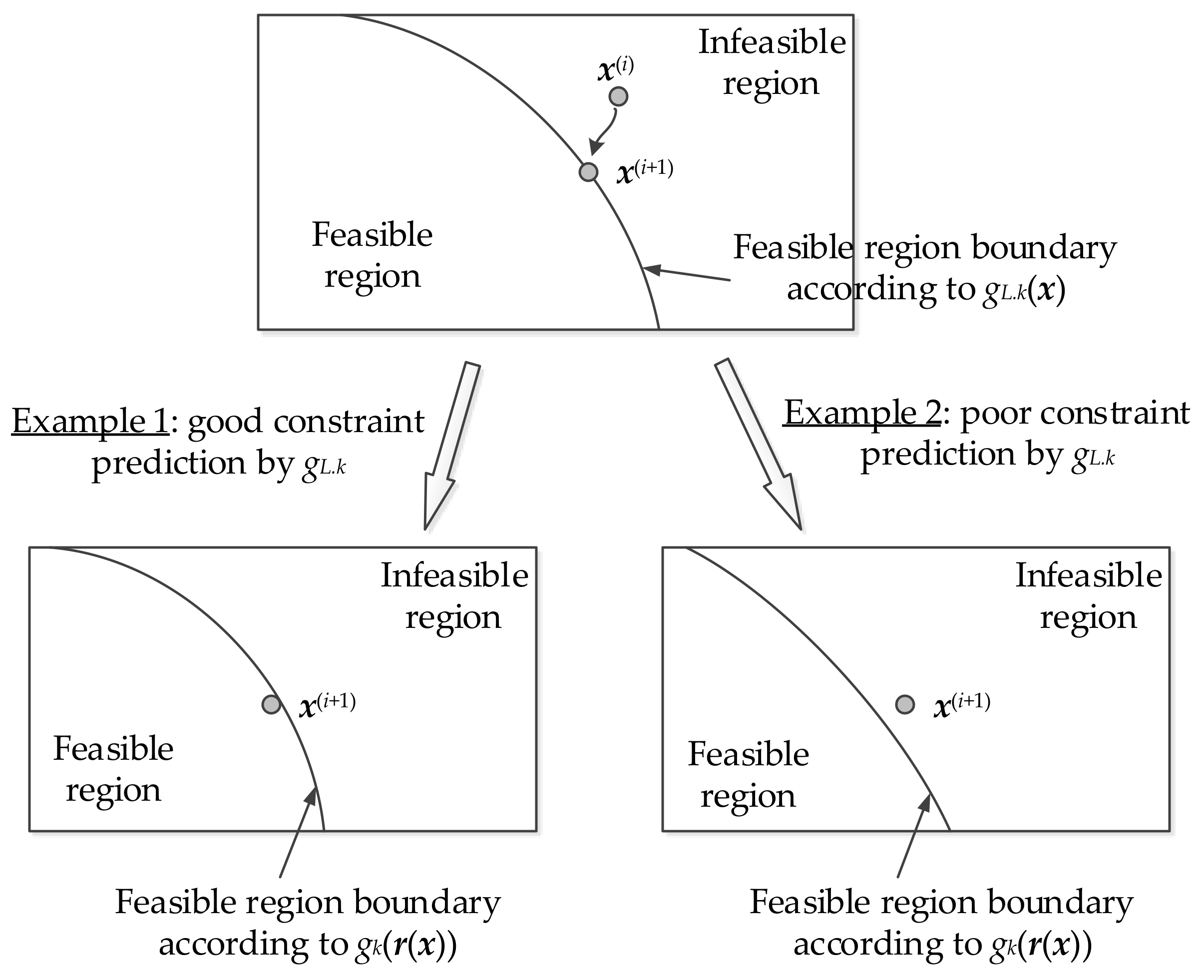
4. Explicit Constraint Handling Approach

The implicit approach can alleviate some of the difficulties pertinent to the handling of computationally expensive design constraints while creating problems of its own. As elaborated in Section 2, the appropriate choice of the penalty coefficients is critical for the performance of the optimization process. Section 3 outlined two strategies for adaptive adjustment of those coefficients, which enable relatively precise control of the constraints while ensuring competitive miniaturization rates. It should be noted, however, that implementation of these strategies is rather complex. Recently, a technique for explicit constraint control in high-frequency design has been presented [44], which operates on entirely different principles while enabling similar benefits as the procedures of [41,42]. This section outlines this approach and illustrates it using two examples.

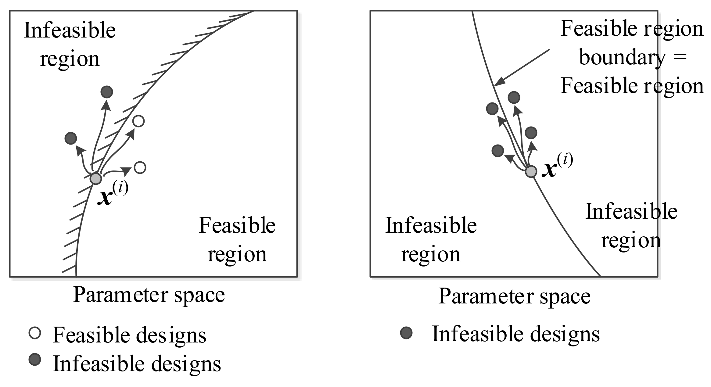
4.1. Explicit Constraint Handling

The approach of [44] is embedded in the trust-region (TR) framework [54] briefly outlined in Section 3.1. In [44], the following model of the kth constraint Sineq.k(r(x)) is used:
S L . i n e q . k ( x ) = S i n e q . k ( L ( i ) ( x ) )
The new point x(i) is found using (2) subject to SL.ineq.k(x) ≤ 0, k = 1, …, nineq.
The keystone of the procedure [44] is the updating scheme for the trust-region size d(i). It has been explained in Figure 8. Good alignment between the linear-model-predicted constraint value SL.ineq.k(x) and the actual value Sineq.k(r(x)) promotes the increase in d(i), whereas poor agreement results in decreasing it.

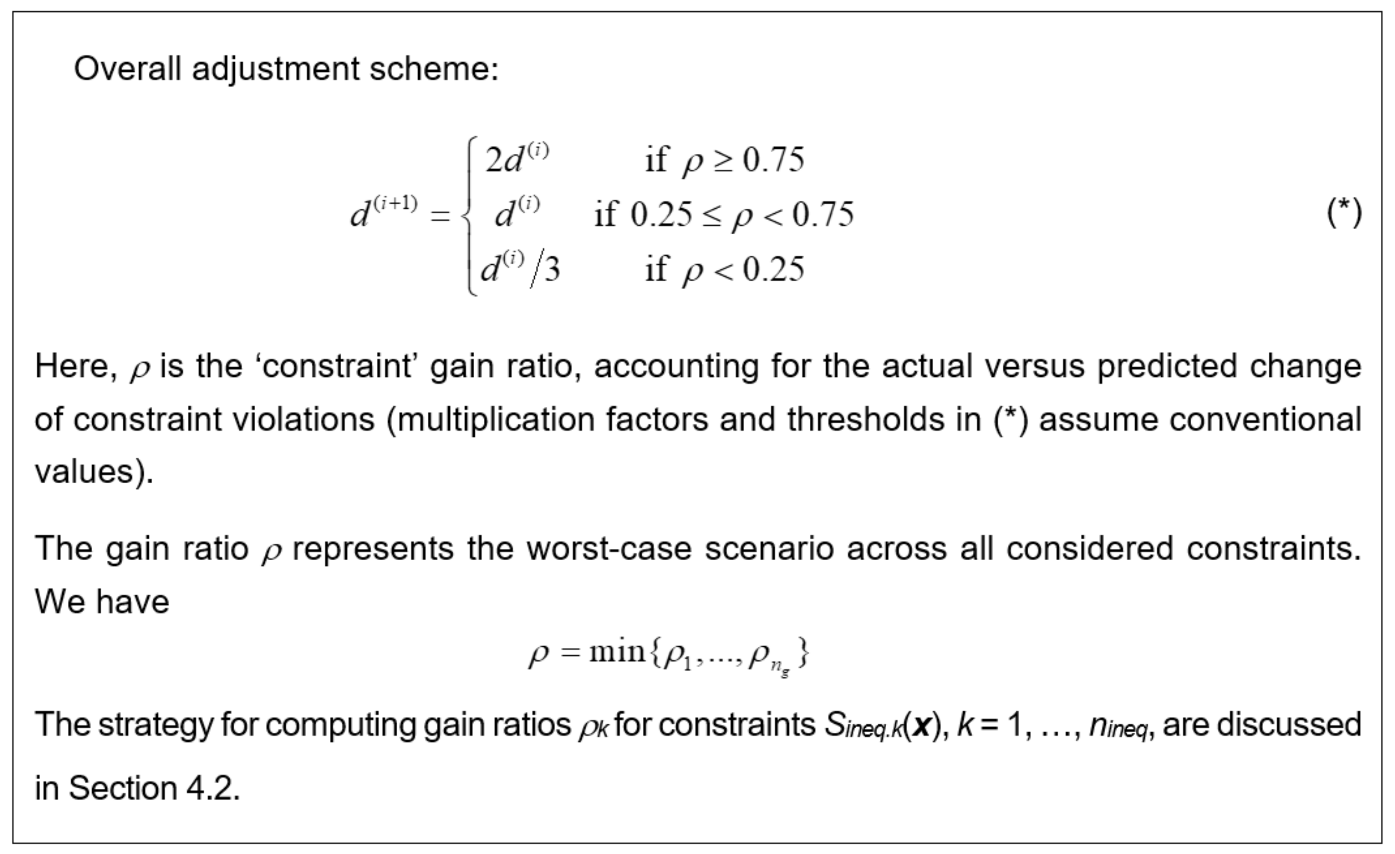
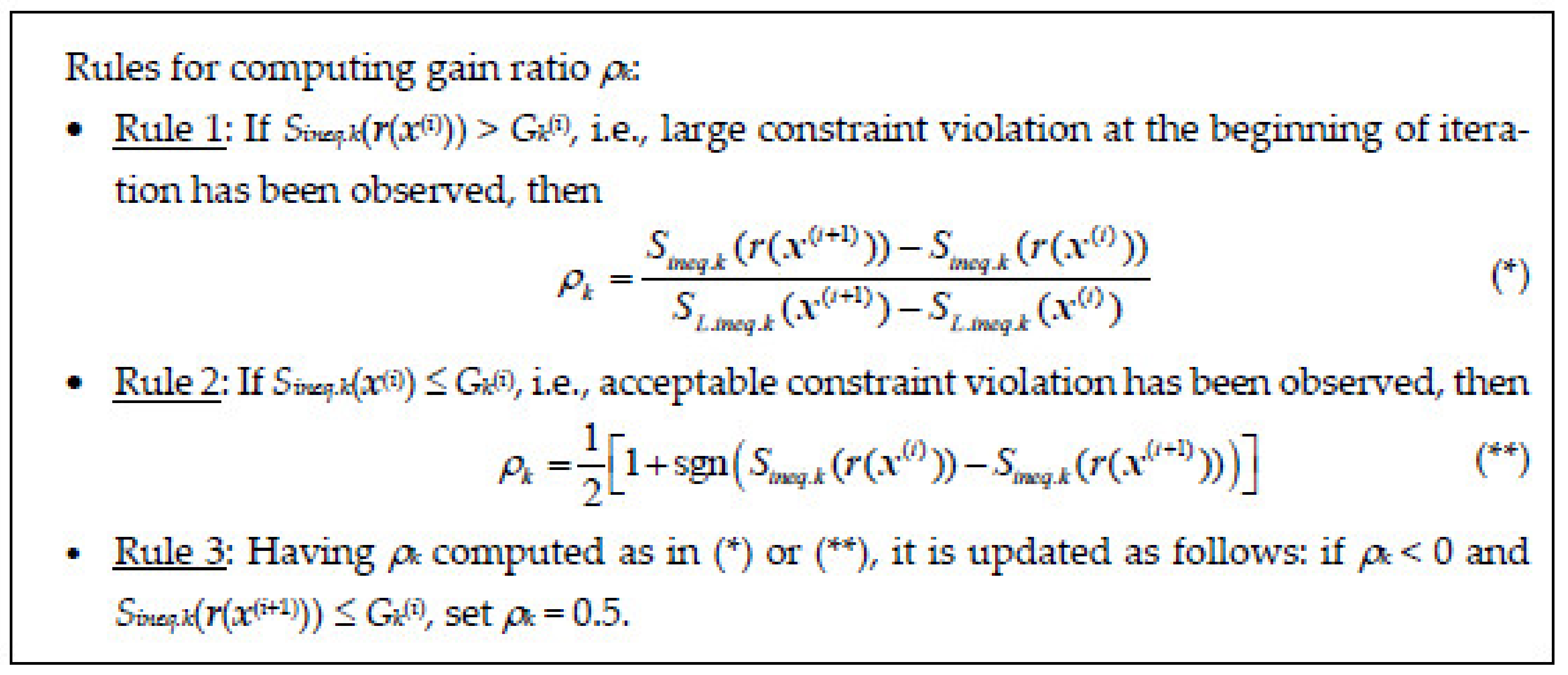
4.2. Calculating Gain Ratio

Figure 9 shows the rules for computing the gain ratio considered in Figure 8. Their evaluation is contingent upon the acceptance threshold Gk(i) set up for the constraint k at iteration i. Rules 1 and 2 penalize insufficient prediction of constraints of the linear model GL.ineq.k for sizeable constraint violations, and no improvement of feasibility status for minor violations, respectively. The same rules promote satisfactory prediction capability, and design shifts towards feasible regions. Rule 3 overrides both Rules 1 and 2 if the actual violation at x(i+1) is lower than Gk(i). This allows for avoiding erratic behavior in the vicinity of the feasible region boundary [44].
Some examples of poor and good constraint prediction can be found in Figure 10. Regarding the thresholds Gk(i), to allow more space for infeasible solutions early in the optimization process, the thresholds are associated with the algorithm convergence status, and the maximum acceptable constraint violation Gk.max (user-defined). Given the termination condition ||x(i+1)x(i)|| < ε or d(i) < ε (ε being the user-defined threshold) the convergence status at iteration i is defined as [44]
C ( i ) = max 1 , min | | x ( i + 1 ) x ( i ) | | , d ( i ) ε
The acceptance threshold for iteration i + 1 is set as
G k ( i + 1 ) = G k . max min 1 , α C ( i )
As C(i) is initially large, so is Gk(i+1). Near convergence, it is reduced to αGk.max, where α > 0 is a small number [44].

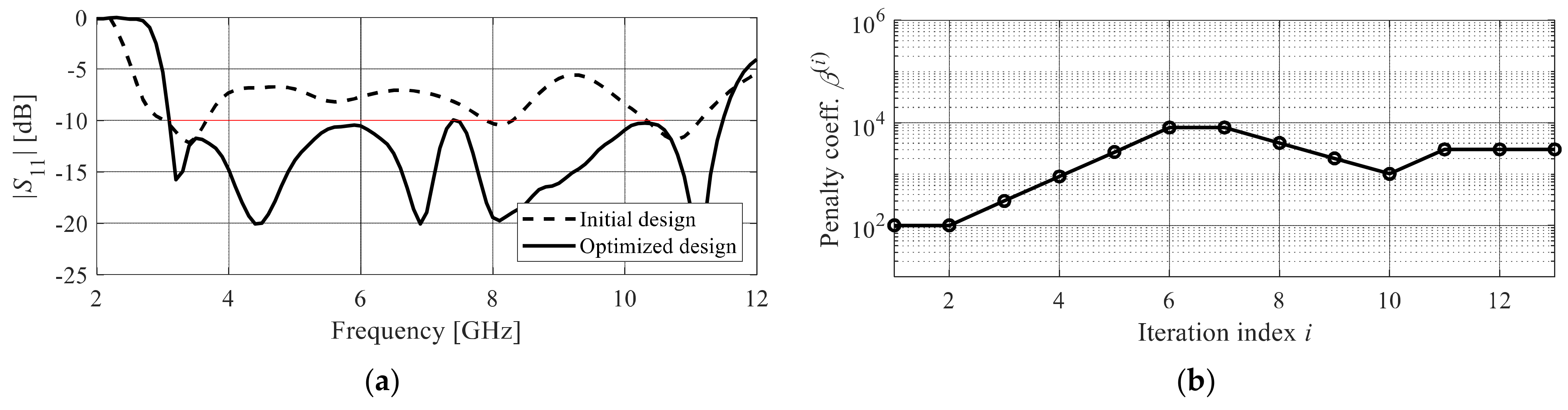
4.3. Example I: Broadband Antenna

Consider the broadband antenna shown in Figure 11a. The relevant parameters and design goals/constraints are specified in Figure 11b. The EM model is simulated in CST Microwave Studio and incorporates the SMA connector (~380,000 mesh cells, simulation time 100 s).
The algorithm of [44] is compared to several benchmark methods including the penalty function approach with fixed penalty coefficients and the adaptive scheme of [42]. The acceptance threshold is set so Gk.max = 1 dB with α = 0.1. The results are shown in Table 3 in the form of the average values of performance indicators and their standard deviations. Figure 12 shows the antenna reflection response, the size and constraint violation evolutions for a representative run of the algorithm. As it can be observed, the method of [44] enables the precise control of the design constraint and slightly improves the miniaturization rate in comparison to the penalty function approach (for commensurate average constraint violation levels). Explicit constraint handling is competitive to the adaptive approach of [42] with regard to tackling constraint violations, which leads to slightly increased average antenna sizes.

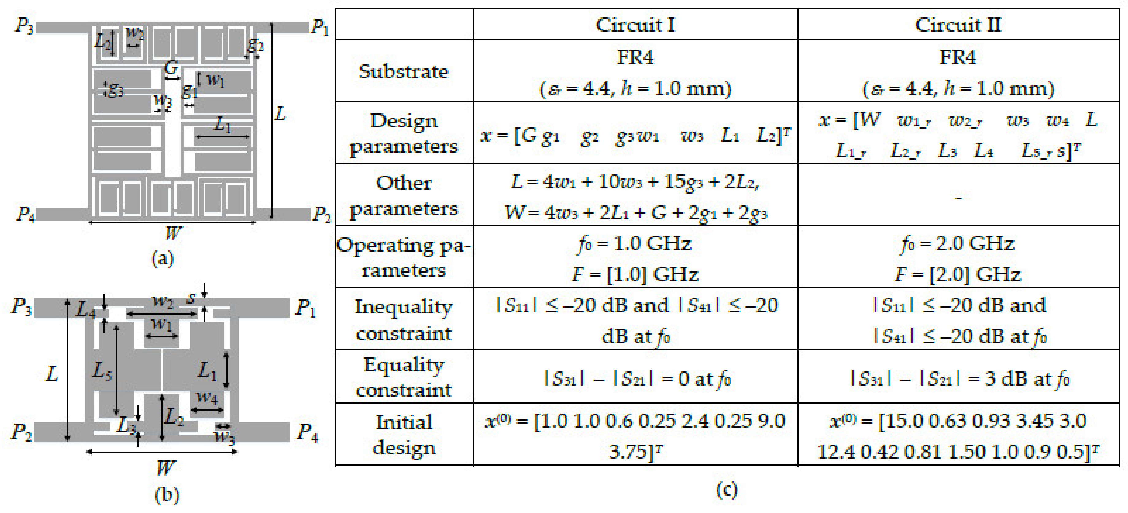
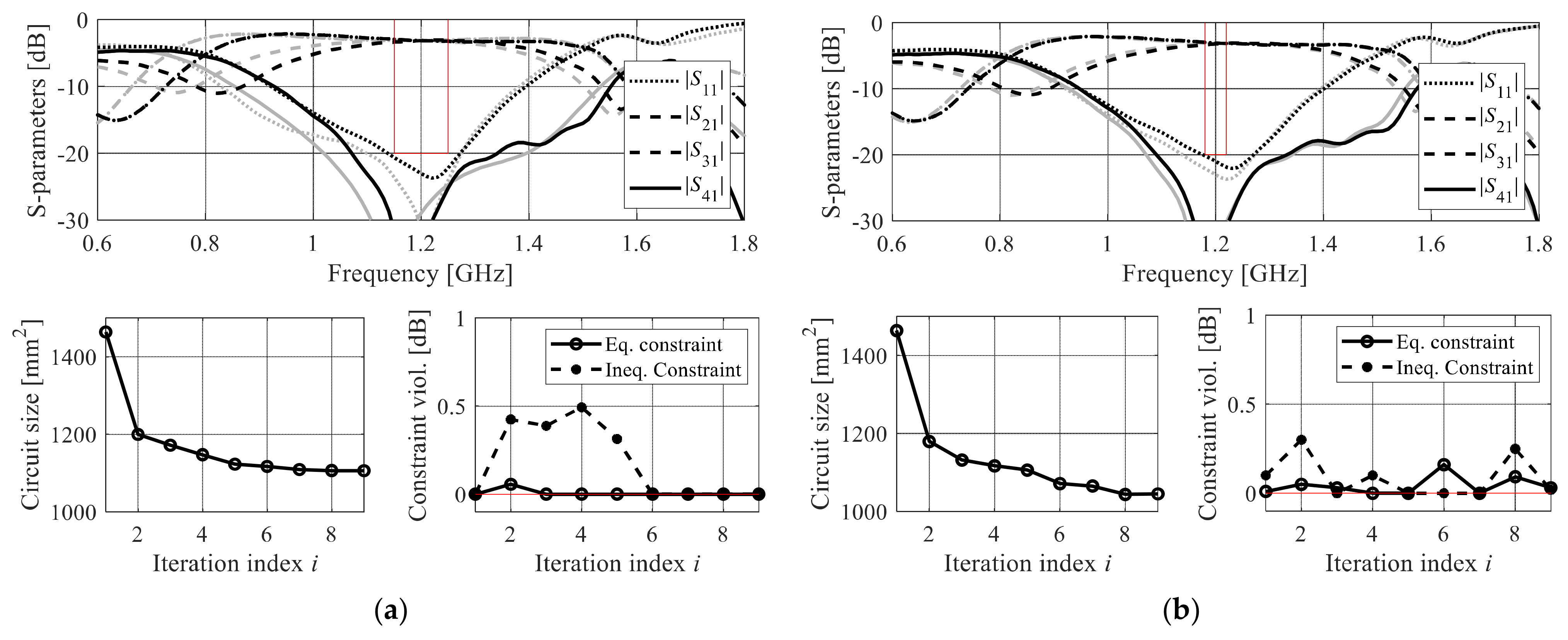
4.4. Example II: Rat-Race Coupler

Consider a rat-race coupler shown in Figure 13. Its EM model is simulated in CST Microwave Studio (~40,000 mesh cells, simulation time 180 s). The main objective is a reduction in the circuit footprint area. There are two design constraints: Seq.1(x) = ||S31(x, f0) − S21(x,f0)|| dB, and Sineq.1(x) = max{fF: max{|S11(x, f)|, |S41(x, f)|}} + 20 dB, where f0 is the center frequency, and F is the intended circuit bandwidth, for which we set up two scenarios as shown in Figure 13b.
The circuit size was optimized using the procedure of [43], and the algorithm used the implicit approach with a number of combinations of the penalty coefficients. The termination threshold is set to ε = 10−3, the acceptance thresholds are chosen to be G1.max = 1 dB, G2.max = 0.3 dB, and α = 0.1.
Table 4 shows the numerical results, whereas Figure 14 illustrates the circuit responses and the evolution of the footprint area and constraint violations during the optimization run. The algorithm of [43] performs consistently for both design scenarios. It does not only ensure precise control of the constraints (at the level of small fractions of dB) but also yields a design featuring competitive size, which is unlike the implicit approach with the manual setup of penalty coefficients. Note that if the number of constraints increases, the number of combinations of penalty coefficients increases as well, which makes their proper selection significantly more difficult.

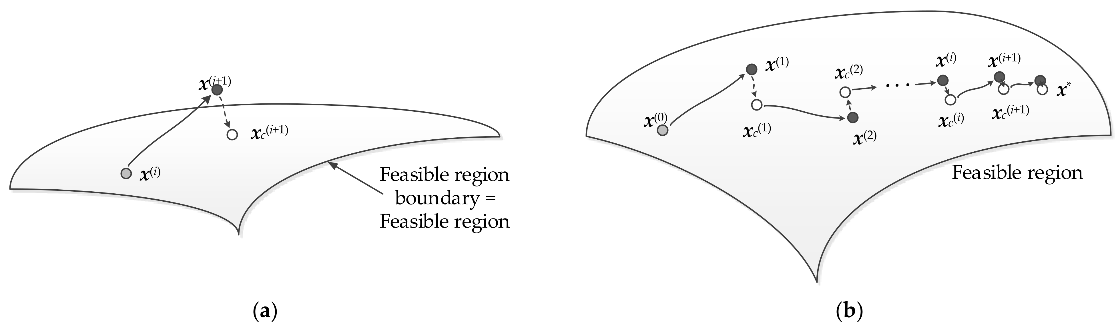
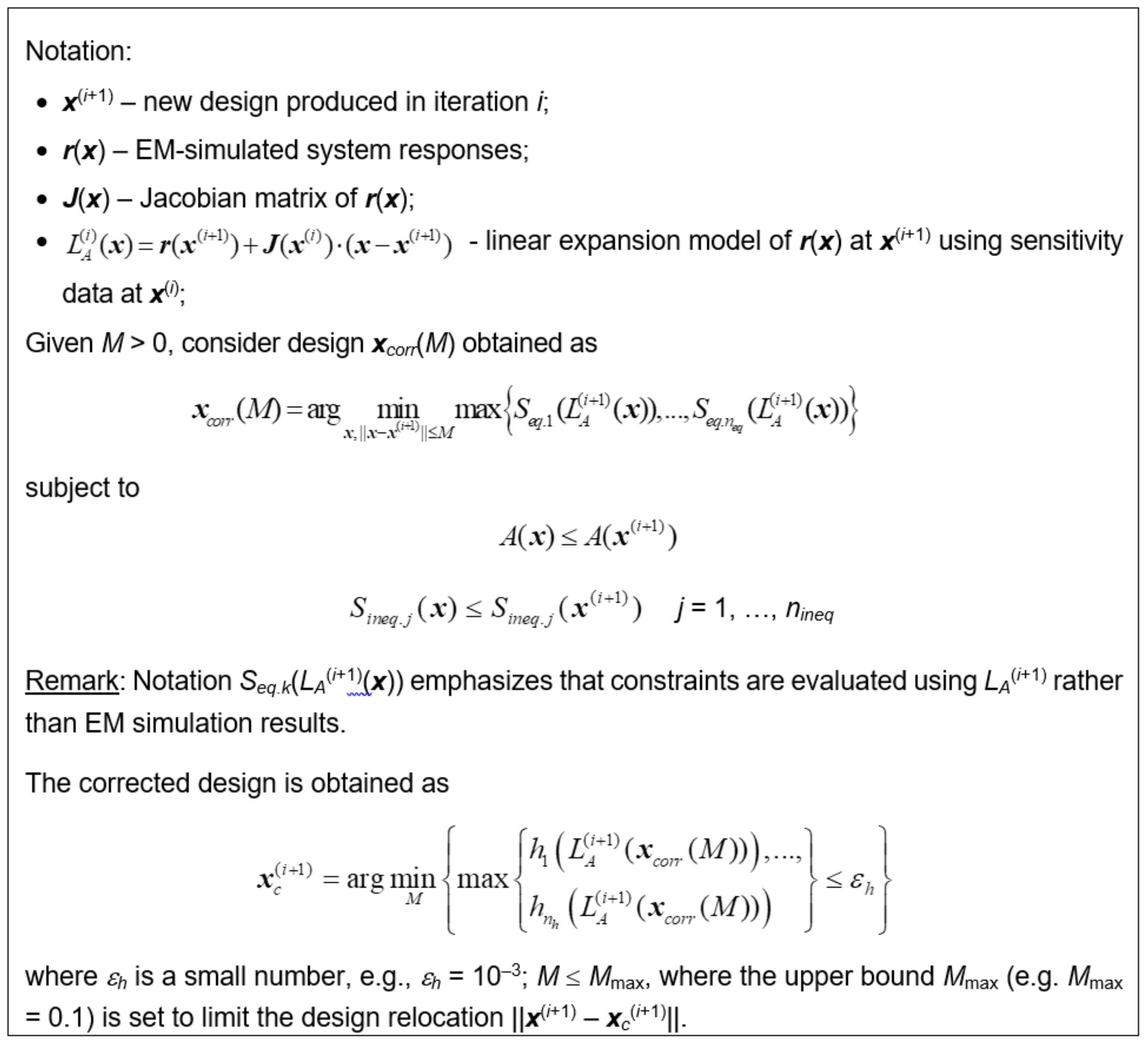
5. Equality Constraint Control through Optimization-Based Correction

The handling of equality constraints is more challenging than controlling inequality ones because the feasible region for the former is a thin set (i.e., it is identical to its boundary). Its exploration is difficult because any deviation from the boundary increases the (penalized) objective function, cf. Figure 15. Recently, a strategy for improved handling of equality constraints was proposed in [45], which is briefly outlined and illustrated in this section.

5.1. Correction Procedure

According to [45], the inequality constraints are handled by means of the adaptive scheme (e.g., [42]), whereas the equality constraints are corrected after each iteration of the optimization process. The correction process has been explained in Figure 16. It should be noted that the model LA(i) therein reuses the Jacobian J(x(i)) to reduce the cost of its establishment (upon convergence J(x(i)) → J(x(i+1)), so that LA(i) becomes closer to the true Taylor expansion at x(i+1)). As explained in Figure 17, the corrected design is obtained through possibly small relocation of x(i+1) to xc(i+1) aimed at reducing the equality constraint violation in the minimax sense without increasing A(x) and degrading inequality constraints.
The overall optimization procedure is embedded in the standard trust-region gradient-based framework with numerical derivatives [54]. For more details, see [45].

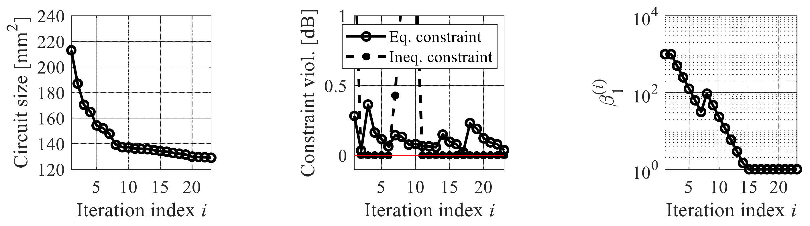
5.2. Illustration Examples

Consider two branch line couplers shown in Figure 18, where all the relevant data on both structures are provided. EM models are simulated in CST Microwave Studio (Circuit I: ~450,000 mesh cells, simulation time 300 s; Circuit II: ~112,000 mesh cells, simulation time 160 s). In both cases, the primary objective is a reduction in the circuit footprint A(x). Further, we have an inequality constraint for matching and port isolation, Sineq.1(x) = max{fF: max{|S11(x, f)|, |S41(x, f)|}} + 20 dB. This corresponds to a condition that both |S11(x, f)| and |S41(x, f)| should be not higher than −20 dB over the operating band F. We also have an equality constraint for the power split ratio: Seq.1(x) = ||S31(x, f0) − S21(x, f0)|| − KP, where KP is the required power split (in dB). Here, KP = 0 for Circuit I, and 3 dB for Circuit II.
The circuits’ size was optimized using the procedure of [44], and the algorithm used the implicit approach with a number of combinations of the penalty coefficients. The numerical results have been gathered in Table 5, whereas Figure 19 and Figure 20 show the frequency characteristics at the initial and optimized designs, along with the evolution of the circuit size and constraint violations
It can be observed that the method of [44] yields consistent results and permits excellent constraint control, especially for the equality condition. As shown in Section 4, the performance of the implicit approach is highly dependent on the setup of penalty coefficients. A combination of adaptive penalty function adjustment for inequality constraints and equality constraint correction effectively eliminates the algorithm setup issue.

6. Expedited EM-Driven Size Reduction

The methods discussed in Section 3, Section 4 and Section 5 considerably improve the treatment of design constraints. As for the other EM-driven design procedures, another practical issue is the high computational cost of the optimization process. In [46], an accelerated size reduction procedure has been proposed, which employs variable fidelity simulation models. It is briefly recalled here and illustrated using an example of a circularly polarized antenna.

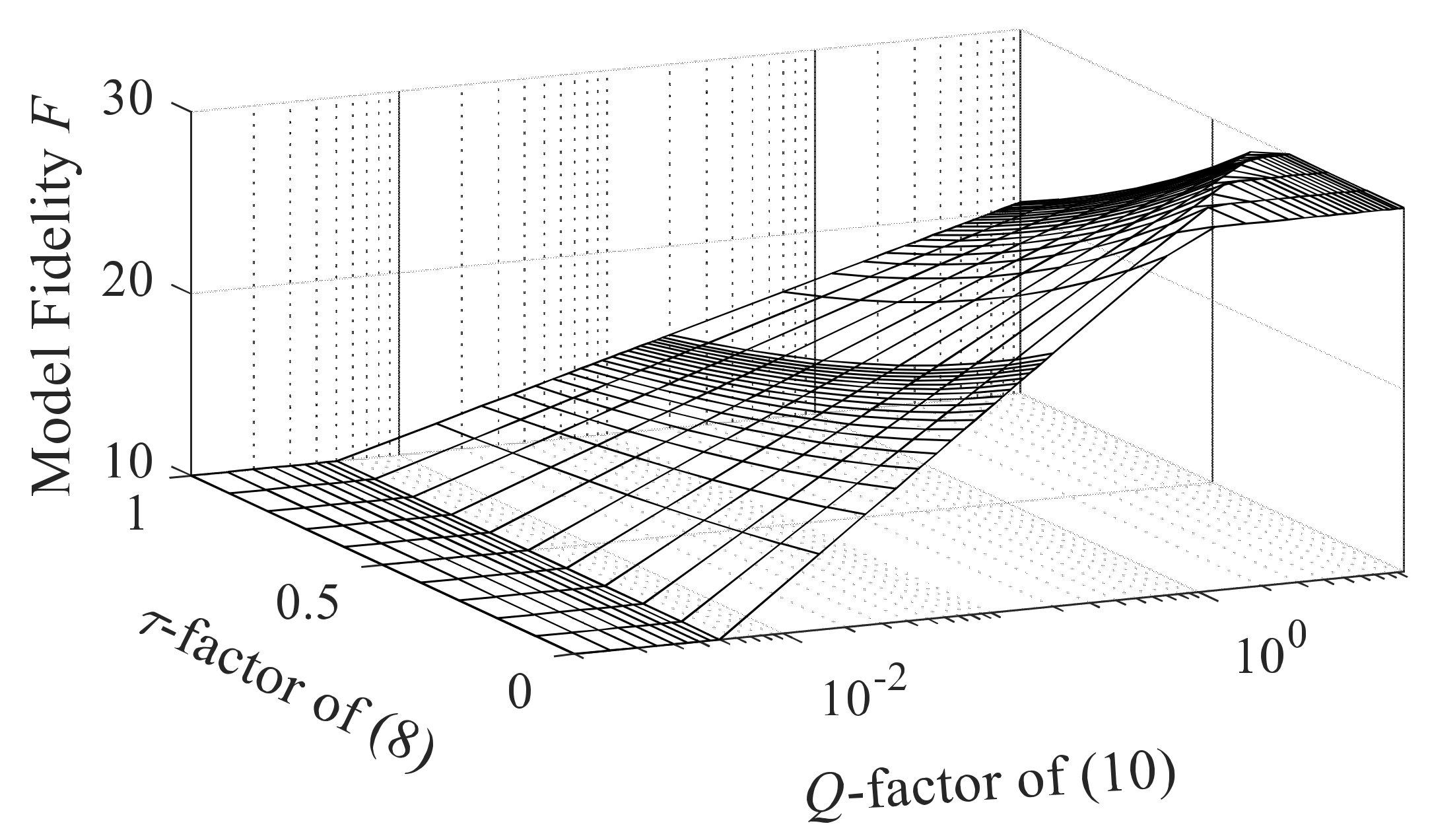
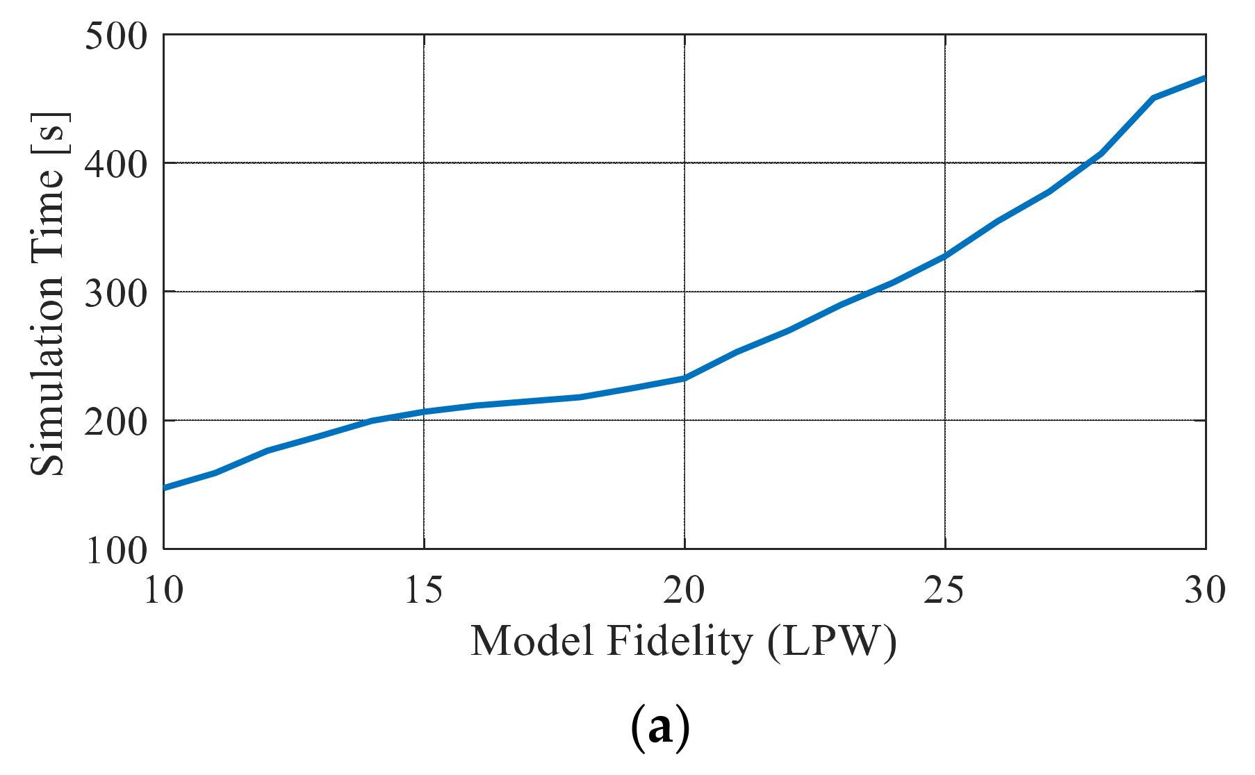
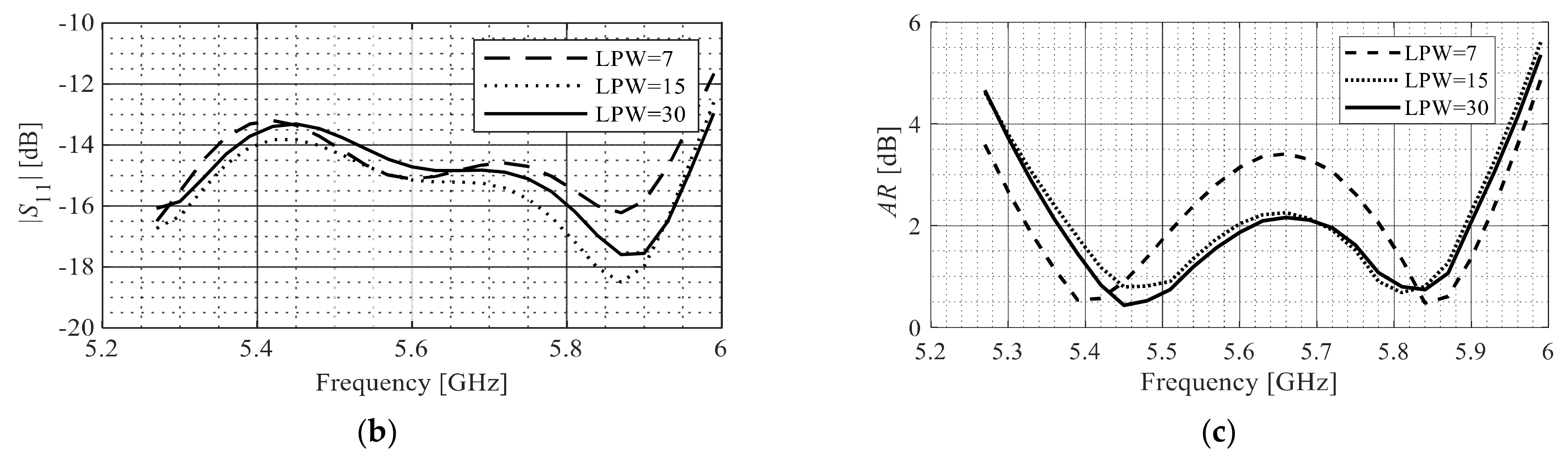
6.1. Variable-Fidelity EM Models

Figure 21 shows a circularly polarized (CP) patch antenna, as well as the dependence of the simulation time and model fidelity, adjusted using the parameter lines-per wavelength (LPW) in CST Microwave Studio, utilized to control the discretization density of the structure. It can be observed that reducing the number of mesh cells accelerates the simulation process, at the expense of accuracy degradation. For this particular antenna, the high-fidelity model is set up at LPW = 30 (simulation time 236 s), whereas the lowest-fidelity model, which still properly represents antenna characteristics, is set at LPW = 11 (simulation time 82 s). These two levels will be denoted as Fmax and Fmin, respectively.

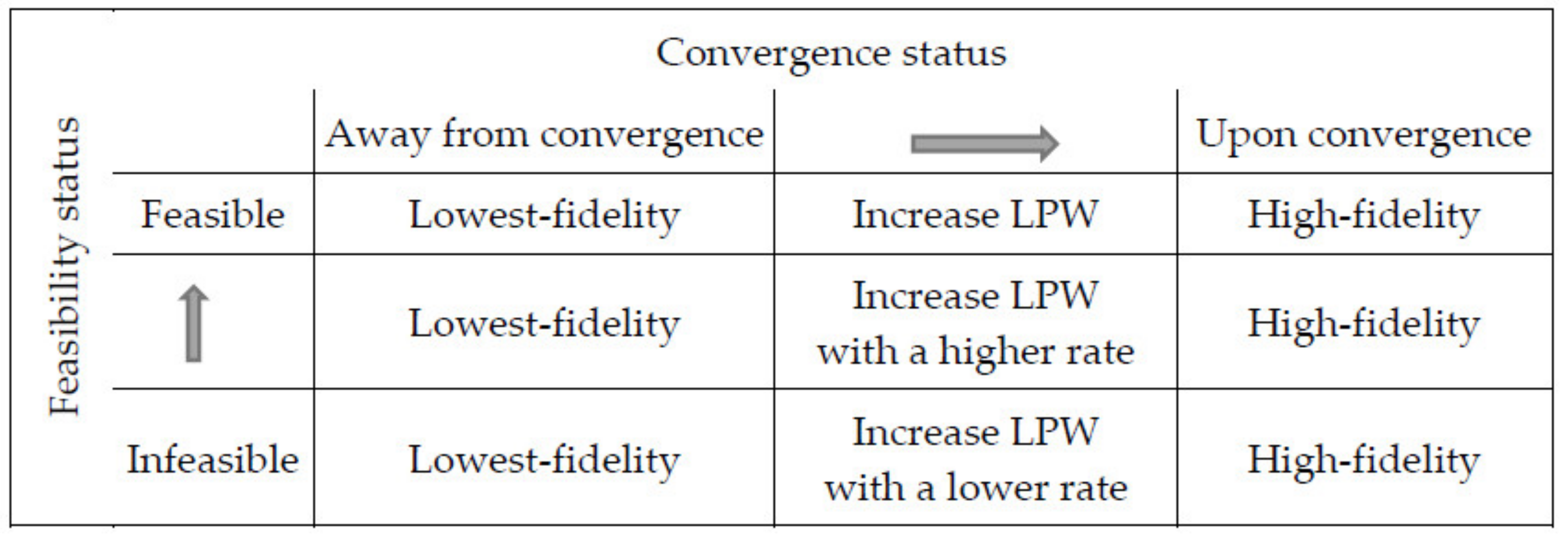
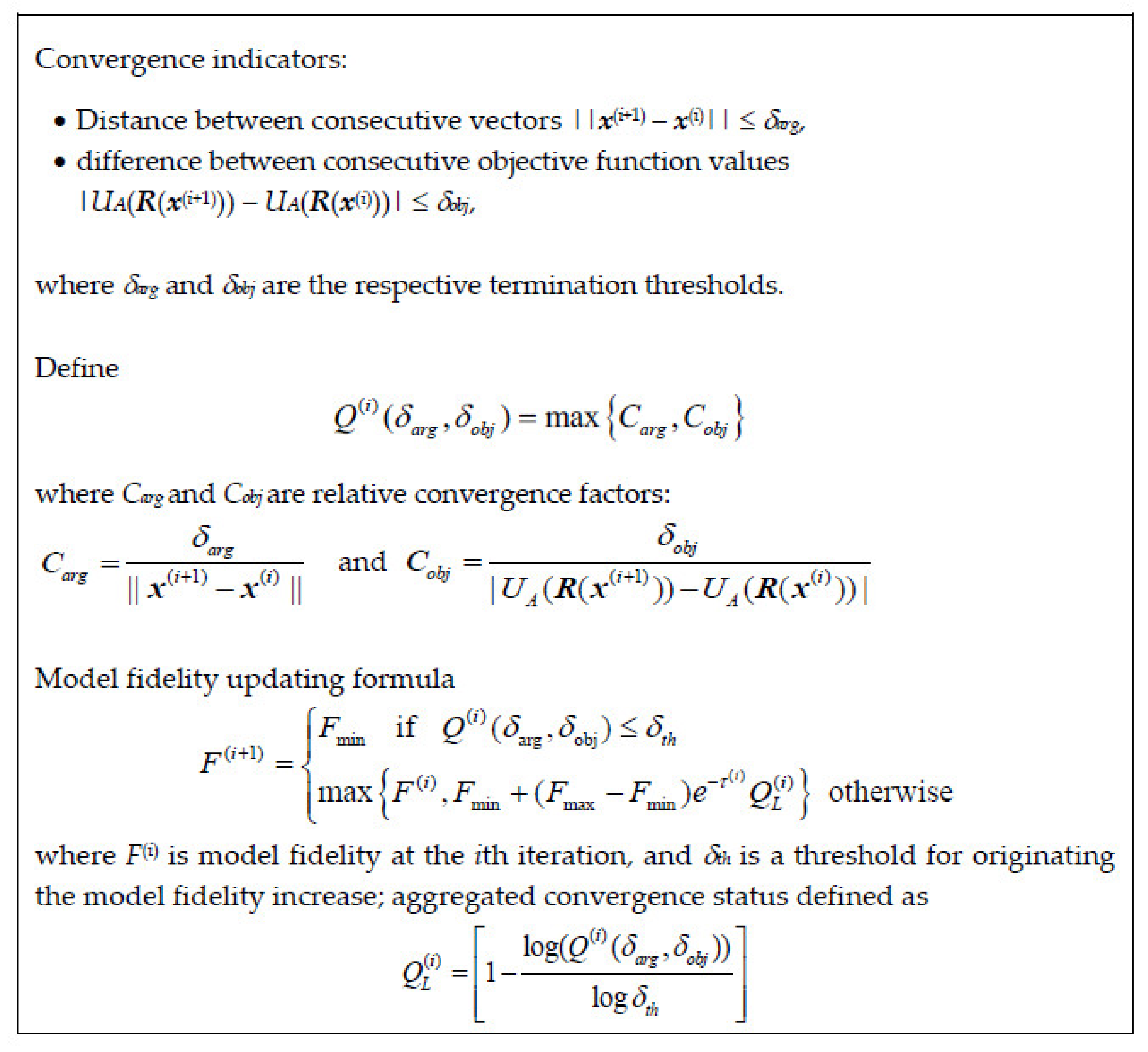
6.2. Model Management Scheme

The model management scheme of [46] adjusts the fidelity of the model, denoted as F, within the range Fmin ≤ F ≤ Fmax (cf. Section 6.1). The underlying optimization engine is the trust-region gradient-based algorithm [54]. Constraint control follows the adaptive scheme of [41], see also Section 3.2. The decision factors concerning the value of F have been shown in Figure 22. These can be summarized as follows:
  • The fidelity is set to Fmin early in the optimization process, regardless of the solution feasibility;
  • Fidelity is set to Fmax upon convergence for reliability reasons;
  • In the intermediate phase (i.e., either between infeasible and feasible, or when reaching convergence), the model fidelity depends on both the feasibility and the convergence status.
The feasibility status is defined as eτ(i), where τ(i) = max{j = 1, …, k: τj(i)} is the aggregated constraint violation at the ith iteration, where τj(i) = ζjcj. The normalization factors τcj are set to ensure that τj(i) = 1 when constraint violation gets close to a user-defined threshold (constraint-specific [46]). Here, the threshold is set to 2 dB for reflection-related constraints and 1 dB for axial-ratio-related ones. The convergence status has been explained in Figure 23, which also contains the model fidelity updating formula. The dependence between the simulation model fidelity and the convergence status and constraint violation is shown in Figure 24.

6.3. Illustration Example

Consider a circularly polarized patch antenna shown in Figure 25. The computational model setup has been described in Section 6.1. The goal is to reduce the antenna size subject to constraints listed in Figure 25b. The initial design has been obtained by minimizing the reflection response and axial ratio within the frequency band of interest (cf. Figure 26. The antenna has been optimized using the algorithm with adaptive adjustment of penalty factors [42], as well as the multi-fidelity procedure (also with adaptive penalty factors) described in this section.
The results shown in Table 6 demonstrate that the employment of variable resolution models considerably expedites the design process (by almost 50 percent), without being detrimental to the design quality. Furthermore, it enables excellent control of both design constraints.

7. Discussion and Conclusions

This paper presented an overview of the recent techniques for EM-driven size reduction in high-frequency structures. While simulation-based procedures, including numerical optimization, have been playing an increasing role in antenna and microwave design, miniaturization-oriented parameter tuning has been sparsely treated in the literature so far. In this work, we recalled the size reduction task along with its explicit and implicit formulations, as well as reviewed several recent methodologies developed to address its inherent challenges, specifically the need of controlling several performance figures and the presence of expensive constraints. The discussed procedures include implicit approaches with adaptive adjustment of penalty coefficients, an algorithm for a precise explicit constraint control, as well as a dedicated routine for optimization-based correction of equality constraint violation. Accelerated EM-driven miniaturization using variable-resolution models has been discussed as well. The juxtaposition of the discussed miniaturization frameworks is provided in Table 7. Theoretical considerations have been illustrated using a number of real-world examples of broadband and circular polarization antennas, we well as microstrip couplers.
The presented numerical results corroborate the efficacy of both implicit and explicit techniques, especially in terms of the precise control of the design constraints, but also achievable miniaturization rate. The former is instrumental in the appropriate identification of the minimum-size designs: as a reduction in physical dimensions is detrimental to electrical and field performance figures, constrained optima are normally allocated at the feasible region boundary. Consequently, the performance of the optimization process is contingent upon the ability to explore this region. The procedures presented in this paper make it possible while eliminating the need for meticulous tuning of the control parameters in conventional methods. As demonstrated, they can also be accelerated by employing variable-resolution computational models.
While the overall performance of the outlined methods is similar, implicit techniques (i.e., those featuring adaptive adjustment of penalty terms) are conceptually simpler and, therefore, easier to implement. Further, they generally ensure slightly better miniaturization rates, although the difference is minor. On the other hand, explicit methods offer more precise control over the design constraints. From the point of view of a potential user of the aforementioned frameworks, either of them may be considered an attractive alternative to conventional methods. For those reliant on experience-driven parametric studies, the outlined techniques may prove useful tools for achieving size reduction beyond any interactive approaches.
It should be reiterated that the primary purpose of the paper was to provide the reader with a number of alternatives in terms of possible algorithmic approaches for EM-driven size reduction, rather than to compare them against each other. As mentioned earlier, the overall performance of the presented algorithms is similar, whereas the major differences are concerned with the specific ways of handling constraints (which may be preferred for specific applications, as elaborated on in the paper) as well as due to implementation details and complexity.

Author Contributions

Conceptualization, A.P.-D. and S.K.; methodology, A.P.-D. and S.K.; software, A.P.-D. and M.M.; validation, A.P.-D. and S.K.; formal analysis, A.P.-D. and S.K.; investigation, A.P.-D.; resources, S.K.; data curation, A.P.-D. and M.M.; writing—original draft preparation, A.P.-D., M.M. and S.K.; writing—review and editing, A.P.-D. and S.K.; visualization, A.P.-D. and M.M.; supervision, S.K.; project administration, S.K.; funding acquisition, S.K. All authors have read and agreed to the published version of the manuscript.

Funding

This work was supported in part by the Icelandic Centre for Research (RANNIS) Grant 206606, and by Gdańsk University of Technology Grant DEC-41/2020/IDUB/I.3.3 under the Argentum Triggering Research Grants program—‘Excellence Initiative—Research University’.

Acknowledgments

The authors thank Dassault Systemes, France, for making CST Microwave Studio available.

Conflicts of Interest

The authors declare no conflict of interest. The funders had no role in the design of the study; in the collection, analyses, or interpretation of data; in the writing of the manuscript, or in the decision to publish the results.

References

  1. Wang, Z.; Kim, E.-S.; Liang, J.-G.; Kim, N.-Y. QFN-packaged bandpass filter with intertwined circular spiral inductor and integrated center-located capacitors using integrated passive device technology. IEEE Access 2019, 7, 13597–13607. [Google Scholar] [CrossRef]
  2. Yin, X.; Zhu, Z.; Liu, Y.; Lu, Q.; Liu, X.; Yang, Y. Ultra-compact TSV-based L-C low-pass filter with stopband up to 40 GHz for microwave applications. IEEE Trans. Microw. Theory. Tech. 2019, 67, 738–745. [Google Scholar] [CrossRef]
  3. Su, S.-W.; Lee, C.-T.; Hsiao, Y.-W. Compact two-inverted-F-antenna system with highly integrated π-shaped decoupling structure. IEEE Trans. Antennas Propag. 2019, 67, 6182–6186. [Google Scholar] [CrossRef]
  4. Byeon, C.W.; Park, C.S. Low-loss compact millimeter-wave power divider/combiner for phased array systems. IEEE Microw. Wirel. Compon. Lett. 2019, 29, 312–314. [Google Scholar] [CrossRef]
  5. Piekarz, I.; Sorocki, J.; Smolarz, R.; Gruszczynski, S.; Wincza, K. Four-node antenna feeding network for interfacing with differential front-end electronics. IEEE Access 2021, 9, 103728–103736. [Google Scholar] [CrossRef]
  6. Choudhary, D.K.; Chaudhary, R.K. Compact lowpass and dual-band bandpass filter with controllable transmission zero/center frequencies/passband bandwidth. IEEE Trans. Circuits Syst. II Exp. Briefs 2020, 67, 1044–1048. [Google Scholar] [CrossRef]
  7. Shen, G.; Che, W.; Xue, Q.; Yang, W. Characteristics of dual composite right/left-handed unit cell and its applications to bandpass filter design. IEEE Trans. Circuits Syst. II Exp. Briefs 2018, 65, 719–723. [Google Scholar] [CrossRef]
  8. Li, Z.; Wu, K.-L. Direct synthesis and design of wideband bandpass filter with composite series and shunt resonators. IEEE Trans. Microw. Theory Tech. 2017, 65, 3789–3800. [Google Scholar] [CrossRef]
  9. Chi, J.-G.; Kom, Y.-J. A compact wideband millimeter-wave quadrature hybrid coupler using artificial transmission lines on a glass substrate. IEEE Microw. Wirel. Compon. Lett. 2020, 30, 1037–1040. [Google Scholar] [CrossRef]
  10. Kim, D.-M.; Min, B.-W.; Yook, J.-M. Compact mm-wave bandpass filters using silicon integrated passive device technology. IEEE Microw. Wirel. Compon. Lett. 2019, 29, 638–640. [Google Scholar] [CrossRef]
  11. Hagag, M.F.; Abu Khater, M.; Sinanis, M.D.; Peroulis, D. Ultra-compact tunable filtering rat-race coupler based on a half-mode SIW evanescent-mode cavity resonator. IEEE Trans. Microw. Theory Tech. 2018, 66, 5563–5572. [Google Scholar] [CrossRef]
  12. Hagag, M.F.; Peroulis, D. A compact tunable filtering rat-race coupler. In Proceedings of the 2018 IEEE/MTT-S International Microwave Symposium-IMS, Philadephia, PA, USA, 10–15 June 2018; pp. 1118–1121. [Google Scholar]
  13. Lin, Y.-S.; Liu, Y.-R.; Chan, C.-H. Novel miniature dual-band rat-race coupler with arbitrary power division ratios using differential bridged-T coils. IEEE Trans. Microw. Theory Tech. 2021, 69, 590–602. [Google Scholar] [CrossRef]
  14. Liu, Y.-R.; Chan, C.-H.; Lin, Y.-S. Miniature wideband rat-race coupler in silicon-based integrated passive device technology. In Proceedings of the 2020 IEEE/MTT-S International Microwave Symposium (IMS), Loas Angeles, CA, USA, 4–6 August 2020; pp. 727–730. [Google Scholar]
  15. Koziel, S.; Pietrenko Dabrowska, A. Performance-based nested surrogate modeling of antenna input characteristics. IEEE Trans. Antennas Propag. 2019, 67, 2904–2912. [Google Scholar] [CrossRef]
  16. Song, Y.; Cheng, Q.S.; Koziel, S. Multi-fidelity local surrogate model for computationally efficient microwave component design optimization. Sensors 2019, 19, 3023. [Google Scholar] [CrossRef] [PubMed]
  17. Koziel, S.; Pietrenko Dabrowska, A. Design-oriented modeling of antenna structures by means of two-level kriging with explicit dimensionality reduction. AEU-Int. J. Electron. Comm. 2020, 127, 153466. [Google Scholar] [CrossRef]
  18. Pietrenko-Dabrowska, A.; Koziel, S. Antenna modeling using variable-fidelity EM simulations and constrained co-kriging. IEEE Access 2020, 8, 91048–91056. [Google Scholar] [CrossRef]
  19. Pietrenko-Dabrowska, A.; Koziel, S. Surrogate modeling of impedance matching transformers by means of variable-fidelity EM simulations and nested co-kriging. Int. J. RF Microw. Comput. Aided Eng. 2020, 30, e22268. [Google Scholar] [CrossRef]
  20. Koziel, S.; Pietrenko Dabrowska, A. Low-cost performance-driven modelling of compact microwave components with two-layer surrogates and gradient kriging. AEU Int. J. Electron. Comm. 2020, 126, 153419. [Google Scholar] [CrossRef]
  21. Koziel, S.; Pietrenko Dabrowska, A. Reliable data-driven modeling of high-frequency structures by means of nested kriging with enhanced design of experiments. Eng. Comput. 2019, 36, 2293–2308. [Google Scholar] [CrossRef]
  22. Koziel, S.; Pietrenko Dabrowska, A. Reduced-cost design closure of antennas by means of gradient search with restricted sensitivity updates. Metrol. Meas. Syst. 2019, 26, 595–605. [Google Scholar]
  23. Pietrenko-Dabrowska, A.; Koziel, S. Expedited antenna optimization with numerical derivatives and gradient change tracking. Eng. Comput. 2019, 37, 1179–1193. [Google Scholar] [CrossRef]
  24. Pietrenko-Dabrowska, A. Rapid tolerance-aware design of miniaturized microwave passives by means of confined-domain surrogates. Int. J. Num. Model. 2020, 33, e2779. [Google Scholar]
  25. Koziel, S.; Pietrenko-Dabrowska, A. Efficient gradient-based algorithm with numerical derivatives for expedited optimization of multi-parameter miniaturized impedance matching transformers. Radioengineering 2019, 27, 572–578. [Google Scholar] [CrossRef]
  26. Koziel, S.; Pietrenko-Dabrowska, A. An efficient trust-region algorithm for wideband antenna optimization. In Proceedings of the 2019 13th European Conference on Antennas and Propagation (EuCAP), Cracow, Poland, 31 March–5 April 2019; pp. 1–5. [Google Scholar]
  27. Pietrenko-Dabrowska, A.; Koziel, S. Expedited gradient-based design closure of antennas using variable-resolution simulations and sparse sensitivity updates. IEEE Trans. Antennas Propag. 2021, 70, 4925–4930. [Google Scholar] [CrossRef]
  28. Koziel, S.; Pietrenko Dabrowska, A. Fast multi-objective optimization of antenna structures by means of data-driven surrogates and dimensionality reduction. IEEE Access 2020, 8, 183300–183311. [Google Scholar] [CrossRef]
  29. Pietrenko-Dabrowska, A.; Koziel, S. Accelerated multiobjective design of miniaturized microwave components by means of nested kriging surrogates. Int. J. RF Microw. Comput. Aided Eng. 2020, 30, e22124. [Google Scholar] [CrossRef]
  30. Koziel, S.; Pietrenko-Dabrowska, A. Constrained multi-objective optimization of compact microwave circuits by design triangulation and pareto front interpolation. Eur. J. Oper. Res. 2022, 299, 302–312. [Google Scholar] [CrossRef]
  31. Liu, B.; Yang, H.; Lancaster, M.J. Global optimization of microwave filters based on a surrogate model-assisted evolutionary algorithm. IEEE Trans. Microw. Theory Tech. 2017, 65, 1976–1985. [Google Scholar] [CrossRef]
  32. Lalbakhsh, A.; Afzal, M.U.; Esselle, K.P. Multiobjective particle swarm optimization to design a time-delay equalizer metasurface for an electromagnetic band-gap resonator antenna. IEEE Antennas Wirel. Propag. Lett. 2017, 16, 912–915. [Google Scholar] [CrossRef]
  33. Tomasson, J.A.; Koziel, S.; Pietrenko Dabrowska, A. Quasi-global optimization of antenna structures using principal components and affine subspace-spanned surrogates. IEEE Access 2020, 8, 50078–50084. [Google Scholar] [CrossRef]
  34. Kaur, M.; Sivia, J.S. Giuseppe Peano and Cantor set fractals based miniaturized hybrid fractal antenna for biomedical applications using artificial neural network and firefly algorithm. Int. J. RF Microw. CAE 2020, 30, e22000. [Google Scholar] [CrossRef]
  35. Dhakshinamoorthi, M.K.; Gokulakkrizhna, S.; Denesh Kumar, M.; Subha, M.; Mekaladevi, V. Rectangular microstrip patch antenna miniaturization using improvised genetic algorithm. In Proceedings of the 2020 4th International Conference on Trends in Electronics and Informatics (ICOEI), Tirunelveli, India, 15–17 June 2020; pp. 894–898. [Google Scholar]
  36. Boudjerda, M.; Reddaf, A.; Kacha, A.; Hamdi-Cherif, K.; Alharbi, T.E.A.; Alzaidi, M.S.; Alsharef, M.; Ghoneim, S.S.M. Design and optimization of miniaturized microstrip patch antennas using a genetic algorithm. Electronics 2022, 11, 2123. [Google Scholar] [CrossRef]
  37. Lamsalli, M.; El Hamichi, A.; Boussouis, M.; Touhami, N.A.; Elhamadi, T. Genetic algorithm optimization for microstrip patch antenna miniaturization. Progr. Electr. Res. Lett. 2016, 60, 113–120. [Google Scholar] [CrossRef]
  38. Souza, E.A.M.; Oliveira, P.S.; D’Assunção, A.G.; Mendonça, L.M.; Peixeiro, C. Miniaturization of a microstrip patch antenna with a Koch fractal contour using a social spider algorithm to optimize shorting post position and inset feeding. Int. J. Antennas Propag. 2019, 2019, 6284830. [Google Scholar] [CrossRef]
  39. Johanesson, D.O.; Koziel, S. Feasible space boundary search for improved optimization-based miniaturization of antenna structures. IEEE Microw. Antennas Propag. 2018, 12, 1273–1278. [Google Scholar] [CrossRef]
  40. Mahrokh, M.; Koziel, S. Optimization-based antenna miniaturization using adaptively adjusted penalty factors. Electronics 2021, 10, 1751. [Google Scholar] [CrossRef]
  41. Mahrokh, M.; Koziel, S. Explicit size-reduction of circularly polarized antennas through constrained optimization with penalty factor adjustment. IEEE Access 2021, 9, 132390–132396. [Google Scholar] [CrossRef]
  42. Koziel, S.; Pietrenko Dabrowska, A. Reliable EM-driven size reduction of antenna structures by means of adaptive penalty factors. IEEE Trans. Antennas Propag. 2022, 70, 1389–1401. [Google Scholar] [CrossRef]
  43. Koziel, S.; Pietrenko Dabrowska, A. Direct constraint control for EM-based miniaturization of microwave passives. Sci. Rep. 2022, 12, 13320. [Google Scholar] [CrossRef]
  44. Pietrenko-Dabrowska, A.; Koziel, S. On EM-driven size reduction of antenna structures with explicit constraint handling. IEEE Access 2021, 9, 165766–165772. [Google Scholar] [CrossRef]
  45. Koziel, S.; Pietrenko Dabrowska, A.; Mahrokh, M. On decision-making strategies for improved-reliability size reduction of microwave passives: Intermittent correction of equality constraints and adaptive handling of inequality constraints. Knowl.-Based Syst. 2022, 255, 109745. [Google Scholar] [CrossRef]
  46. Mahrokh, M.; Koziel, S. Improved-efficacy EM-based antenna miniaturization by multi-fidelity simulations and objective function adaptation. Energies 2021, 15, 403. [Google Scholar] [CrossRef]
  47. Tan, X.; Sun, J.; Lin, F. A compact frequency-reconfigurable rat-race coupler. IEEE Microw. Wirel. Comp. Lett. 2020, 30, 665–668. [Google Scholar] [CrossRef]
  48. Chi, P.-L.; Shang, S.-A.; Yang, T. Novel compact coupler with tunable frequency, phase difference, and power-dividing ratio. IEEE Microw. Wirel. Comp. Lett. 2021, 31, 1119–1122. [Google Scholar] [CrossRef]
  49. Zhu, Y.; Dong, Y. A novel compact wide-stopband filter with hybrid structure by combining SIW and microstrip technologies. IEEE Microw. Wirel. Comp. Lett. 2021, 31, 841–844. [Google Scholar] [CrossRef]
  50. Wen, L.; Gao, S.; Sanz-Izquierdo, B.; Wang, C.; Hu, W.; Ren, X.; Wu, J. Compact and wideband crossed dipole antenna using coupling stub for circular polarization. IEEE Trans. Antennas Propag. 2022, 70, 27–34. [Google Scholar] [CrossRef]
  51. Sun, L.; Li, Y.; Zhang, Z. Wideband dual-polarized endfire antenna based on compact open-ended cavity for 5G Mm-Wave mobile phones. IEEE Trans. Antennas Propag. 2022, 70, 1632–1642. [Google Scholar] [CrossRef]
  52. Neophytou, K.; Steeg, M.; Stöhr, A.; Antoniades, M.A. Compact folded leaky-wave antenna radiating a fixed beam at broadside for 5G mm-Wave applications. IEEE Antennas Wireless Propag. Lett. 2022, 21, 292–296. [Google Scholar] [CrossRef]
  53. Ye, M.; Li, X.; Chu, Q. Single-layer circularly polarized antenna with fan-beam endfire radiation. IEEE Ant. Wirel. Propag. Lett. 2017, 16, 20–23. [Google Scholar] [CrossRef]
  54. Conn, A.R.; Gould, N.I.M.; Toint, P.L. Trust Region Methods; SIAM: Philadelphia, PA, USA, 2000. [Google Scholar]
  55. Alsath, M.G.N.; Kanagasabai, M. Compact UWB monopole antenna for automotive communications. IEEE Trans. Ant. Prop. 2015, 63, 4204–4208. [Google Scholar] [CrossRef]
  56. Kumar, B.P.; Kumar, C.; Guha, D. A new design approach to improve the circular polarization characteristics of a microstrip antenna. In Proceedings of the 2018 IEEE Indian Conference on Antennas and Propogation (InCAP), Hyderabad, India, 16–19 December 2018; pp. 1–2. [Google Scholar]
  57. Haq, M.A.; Koziel, S. Simulation-based optimization for rigorous assessment of ground plane modifications in compact UWB antenna design. Int. J. RF Microw. CAE 2018, 28, e21204. [Google Scholar] [CrossRef]
  58. Phani Kumar, K.V.; Karthikeyan, S.S. A novel design of rat-race coupler using defected microstrip structure and folding technique. In Proceedings of the 2013 IEEE Applied Electromagnetics Conference (AEMC), Bhubaneswar, India, 18–20 December 2013; pp. 1–2. [Google Scholar]
  59. Letavin, D.A.; Shabunin, S.N. Miniaturization of a branch-line coupler using microstrip cells. In Proceedings of the 2018 XIV International Scientific-Technical Conference on Actual Problems of Electronics Instrument Engineering (APEIE), Novosibirsk, Russia, 2–6 October 2018; pp. 62–65. [Google Scholar]
  60. Letavin, D.A.; Mitelman, Y.E.; Chechetkin, V.A. Compact microstrip branch-line coupler with unequal power division. In Proceedings of the 2017 11th European Conference on Antennas and Propagation (EUCAP), Paris, France, 19–24 March 2017; pp. 1162–1165. [Google Scholar]
  61. Malekabadi, S.A.; Attari, A.R.; Mirsalehi, M.M. Compact broadband circular polarized microstrip antenna with wideband axial-ratio bandwidth. In Proceedings of the 2008 International Symposium on Telecommunications, Tehran, Iran, 27–28 August 2008; pp. 106–109. [Google Scholar]
Figure 1. Adaptive constraint violation adjustment according to the methodology of [42].
Energies 15 06955 g001
Figure 2. Penalty coefficient setup according to the methodology of [42].
Energies 15 06955 g002
Figure 3. Ultrawideband antenna [55]: (a) geometry, (b) essential parameters.
Energies 15 06955 g003
Figure 4. Representative run of the algorithm [42] optimizing the antenna of Figure 3: (a) antenna reflection characteristics at the initial (- - -) and optimized design (—), horizontal line marks design specifications; (b) evolution of penalty factor value across optimization course.
Energies 15 06955 g004
Figure 5. Rules for penalty coefficient adjustment in the methodology of [41].
Energies 15 06955 g005
Figure 6. Circular patch antenna [56]: (a) geometry, (b) essential parameters.
Energies 15 06955 g006
Figure 7. Size reduction in the antenna of Figure 6 using algorithm [41]: (a,b) reflection S11 and axial ratio AR, respectively, at the initial (- - -) and optimized design (—), horizontal lines mark design specifications; (c,d) evolution of the penalty factors corresponding to S11 and AR, respectively, throughout optimization process.
Energies 15 06955 g007
Figure 8. Updating the trust-region size according to the methodology of [44].
Energies 15 06955 g008
Figure 9. Rules for computing gain ratios ρk [44].
Energies 15 06955 g009
Figure 10. Prediction of constraints with the use of linear model SL.ineq.k.: (top) design shift from x(i) to x(i+1) as a result of solving (6), the purpose of the design relocation is to minimize the footprint area and to meet the constraint (as predicted by SL.ineq.k); (bottom-left) satisfactory prediction of a linear model; (bottom-right) poor prediction and infeasible new design (as assessed by the true constraint value rendered by EM analysis), so, d(i) is to be reduced in the next iteration.
Energies 15 06955 g010
Figure 11. Broadband antenna [57]: (a) geometry, (b) essential parameters.
Energies 15 06955 g011
Figure 12. Representative run of the algorithm [44] optimizing the antenna of Figure 11: (a) antenna reflection characteristics at the initial (- - -) and optimized design (—), (b) evolution of antenna size, (c) evolution of constraint violation.
Energies 15 06955 g012
Figure 13. Rat-race coupler [58]: (a) geometry, (b) essential parameters.
Energies 15 06955 g013
Figure 14. Initial (gray) and optimized (black) S-parameters of the circuit of Figure 13. The vertical and horizontal lines mark the target operating bandwidth and the acceptance level for the matching |S11| and isolation |S41| responses. Additionally, shown is the evolution of the circuit size and constraint violations (in case of feasibility, violations shown as zero): (a) design scenario I (bandwidth 1.15 GHz to 1.25 GHz), (b) design scenario II (bandwidth 1.18 GHz to 1.22 GHz).
Energies 15 06955 g014
Figure 15. Design relocation from feasible region boundary for inequality and equality constraints: (a) inequality constraint: the designs produced from the current design x(i) may be located in either feasible or infeasible region, (b) equality constraint: essentially all designs produced from x(i) are infeasible due to feasible region being a thin set. Consequently, exploration of the feasible space is more difficult for the equality constraints than the inequality ones.
Energies 15 06955 g015
Figure 16. Correction of equality constraints according to the methodology presented in [45].
Energies 15 06955 g016
Figure 17. Optimization-based correction scheme for efficient control of equality constraints: (a) the concept: design x(i+1) obtained in the ith iteration of the optimization algorithm, starting from x(i), is infeasible; it is brought closer to a feasible space using the correction procedure [29], without neither degrading inequality constraints nor the circuit area; the corrected design xc(i+1) features reduced equality constraint values Seq.k(xc(i+1)) < Seq.k(x(i+1)), k = 1, …, neq, as well as A(xc(i+1)) ≤ A(x(i+1)), and Sineq.j(xc(i+1)) ≤ Sineq.j(x(i+1)), j = 1, …, nineq, (b) graphical illustration of the intermittent equality constraint correction throughout the optimization run.
Energies 15 06955 g017
Figure 18. Demonstration case studies for equality constraint correction methodology of [45]: (a) branch-line coupler geometry (Circuit I) [59], (b) branch-line coupler geometry (Circuit II) [60], (c) essential circuit parameters.
Energies 15 06955 g018
Figure 19. Initial (gray) and optimized (black) S-parameters of Circuit I. The vertical and horizontal lines mark the target operating bandwidth and the acceptance level for the matching |S11| and isolation |S41| responses. Additionally, shown is the evolution of the circuit size and constraint violations (in case of feasibility, violations shown as zero), as well as evolution of the penalty coefficient for the inequality constraint. The vertical line shows the target operating frequency of 1.0 GHz.
Energies 15 06955 g019
Figure 20. Initial (gray) and optimized (black) S-parameters of Circuit II. The vertical and horizontal lines mark the target operating bandwidth and the acceptance level for the matching |S11| and isolation |S41| responses. Additionally, shown is the evolution of the circuit size and constraint violations (in case of feasibility, violations shown as zero), as well as evolution of the penalty coefficient for the inequality constraint. The vertical line shows the target operating frequency of 2.0 GHz.
Energies 15 06955 g020aEnergies 15 06955 g020b
Figure 21. CP antenna (geometry shown in Figure 25) (a); EM responses for various model fidelities: (a) dependence of the simulation time on the model discretization density, (b) reflection responses and (c) axial ratio for various fidelity levels.
Energies 15 06955 g021aEnergies 15 06955 g021b
Figure 22. Decision factors for model fidelity adjustment proposed in [46]. The fidelity control depends on the solution feasibility as well as the convergence status of the optimization process.
Energies 15 06955 g022
Figure 23. Definition of the convergence status and the model fidelity updating formula.
Energies 15 06955 g023
Figure 24. Dependence between the simulation model fidelity and the convergence status Q, as well as aggregated constraint violation τ. The dependence is monotonic with respect to both control factors except from the early stages of the algorithm and when close to convergence. The plot created for exemplary model resolution levels Fmin = 10, Fmax = 30, assuming δth = 5 × 10⁻³.
Energies 15 06955 g024
Figure 25. Circular-polarization patch antenna [61]: (a) geometry, (b) essential parameters.
Energies 15 06955 g025
Figure 26. Results for Antenna of Figure 25 using the algorithm [46] incorporating multi-fidelity model management and adaptive penalty coefficients: (a) reflection responses, (b) axial ratio responses, (c) evolution of the model fidelity. The horizontal lines represent the design specifications.
Energies 15 06955 g026
Table 1. Optimization results for antenna of Figure 3.
Optimization ApproachPerformance Figure
Antenna
Footprint A [mm2] 1
Std(A) 2Constraint
Violation D [dB] 3
Std(D) [dB] 4
Penalty function approachβ = 102113.79.078.400.53
β = 103250.424.01.200.50
β = 104318.660.00.140.10
β = 105331.663.40.100.14
β = 106367.651.90.050.11
Adaptive penalty factors [28]281.637.10.230.15
1 Optimized antenna footprint averaged over ten algorithm runs. 2 Standard deviation of the antenna footprint averaged over ten algorithm runs. 3 Average constraint violation D = {3.1 GHz ≤ f ≤ 10.6 GHz: max|S11(f)|} + 10 dB. 4 Standard deviation of the constraint violation D, averaged over ten algorithm runs.
Table 2. Optimization results for antenna of Figure 6.
Algorithm with
Fixed Penalty Factors
Antenna
Footprint A [mm2] 1
Constraint
Violation
ζS11 [dB] 2
Constraint
Violation
ζAR [dB] 3
βARβS11
10102374.382.770
10103323.372.240.2
10104334.372.690.01
10105340.242.150.01
102102309.990.053.8
102103361.730.330
102104359.710.270
102105356.180.200
103102404.580.070
103103421.750.050
103104421.750.050
103105421.750.050
104102455.410.030
104103455.410.030
104104455.410.030
104105455.410.030
Adaptive penalty factors [41]373.3600
1 Optimized antenna footprint. 2 Constraint violation ζS11 = {8.1 GHz ≤ f ≤ 8.3 GHz: max|S11(f)|} + 10 dB. 3 Constraint violation ζAR = {8.1 GHz ≤ f ≤ 8.3 GHz: max|AR(f)|} + 3 dB.
Table 3. Optimization results for antenna of Figure 11.
Optimization ApproachPerformance Figure
Antenna Footprint A [mm2] 1Std(A) 2Constraint Violation
D [dB] 3
Std(D)
[dB] 4
Penalty function approachβ = 10256.13.88.60.60
β = 103212.814.31.00.40
β = 104255.025.10.150.10
β = 105280.147.40.050.07
β = 106285.829.60.000.01
Adaptive penalty
factors [28]
215.63.60.250.14
Explicit constraint handling [30]224.46.70.100.21
1 Optimized antenna footprint averaged over ten algorithm runs. 2 Standard deviation of the antenna footprint averaged over ten algorithm runs. 3 Average constraint violation D = {3.1 GHz ≤ f ≤ 10.6 GHz: max|S11(f)|} + 10 dB. 4 Standard deviation of the constraint violation D, averaged over ten algorithm runs.
Table 4. Optimization results for the circuit of Figure 13.
Optimization ApproachPerformance Parameters
Design Scenario I
(F = [1.15 1.25] GHz)
Design Scenario II
(F = [1.18 1.22] GHz)
MethodSetupFootprint Area A [mm2] 1Violation of
Equality
Constraint
g1 [dB] 2
Violation of Inequality Constraint g2 [dB] 3Footprint Area A [mm2] 1Violation of Equality Constraint
g1 [dB] 3
Violation of Inequality Constraint g2 [dB] 4
Implicit constraint handling
(penalty function approach)
β1 = 101, β2 = 10110670.170.710430.12−0.7
β1 = 101, β2 = 1026810.0110.46790.009.4
β1 = 101, β2 = 10310630.030.110630.03−1.0
β1 = 101, β2 = 10410970.02−0.110970.02−1.2
β1 = 102, β2 = 10111200.040.611200.04−0.5
β1 = 102, β2 = 10211340.00−0.311340.00−1.7
β1 = 102, β2 = 10311330.000.111330.00−1.2
β1 = 102, β2 = 10410380.031.110380.030.0
β1 = 103, β2 = 10111650.05−0.311650.05−1.7
β1 = 103, β2 = 10211190.01−0.111190.01−1.3
β1 = 103, β2 = 10311520.06−0.311520.06−1.6
β1 = 103, β2 = 10411170.08−0.110470.08−1.7
β1 = 104, β2 = 10112180.00−0.011360.020.2
β1 = 104, β2 = 10212080.00−0.211320.01−2.1
β1 = 104, β2 = 10311520.00−0.511520.00−1.7
β1 = 104, β2 = 10411520.02−0.111340.00−2.2
Explicit constraint
handling [43]
11060.04−0.110450.01−0.1
1 Optimized antenna footprint. 2 Constraint violation g1 = ||S31(x, f0) − S21(x, f0)|| − 0.1 dB; f0 = 1.2 GHz. 3 Constraint violation g2 = max{fF: max{|S11(x, f)|, |S41(x, f)|}} + 20 dB; f0 = 1.2 GHz, F = 100 Mhz. 4 Constraint violation g1 = ||S31(x, f0) − S21(x, f0)|| − 0.1 dB; f0 = 1.2 GHz. 5 Constraint violation g2 = max{fF: max{|S11(x,f)|, |S41(x,f)|}} + 20 dB; f0 = 1.2 GHz, F = 40 Mhz.
Table 5. Optimization results for Circuit I and Circuit II of Figure 18.
Optimization ApproachPerformance Parameters
Circuit I (f0 = 1.0 GHz)Circuit II (f0 = 2.0 GHz)
MethodSetupFootprint
Area
A [mm2] 1
Violation
of Equality Constraint
g1 [dB] 2
Violation
of Inequality Constraint
g2 [dB] 3
Footprint
Area
A [mm2] 1
Violation
of Equality Constraint
g3 [dB] 4
Violation
of Inequality Constraint
g4 [dB] 5
Implicit constraint handling
(penalty function approach)
β1 = 101, β2 = 101730.0113.81300.032.1
β1 = 101, β2 = 102750.0113.81350.061.8
β1 = 101, β2 = 1033051.122.31211.750.3
β1 = 101, β2 = 1043341.220.21460.020.1
β1 = 102, β2 = 101730.0113.81140.024.7
β1 = 102, β2 = 102730.0113.81410.042.9
β1 = 102, β2 = 1033820.202.41350.010.5
β1 = 102, β2 = 1044280.080.11520.010.1
β1 = 103, β2 = 101730.0113.81410.001.1
β1 = 103, β2 = 1022680.0311.51400.091.2
β1 = 103, β2 = 1033240.073.71420.021.3
β1 = 103, β2 = 1044140.040.21480.010.2
β1 = 104, β2 = 1012620.0011.71640.001.3
β1 = 104, β2 = 1023030.009.62000.006.1
β1 = 104, β2 = 1034480.000.02030.015.0
β1 = 104, β2 = 1044190.010.32070.010.3
Optimization-based equality constraint correction [44]3620.030.21290.030.4
1 Optimized antenna footprint. 2 Constraint violation g1 = ||S31(x, f0) − S21(x,f0)||; f0 = 1.0 GHz. 3 Constraint violation g2 = max{|S11(x, f0)|, |S41(x, f0)|} + 20 dB; f0 = 1.0 GHz. 4 Constraint violation g3 = ||S31(x,f0) − S21(x,f0)||; f0 = 2.0 GHz. 5 Constraint violation g4 = max{|S11(x, f0)|, |S41(x, f0)|} + 20 dB; f0 = 2.0 GHz.
Table 6. Optimization results for antenna of Figure 25.
Performance FiguresOptimization Method
Adaptive Penalty Factors [42]Variable-Fidelity 4
EM Simulations + Adaptive Penalty Factors [46]
Area A [mm2] 1372.7368
First constraint violation ζS11 [dB] 200.02
Second constraint violation ζAR [dB] 300
CPU timeAbsolute [h]8.84.7
Relative to Rf13572
Saving [%]47
1 Optimized antenna footprint. 2 Constraint violation ζS11 = {5.36 GHz ≤ f ≤ 5.9 GHz: max|S11(f)|} + 10. 3 Constraint violation ζAR = {5.36 GHz ≤ f ≤ 5.9 GHz: max|AR(f)|} + 3. 4 Simulation model fidelity set using LPW parameter of CST Microwave Studio that controls structure density discretization.
Table 7. Main features of the considered miniaturization algorithms.
ApproachImplicit Constraint Handling
with Adaptive Penalty Factors
(Section 3)
Explicit
Constraint
Handling
(Section 4)
Equality
Constraint Control through
Optimization-Based Correction
(Section 5)
Expedited
Optimization-Based
Miniaturization Algorithm
(Section 6)
VersionsConvergence-based penalty factor adjustment
(Section 3.1)
Penalty factor adjustment based on constraint violation improvement
(Section 3.2)
Constraint treatmentEqualityImplicitImplicitExplicitExplicitImplicit
InequalityImplicitImplicitExplicitImplicitImplicit
Simulation modelHigh-fidelityHigh-fidelityHigh-fidelityHigh-fidelityVariable-fidelity
Publisher’s Note: MDPI stays neutral with regard to jurisdictional claims in published maps and institutional affiliations.

