Offshore Wind Power Forecasting—A New Hyperparameter Optimisation Algorithm for Deep Learning Models

Abstract

The main obstacle against the penetration of wind power into the power grid is its high variability in terms of wind speed fluctuations. Accurate power forecasting, while making maintenance more efficient, leads to the profit maximisation of power traders, whether for a wind turbine or a wind farm. Machine learning (ML) models are recognised as an accurate and fast method of wind power prediction, but their accuracy depends on the selection of the correct hyperparameters. The incorrect choice of hyperparameters will make it impossible to extract the maximum performance of the ML models, which is attributed to the weakness of the forecasting models. This paper uses a novel optimisation algorithm to tune the long short-term memory (LSTM) model for short-term wind power forecasting. The proposed method improves the power prediction accuracy and accelerates the optimisation process. Historical power data of an offshore wind turbine in Scotland is utilised to validate the proposed method and compare its outcome with regular ML models tuned by grid search. The results revealed the significant effect of the optimisation algorithm on the forecasting models’ performance, with improvements of the RMSE of 7.89, 5.9, and 2.65 percent, compared to the persistence and conventional grid search-tuned Auto-Regressive Integrated Moving Average (ARIMA) and LSTM models.

1. Introduction

Undoubtedly, to accelerate economic growth, power production through renewable energy sources needs to increase because conventional methods such as using fossil fuels have irreparable consequences, including pollution, climate change, and the depletion of the ozone layer [1].

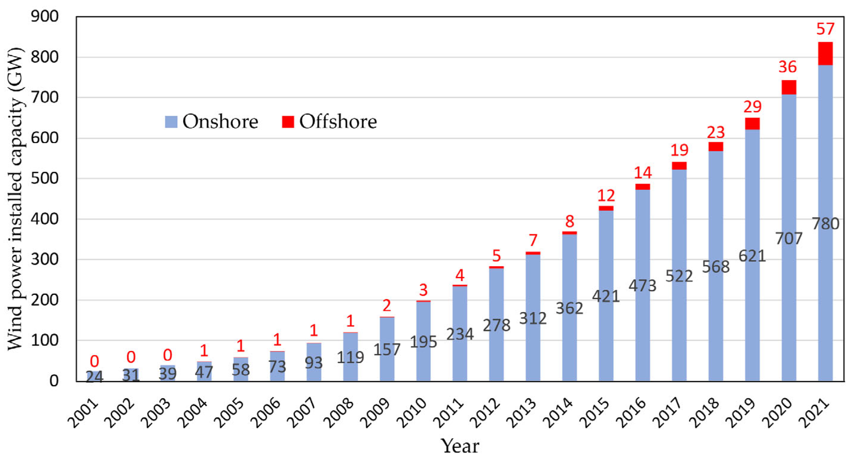
In recent decades, various renewable energies, such as wind, solar, waves, etc., have received increasing attention. Among all these energies, wind power has played the most important role in replacing fossil fuels [2]. As reported by the World Wind Energy Council, the installed global capacity of wind energy in the world in 2021 has reached 837 GW, with an increase of 92 GW compared to 2020 [3]. Figure 1 shows the global wind power installed capacity increment over the past 21 years [3]. In this figure, the blue columns represent the capacity of installed wind power on land, while the red columns represent the offshore installed wind energy.

One main obstacle hindering the increase of wind power penetration into the power grid is the production uncertainty due to fluctuations in wind speed [1]. Therefore, adequate planning in electricity distribution to meet consumers’ demand, determining the best time for operation and maintenance, and the fairest pricing on the market requires accurate wind power forecasting in the upcoming time steps.

Hanifi et al. [1] categorised wind power forecasting into three main methods, including physical, statistical, and hybrid approaches. Physical methods utilise numerical weather prediction (NWP) data, wind turbine geographic descriptions, and weather information to predict wind power [1]. These methods are computationally complex and very sensitive to initial information [2]. On the other hand, statistical methods work based on building an accurate mapping between input variables (such as NWP data, historical data, etc.) and target variables (wind speed or wind power). These methods include two main approaches: time-series-based methods and machine learning (ML) approaches [1]. Time-series-based methods can predict wind speed or wind power based on the history of the predicted variable itself. They can recognise the concealed random features of wind speed and are used for very short-term (minutes to a few hours) forecasting. The Auto-Regressive Integrated Moving Average (ARIMA) model proposed by Box–Jenkins [4] is one of the common statistical methods which is used in various research. For example, in Western Australia, Yatiyana et al. [5] applied the ARIMA model for wind speed and direction forecasting. They proved that their proposed model could predict wind speed and direction with a maximum of 5% and 16% error, respectively. Firat et al. [6] proposed an autoregressive (AR) wind speed prediction model for a wind farm in the Netherlands. They used six years of hourly wind speed and achieved a high accuracy for 2–14 h ahead. In another study, De Felice et al. [7] applied 14 months of temperature readings in Italy to train an ARIMA model for electricity demand prediction. Their proposed method demonstrated higher accuracy, particularly in hot locations, compared with persistence methods. Duran et al. [8] proposed a method to combine AR and exogenous variable (ARX) models to predict the wind power generation in a wind farm located in Spain up to one day in advance. They used different model orders and training periods to prove that the application of the AR models presents lower errors than a persistent model. Kavasseri et al. [9] examined the application of fractional ARIMA models to predict wind farm hourly average wind speed for one- and two-day-ahead time horizons. The results of the predictions showed a 42% improvement compared to persistent methods. Later, the predicted wind speeds were applied to the power curve of an operating wind turbine to predict the relevant wind powers. In another study, Torres et al. [10] used the ARMA and the persistence model for hourly average wind speed forecasting up to 10 h ahead. The ARMA model demonstrated a better performance compared to the persistence method, with a 12% to 20% lower root mean square error (RMSE) when forecasting 10 h in advance.

ML methods such as neural networks (NNs) can establish deductive models by learning dependencies between input and output variables. These methods are easy to create, do not require further geographic information, and can predict over longer timeframes. One of the common ML methods is the LSTM model, which can address the long-term dependency issues [11], which is important in forecasting time-series with long input sequences [12].

LSTM is variously used in research for wind power prediction. For instance, Zhang et al. [13] proposed an LSTM wind power forecasting model for three wind turbines of a wind farm in China. They utilised three months of wind speed and historical power data and achieved the highest forecasting accuracy in a one-to-five time-steps ahead compared to the radial basis function (RBF) and deep belief network (DBN). Fu et al. [14] demonstrated LSTM and gated recurrent unit (GRU) for a one-to-four step-ahead forecasting of a 3 MW wind turbine in China, based on the first three-month dataset of 2014, with a resolution of 15 min. The comparison with ARIMA and support vector machine (SVM) methods showed the superiority of their proposed methods. Cali and Sharma [15] proposed an LSTM-based model with one hidden layer for 1 to 24 h ahead of wind power forecasting. The model was trained with 9-month data and evaluated in the last three months of 2016. They used nine combinations of input data, including wind speed at various levels, wind direction, temperature, and surface pressure. They demonstrated that temperature, wind speed, and direction positively impacted model performance; however, adding surface pressure to the input features led to worse performance.

As well as the training data, ML models’ accuracy strongly depends on the adequate selection of their parameters and hyperparameters. The parameters of ML models (e.g., the weights of each neuron) are determined during the training process of the algorithm. In contrast, hyperparameters are not directly learnt by the learning algorithm and need to be specified outside the training process. The main role of the hyperparameters is to control the capacity of the models in learning dependencies. They also prevent overfitting and improve the generalisation of the algorithm. Hyperparameter optimisation or tuning improves forecasting accuracy and reduces models’ complexity [16].

The literature’s most common hyperparameter tuning methods are the grid search and random search. Grid search can be used for simple models with a few parameters. The calculation will be extremely time-consuming by increasing the number of parameters and expanding the space of the possible configurations [17]. Therefore, researchers usually consider a narrow range of hyperparameters during the grid search [16]. On the other hand, a random search algorithm looks randomly for a set of combinations rather than searching for better results.

Both these search methods generate all candidate combinations of hyperparameters upfront and then evaluate them in parallel. Based on the evaluation of all combinations, the best hyperparameters can be selected. Trying all possible combinations is very costly; as a result, it is vital to develop advanced techniques to intelligently select which hyperparameters to assess and then decide where to sample next after evaluating their quality.

The advanced optimisation of the ML-based time-series forecasting models for wind turbine-related predictions remained untouched. However, a few studies have proposed methods for optimising ARIMA and LSTM models within other applications than wind power forecasting. For example, Al-Douri et al. [18] designed a genetic algorithm (GA) to find the best parameters of an ARIMA model for the better cost prediction of used fans in Swedish road tunnels, and provided results which proved a significant improvement in data forecasting. In another study, F. Shahid et al. [19] employed GA to optimise the window size and neuron numbers of LSTM layers. This approach improved the power prediction accuracy of wind farms in Europe by up to about 30% compared to existing methods such as support vector regressors.

As the review of the literature indicates, several examples use linear and nonlinear regression models for challenges related to predicting wind power. Each study provides the use of one model type or a comparison of various model types. Nevertheless, without the tuning and selection of the hyperparameters, it is not possible to obtain their maximum benefit [16]. This advanced tuning method plays an important role when the hyperparameter search space grows exponentially, and the use of exhaustive grid search becomes extremely time-consuming.

This paper proposes a framework for developing accurate and robust ML models for wind power forecasting. The framework outlines the model development procedure from data engineering to precision evaluation and fine-tuning. Furthermore, an advanced algorithm is utilised to optimise wind power forecasting models to reduce time calculation costs, as well as to improve accuracy. For the case study, two ML models were selected: the LSTM model, which is proven to have remarkable prediction performance on time-series-based models, and ARIMA, a traditional model, for the purpose of benchmarking.

The novelty of this work lies in developing a short-term wind power forecasting model through an intelligent application of the long short-term memory (LSTM) model, while a new optimisation algorithm tunes its main hyperparameters. In addition, the distinguished aspects of the methodology are summarised, based on importance, as follows:

• LSTM is used on a wind power dataset to take advantage of its ability to learn nonstatic features from nonlinear sequential data automatically.
• The ARIMA model is applied as a forecasting model because of its short response time and ability to capture the correlations in time series.
• Instead of the trial-and-error method to select the best hyperparameters of the ARIMA and LSTM forecasting models, which require a great deal of time, grid search is used to tune both these models.
• The new Optuna optimisation framework is employed to optimise the hyperparameters of the LSTM model, including the number of lag observations, the quantity of LSTM units for the hidden layer, the exposure frequency, the number of samples inside an epoch, and the used difference order for making a nonstationary dataset stationary.
• Unlike most previous studies, which is for onshore wind turbines, forecasting assessments have been done for an offshore wind turbine in this study.
• How to deal with the negative values of wind power (which are normally found in active power observations), in terms of removal or replacement, has been thoroughly investigated in this study and the results have been discussed.
• After a detailed discussion about the reasons for having outliers, three different methods, including isolation forest (IF), elliptic envelope (EE), and the one-class support vector machine (OCSVM), are used to detect and treat them. A comparison of the results will help researchers to choose the best outlier detection method for future studies.
• The proposed Optuna–LSTM model is assessed by the comparison of its forecasted power with actual values and predictions by persistence and ARIMA based on the RMSE statistical error measure.

The rest of this paper is organised as follows: Section 2 discusses the optimisation process, the forecasting models, and the studied supervisory control and data acquisition (SCADA) data. This section includes the steps taken for preprocessing, resampling, and outlier treatment. Section 3 presents the results of the trained, optimised LSTM model in terms of model accuracy and the time cost compared to other prediction methods. Finally, Section 4 summarises the paper’s contributions.

2. Methodology

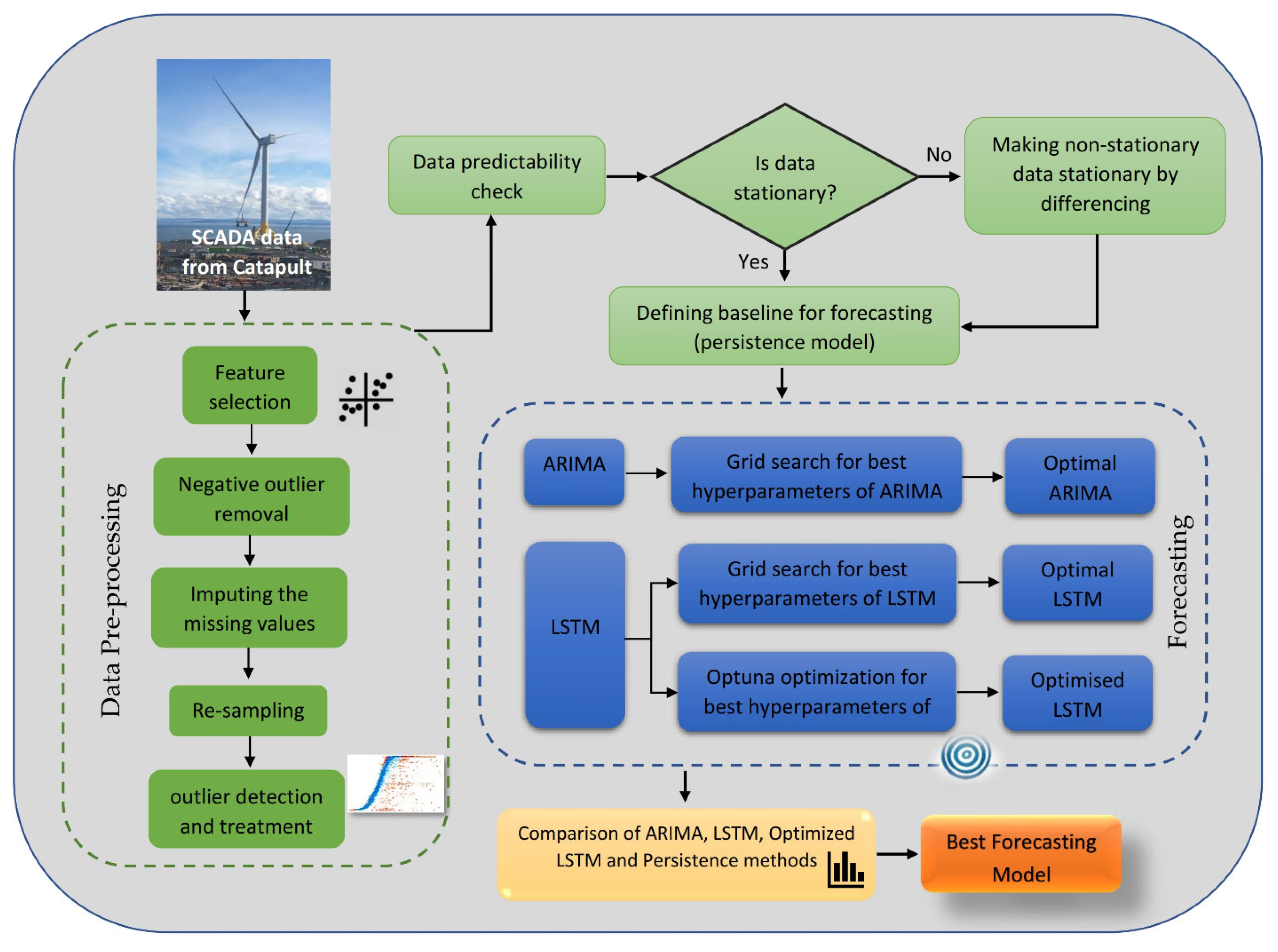
The proposed procedure of this study is illustrated in Figure 2. At the beginning of this study, three required features, including the time stamps, wind speeds, and active wind powers, are selected to improve the computational time. At the next step, negative power values are removed or replaced. This data preprocessing is followed by resampling the dataset and removing outliers in three different ways. After finishing the data preprocessing and providing proper data for forecasting, data predictability and stationarity are assessed as two important specifications for accurate power forecasting. Afterwards, three different approaches are employed for forecasting, and their best performance is gained by the selection of their most appropriate hyperparameters.

2.1. ARIMA Model

In this study, the standard approach of the Box–Jenkins method [20] was traced for the ARIMA model development. The ARIMA model is a widely used set of statistical models for analysing and predicting time-series data [21]. This model can be expressed as [22]:

$$X_t={\varphi }_1{X}_{t-1}+{\varphi }_2{X}_{t-2}+\cdots +{\varphi }_p{X}_{t-p}+e_t-{\theta }_1{e}_{t-1}-{\theta }_2{e}_{t-2}-\cdots -{\theta }_q{e}_{t-q}$$

(1)

While ${\varphi }_t$ and ${\theta }_t$ are coefficients, p, q, and d are the lag number of observations in the model, the order of moving average, and the degree of difference, respectively. Degree of difference (d) values greater than 0 imply that the data has been nonstationary but has become stationary after some degree of difference.

The ARIMA model combines the AR, moving average (MA), and the Integrated (I) components, which denotes the data substitution with the value of the difference between its values and the preceding values [23]. The forecasting accuracy of the ARIMA model depends on selecting the most appropriate combination of p, d, and q. Normally, for small data sets, the autocorrelation function (ACF) and partial autocorrelation function (PACF) can be used to determine which AR or MA component should be selected in the ARIMA model [24].

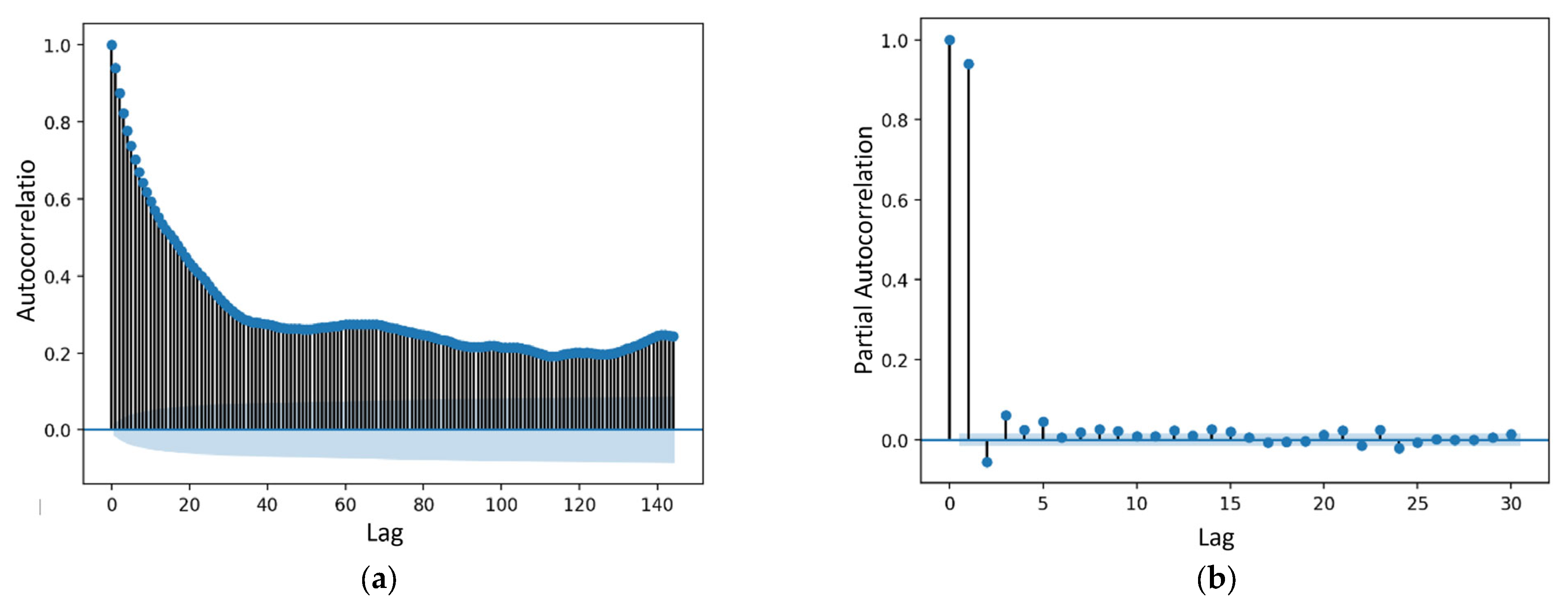
These two factors, which can be graphically plotted, are widely used elements in analysing and predicting time-series. They highlight the relationship between an observation and the observations’ value at prior time steps. The difference between ACF and PACF is that, in PACF, while assessing the relationship between observation of two time steps, the relationships of the intervening observations are removed. Figure 3a,b show the observations’ ACF and PACF plots. An appropriate ARIMA model can be selected based on the simple explanations in

Table 1. ACF and PACF application for statistical model selection.

Model	Autocorrelation	Partial Autocorrelation
AR (p)	Tails off gradually	Cuts off after p lags
MA(q)	Cuts off after q lags	Tails off gradually
ARMA (p, q)	Tails off gradually	Tails off gradually

[9], and the value of d (degree of difference) depends on the number of differencing until the data is stationary.

The ARIMA model forecasting steps after resampling and outlier treatment can be seen in Figure 4. The first step is assessing the stationarity of the time-series. Stationary is one of the assumptions during time-series modelling, which shows the consistency of the summary statistics of the observations.

When a time-series is stationary, it means that the statistical properties of the time-series (such as mean, variance, and autocorrelation) do not change over time. This property can be violated by having any trend, seasonality, and other time-dependent structures. There are two main methods for the stationarity assessment of time-series, the visualisation approach and the augmented Dickey–Fuller (ADF) test. The visualisation method uses graphs to show whether the standard deviation changes over time. On the other hand, the ADF method is a statistical significance test that compares the p-value with the critical values and does hypothesis testing. This test makes the stationarity of data clear at different levels of confidence.

Regarding the data used in this study, due to the high number of observations and wide dispersion, it is not possible to check stationarity through the visualisation method. Therefore, in this study, the ADF method was used.

The ADF test’s execution provides a p-value which, by comparing it with a threshold (such as 5% or 1%), can identify the stationarity of the data. Nonstationary data in this step need to be changed to stationary by methods such as differencing. After ensuring the time-series is stationary, a persistence method as a baseline is created. Then, through a detailed grid search, the best hyperparameters for the ARIMA forecasting for each preprocessed data were found. The last step is ARIMA forecasting and comparing its error with the error of the persistence method.

2.2. LSTM Model

The recurrent neural network (RNN) is a model in which the connection of its units creates cycles. RNN has a high ability to represent all dynamics. However, its effectiveness is affected by the limitations of the learning process. The main limitation of gradient-based methods that use back propagation is their path integral time-dependence on assigned weight [13]. When the time lag between the input signal and the target signal increases to more than 5–10 time-steps, the normal RNN loses the learning ability, and the back-propagation error either vanishes or explodes. This error elimination raises the question of whether normal RNNs can show practical benefits for feed-forward networks. To address this problem, the LSTM has been developed based on memory cells. The LSTM consists of a recurrently attached linear unit known as the constant error carousel (CEC). CECs, by keeping the local error backflow constant, mitigate the gradient’s vanishing problem [25]. They can be trained by adjusting both the back propagation over time and the real-time recurrent learning algorithm [26]. 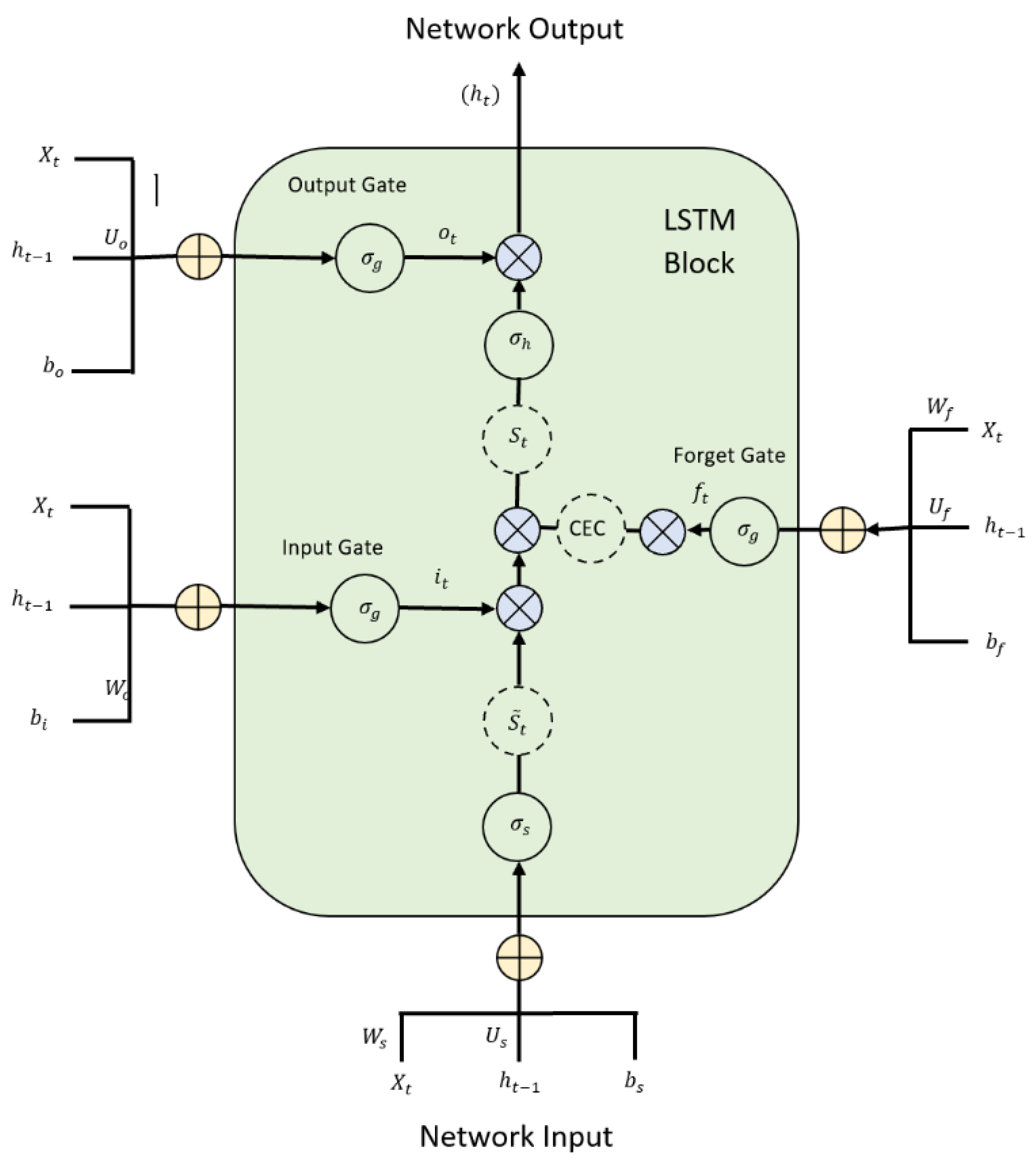Figure 5 shows the typical structure of the LSTM.

As can be seen, there are three gate units in a basic LSTM cell, including the input, output, and forget gates. The gate activation vectors of $i_t$, $o_t$ and $f_t$ for input, output, and forget gates, respectively, are calculated in Equations (2)–(4).

$$i_t={\sigma }_l\left(W_i{x}_t+U_i{h}_{t-1}+b_i\right)$$

(2)

$$o_t={\sigma }_l\left(W_o{x}_t+U_o{h}_{t-1}+b_o\right)$$

(3)

$$f_t={\sigma }_l\left(W_f{x}_t+U_f{h}_{t-1}+b_f\right)$$

(4)

In these equations, $W_i$, $W_o$, $W_f$ $U_i$, $U_o$, and $U_f$ represent the assigned weights, and $b_i$, $b_o$, and $b_f$ represent the biases in conjunction with relevant activation functions ${\sigma }_l$. In addition, $x_t$ is the neuron input at time step t, and the cell state vector at time step t − 1 is $h_{t-1}$. As shown in Equation (5), the next evaluated value of the state ${\tilde{S}}_t$ can be calculated based on the relevant activation function ${\sigma }_s$.

$${\tilde{S}}_t={\sigma }_s\left(W_s{x}_t+U_s{h}_{t-1}+b_s\right)$$

(5)

In Equation (7), the newly assessed value of ${\tilde{S}}_t$ and the prior cell state $S_{t-1}$ are used to calculate cell state $S_t$, which by itself will be used with the output gate control signal $o_t$ and the activation function ${\sigma }_{lh}$ to obtain the overall output $h_t$ according to Equation (8).

$$S_t=f_t◦S_{t-1}+i_t◦{\tilde{S}}_t$$

(6)

$$h_t=o_t◦{\sigma }_{lh}\left(S_t\right)$$

(7)

As can be seen in Equations (6) and (7), the output $h_t$ is dependent on the state $S_t$ of the LSTM cell and the activation function ${\sigma }_{lh}$ that is usually tanh (x). The state $S_t$ depends on the state of the prior step $S_{t-1}$ as well as the new value of the state ${\tilde{S}}_t$.

In accordance with all the relations mentioned above, the function of the LSTM model can be concluded as:

• Input gate ($i_t$) controls the extent to which ${\tilde{S}}_t$ flows into the memory.
• Output gate ($o_t$) regulates the extent to which $S_t$ gives to the output (ht).
• Forget gate ($f_t$) controls the extent to which $S_{t-1}$ (i.e., previous state) is kept in the memory.

Specifying the best LSTM model for wind power forecasting requires the determination of the neural network’s best combination of hyperparameters. LSTMs have five main hyperparameters, including the number of lag observations as inputs of the model, the quantity of LSTM units for the hidden layer, the model exposure frequency to the whole training dataset, the number of samples inside an epoch in each weight updating, and finally, the used difference order for making nonstationary data stationary.

2.3. Grid Search for ARIMA and LSTM Models

ARIMA model factors (i.e., p, d, and q) can be estimated through iterative trial and error by revising the ACF and PACF plot. This part of defining the ARIMA forecasting model can be very challenging and time-consuming, leading to prediction errors. As a result, researchers attempt to find these hyperparameters using an automatic grid search approach. Similar to the ARIMA model, specifying the best LSTM model for wind power forecasting requires the determination of the best combination of hyperparameters in this neural network. This study also specified a grid of the LSTM parameters to iterate. An LSTM model is created based on each combination, and its forecasting accuracy is assessed by calculating its RMSE.

2.4. Persistence Method

It is vital to create a baseline for any time-series prediction approach. As a reference, for comparing all modelling approaches, this baseline can show how well a model makes predictions. Models which perform worse than the performance level of the baseline can be ignored.

Benchmarks for forecasting problems need to be very simple to train, fast to implement, and repeatable. The persistence model is one of the most commonly used references for wind speed and power prediction (short-term forecasting methods in particular). Based on the definition of this method, wind power in the future will be equivalent to the generated power in the present [27], as given by Equation (8):

$${\widehat{P}}_{t+k/t}=P_t$$

(8)

where $P_t$ is the measured wind power at time t and ${\widehat{P}}_{t+k/t }$ is the predicted wind power for the future time k. This model performs better than most short-term physical and statistical forecasting methods. Therefore, it is still widely used in very short-term prediction [28]. This research uses the persistence model to compare the performance of the ARIMA and LSTM models for different datasets.

2.5. Hyperparameter Optimisation with Optuna

This study uses the Optuna optimisation method to optimise the forecasting models. Optuna is an open-source optimisation software with several advantages over the other optimisation frameworks [29]. Other optimisation tools usually differ depending on the algorithm used to select the parameters. For example, GPyOpt and Spearmint [30] apply Gaussian processes, SMAC [31] employs random forests, and Hyperopt [32] uses a tree-structured Parzen estimator (TPE). These methods have three main drawbacks. Firstly, they need the parameter search space to be statically defined by the user, a process that is extremely hard for large-scale experiments with many possible parameters. Furthermore, they do not have an efficient pruning strategy for high-performance optimisation when accessing limited resources. In addition, they cannot handle large-scale experiments with minimal setup requirements. On the other hand, Optuna, with a define-by-run design, enables the user to create the search space dynamically. This optimisation framework is an open-source, easy-to-set-up package that benefits effective sampling and pruning algorithms [29]. Optuna optimises the model through minimising/maximising an objective function (here, the RMSE of the forecasted wind power rather than the real generated values) that assumes a group of hyperparameters as input and returns its validation core. The optimisation process is called a study, and each objective function’s evaluation is called a trial [29].

At the beginning of the optimisation, the user is asked to provide the search space for the dynamic generation of the hyperparameters for each trial. Then, the model builds the objective function by interacting with the trial object. After this step, the next hyperparameter selection is based on the history of previously evaluated trials. This algorithm optimises ML models in two steps. First, a search strategy determines a set of parameters to be examined, and second, a performance assessment strategy known as a pruning algorithm excludes the improper parameters based on the estimation of the value of the currently investigated parameters [29].

Since the initial prediction accuracy assessment of the ARIMA and LSTM models (both tuned by grid search) highlighted the better performance of the LSTM model compared to ARIMA, it was decided to apply the optimisation framework only to the LSTM model.

In this way, the hyperparameter ranges of the LSTM model increased from what was examined in its grid search to wider ranges, as shown in

Table 2. Hyperparameter ranges and their total combinations in LSTM–grid search and LSTM–Optuna methods.

Parameters	LSTM–Grid Search		LSTM–Optuna
	Values	Possible Combinations	Values	Possible Combinations
No. of lag observations	(3, 4, 6)	48	(1, 3, 4, …, 10)	More than 1 M
No. of LSTM units	(100, 150)		(50, 60, 70, …, 300)
Exposure frequency	(100, 150)		(50, 60, 70, …, 300)
No. of samples inside an epoch	(100, 150)		(50, 60, 70, …, 300)
Difference order	(0, 1)		(0, 1, 2, …, 5)

. In other words, the hyperparameter combinations increased from 48 combinations to more than a million combinations.

2.6. Wind Power Dataset

The source SCADA data are measured at a 1 Hz frequency from the Levenmouth Demonstration Turbine (LDT), an offshore wind turbine which is located just 50 m from the coast at Leven, a seaside town in Fife, Scotland [33]. This wind turbine was acquired by the Offshore Renewable Energy (ORE) Catapult in 2015, while its construction was completed by Samsung in October 2013 [34].

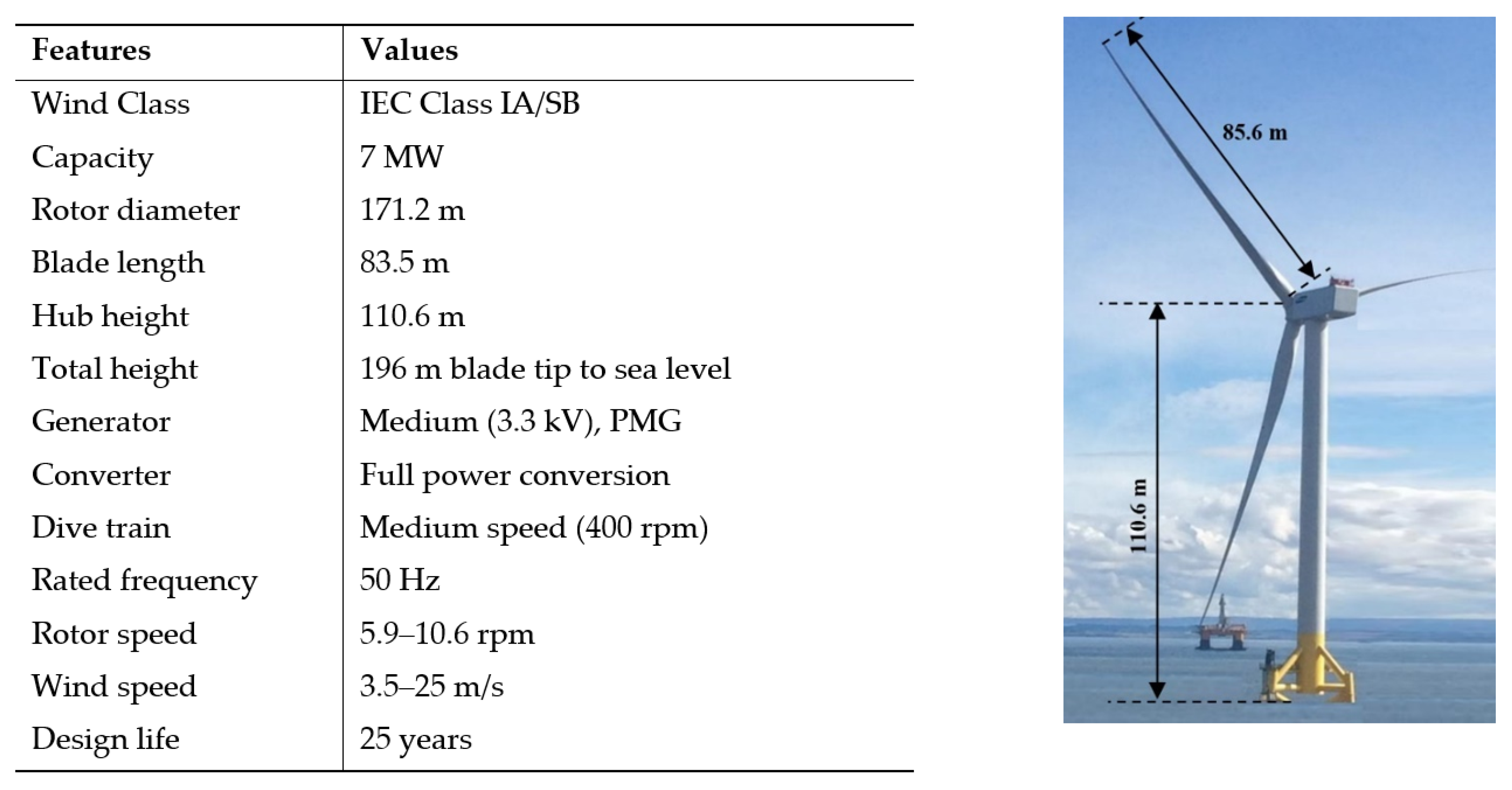
ORE Catapult’s wind turbine is a three-bladed upwind turbine installed on a jacket structure [25]. The turbine is ranked to work at 7 MW, but to decrease the noise, it is limited to operating at the highest power of 6.5 MW [33]. This turbine’s rotor diameter is 171.2 m, and its hub height is 110.6 m. Each blade of this turbine measures 83.5 m and weighs 30 tons. The defined cut-in speed for this turbine is 3.5 m/s, which means its electricity generation will start when wind speeds reach this speed. It will shut down if the wind is blowing too hard (roughly 25 m/s) so to prevent equipment damage. Its operating temperature is between −10 °C to +25 °C, and it has been designed to work for 25 years [35]. Figure 6 shows the configuration and main parameters of the LDT.

2.7. Feature Selection

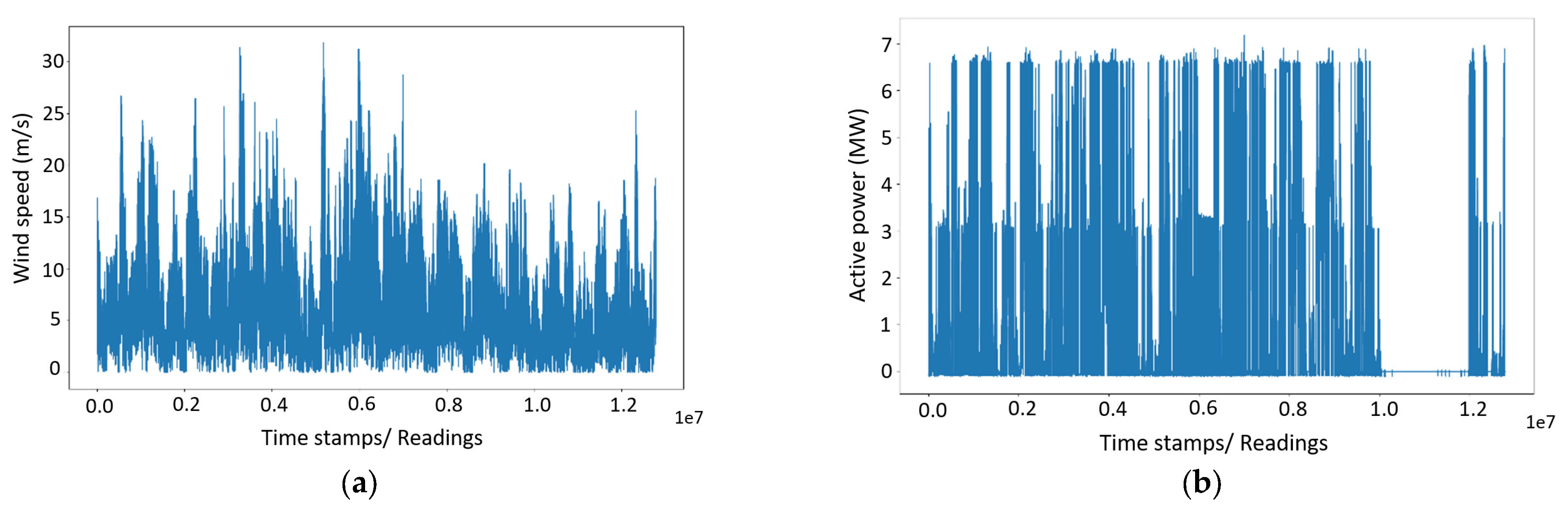
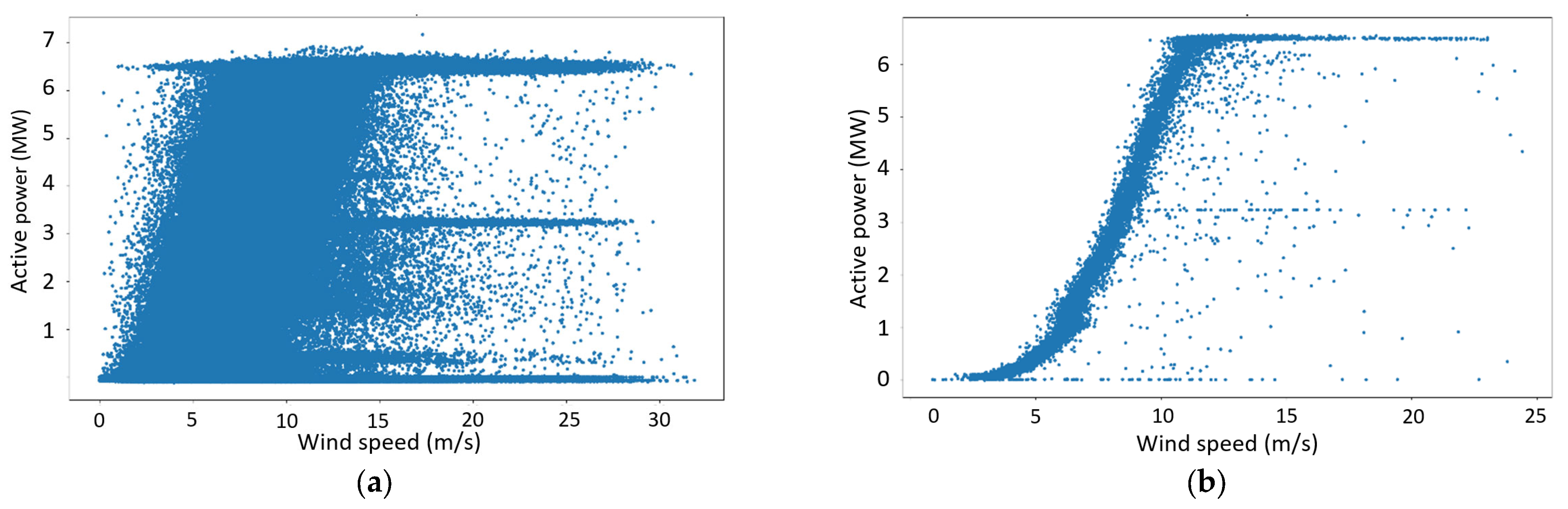
This study recorded the SCADA datasets for five months, from 1 January 2019 to 31 May 2019, at a 1 Hz frequency (with one-second intervals). Each timestamp in this time-series data includes 574 different observations, including the generated power, wind speed at different levels, blade pitch angle, nacelle orientation, etc. At the beginning of the data processing, a feature selection was carried out to decrease the size of the dataset to reduce the computation time by excluding unnecessary variables. This process was vital to making this study possible. All variables except the time stamp, wind speed, and active power were removed at this stage, which was useless in the ARIMA and univariate LSTM forecasting methods. Keeping the wind speed variable was vital in this project, as it verified the accuracy of generated power. For example, failure to generate power when high wind speeds were recorded was recognised as a stop in power generation due to reasons such as maintenance. After removing the redundant information, observations of wind speed and active power were plotted as shown in Figure 7a,b.

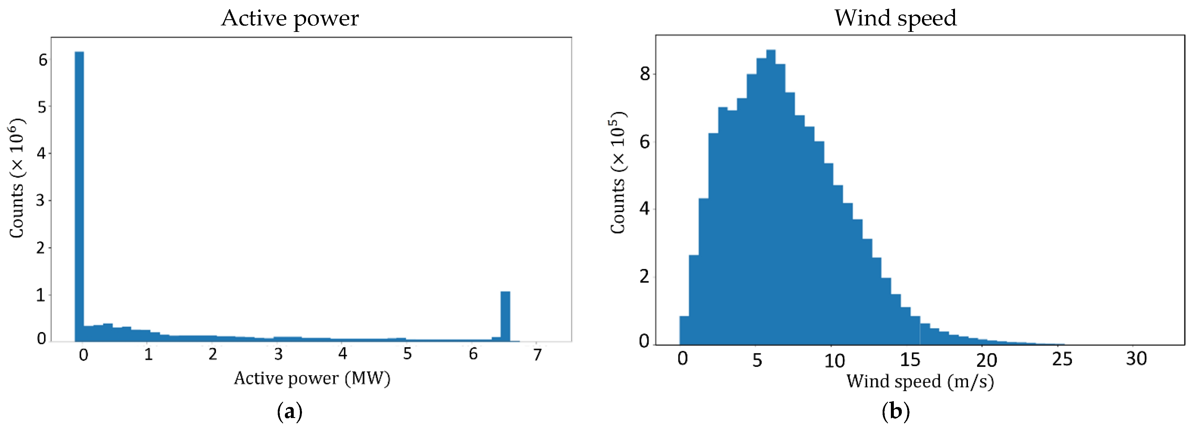
The histograms of this dataset for wind speed and active power are presented in Figure 8a,b, and

Table 3. Statistical descriptions of the SCADA datasets.

	Active Power, kW	Wind Speed, m/s
Count	$1.0\times {10}^7$	$1.0\times {10}^7$
Mean	$1.8\times {10}^3$	7.6
Standard deviation	$2.3\times {10}^3$	3.9
Minimum	$-1.2\times {10}^2$	$-3.3\times {10}^{-2}$
25%	$-6.0\times 10$	4.7
Medium	$5.9\times {10}^2$	7.1
75%	$3.2\times {10}^3$	$1.0\times 10$
Maximum	$7.2\times {10}^3$	$3.2\times 10$

shows their statistical descriptions.

2.8. Obvious Outlier Removal

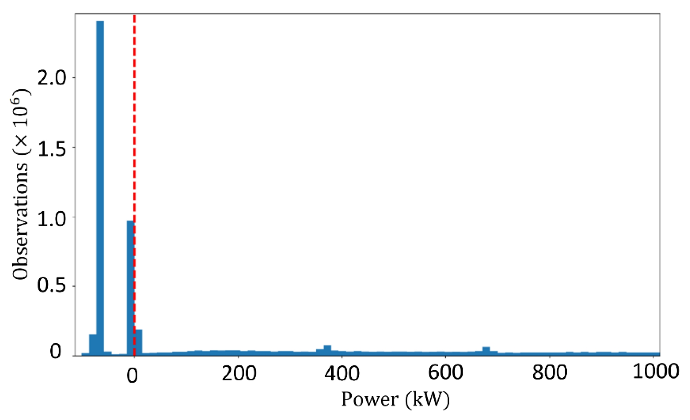
An initial assessment of Figure 7b specified that a large part of the recorded generated power at the end of this time-series (May 2019) equals zero. Usually, the generated power of a turbine can be zero when no wind is blown. However, the evaluation of Figure 7a shows a continuous wind blowing with fluctuations similar to previous months. Therefore, it is speculated that the turbine was out of production during this period. Based on this assumption, it was decided that this month (May 2019) should be removed entirely from the dataset. The time-series after this omission was reduced to four months, from 1 January 2019 to 30 April 2019. A closer look at the active power, as shown in Figure 9, revealed another obvious error in the SCADA data, the existence of negative values. Negative values are values of which there is no practical meaning in wind power generation. Shen et al. [36] believe that these values represent time stamps when turbine blades do not rotate, but the turbine’s control system needs electricity [36]. These values need to be eliminated along with the corresponding parameters of the same timestamp for better forecasting results [25]. Since the elimination of these negative values disrupts the time continuity of the time-series, and can possibly lead to errors in wind power prediction, at this stage it was decided to create and assess three types of datasets based on different actions against negative values. Assessment of the impact of these actions on forecasting accuracy became another goal of this study.

These three preprocessing methods against the negative values are:

• Total elimination of negative values without any substitution;
• Replacement of negative values with the average amount of power in the whole 4-month period;
• Replacement of negative values with positive values of power at the nearest timestamp.

2.9. Resampling

The effect of wind turbulence as one of the obstacles to increasing the wind energy penetration in energy markets is more significant in horizontal axis wind turbines. This is because the wind speed and direction change rapidly after hitting swept blade rotors. Therefore, the amount of wind speed measurements by installed anemometers are not equal to the speed of the wind flow hitting turbine blades [25]. These differences, which lead to a decrease in the correlation between the measured wind speed and the output power, and then scattering of the power curve, can be resolved by averaging the samples in a reasonable average period [25]. The SCADA data for this study was recorded with a 1 Hz frequency; as a result, it was possible to create multiple averaged sets for removing the mentioned obstacle. According to a review conducted by Hanifi et al. [1], the maximum sampling rate used for wind speed and power forecasting in the previous research is 10 min. This is equivalent to an average time that the international standard for power performance measurements of electricity-producing wind turbines (IEC 61400-12-1) establishes for large wind turbines [37]. Based on the IEC 61400-12-1 and reviewed literature, the data presented here was averaged for each 10 min of data collection. 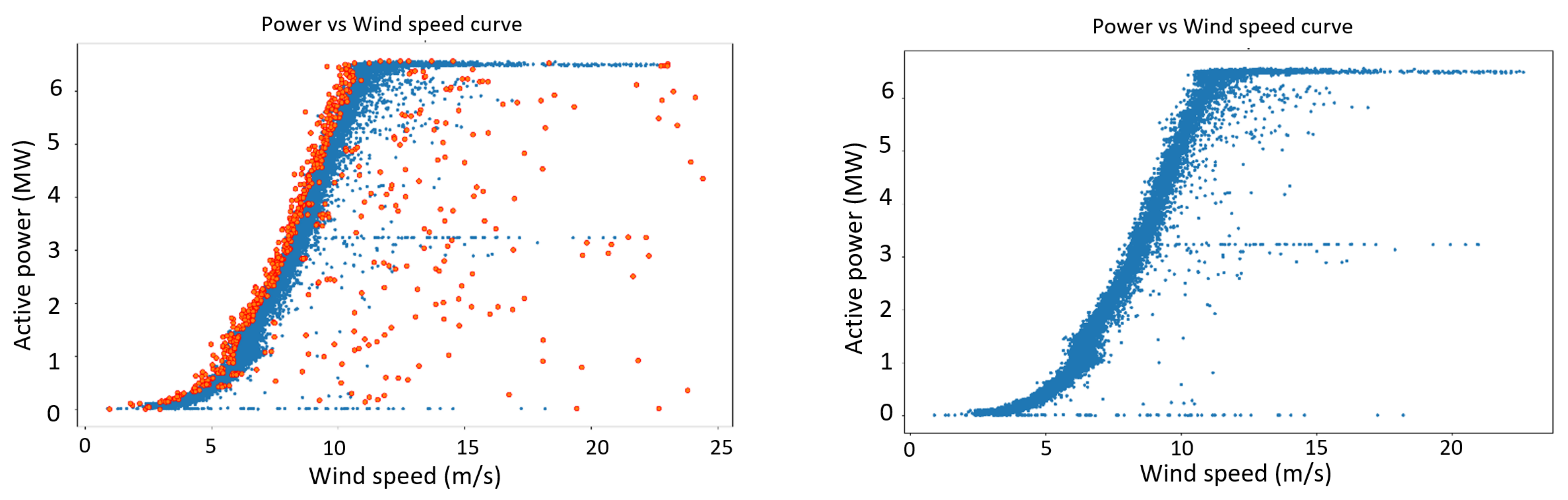Figure 10a,b show the wind power curves for the original and 10 min resampled data.

2.10. Anomalies Detection and Treatment

Outliers in a dataset are specific data points that are different or far from most other regular data points [38]. Undetected or improperly treated anomalies can adversely affect wind power forecasting applications. They may be biased with high prediction errors [38].

There are various reasons for having outliers among wind turbine and wind farm measurements, including wind turbine downtime [36], data transmission, processing or management failure [39], data acquisition failure [40], electromagnetic disturbance [36], wind turbine control system fault (such as the pitch control system fault) [41], damage of the blades or the existence of ice or dust [42], shading effect of neighbouring turbines, fluctuation of air density [43], etc.

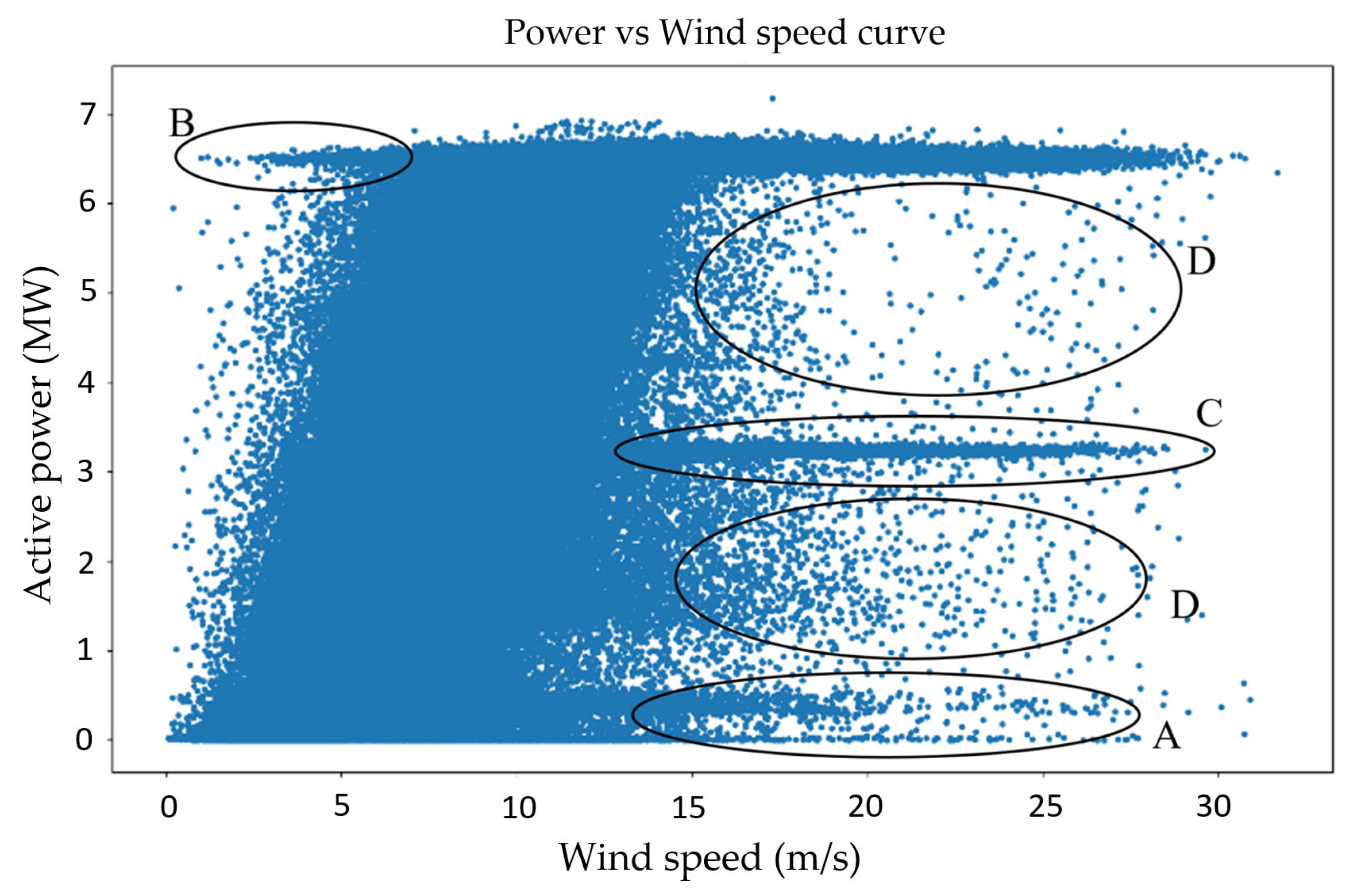
Figure 11 shows four different types of anomalies in the current SCADA data. Category A points have negative, zero, or low values of generated power during speeds larger than the cut-in speed [25]. The leading causes of these outliers are wrong wind power measurements, wind turbine failure, and unexpected maintenance. Wind speed sensors and communication errors cause category B outliers. The mid-curve outliers (category C) represent power values lower than ideal—this is caused by the down-rating of the wind turbines and data acquisition. Outliers in category D are scattered irregular points due to faulty sensors exacerbated during harsh weather circumstances [36].

There are different methods for anomaly detection in machine learning, such as Density-Based Spatial Clustering of Applications with Noise (DBSCAN), IF, local outlier factor, and EE. In this study, three common methods for wind power forecasting are investigated. EE is used based on the assumptions described in [44]. IF, which is an unsupervised learning algorithm, recognises anomalies by isolating them in the data. This algorithm works based on two main features of anomalies, that they are few and different. The one-class support vector machine (OCSVM) is a common unsupervised learning algorithm for outlier detection, assuming rare anomalies create a boundary for most data, and considering data points out of the boundary as outliers [45]. This method of outlier detection and treatment chose the third method.

3. Experimental Results and Discussion

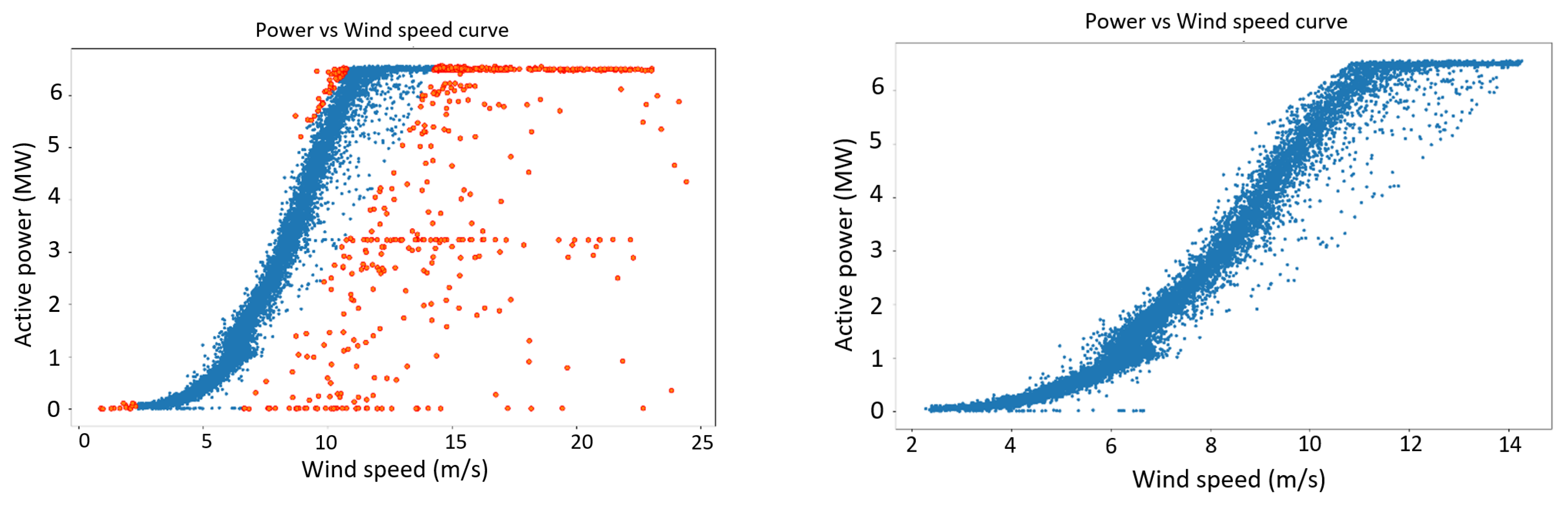
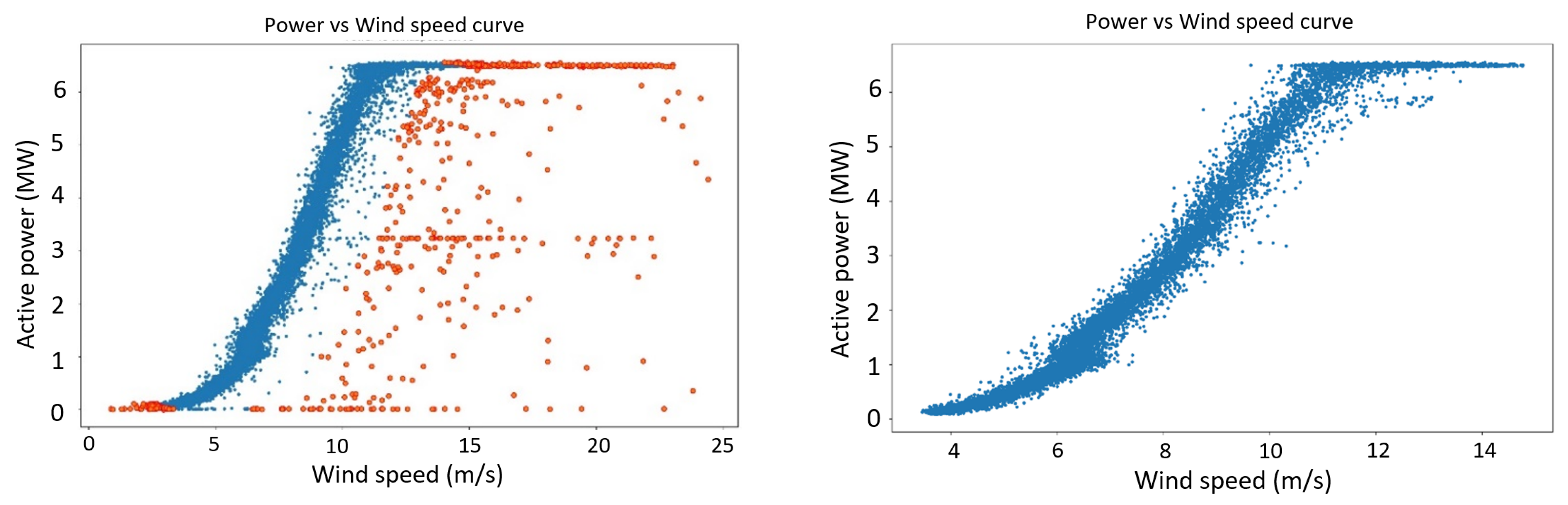
This research employs packages and subroutines written in Python to implement the proposed algorithms. A PC with an Intel Core i5–7300 32.6 GHz CPU and 8 GB RAM (without any GPU processing) was used to run the experiments. Three outlier detection methods, which were described in Section 2.8, were used to detect and remove the outliers of the resampled dataset. The results of these treatments can be seen in Figure 12, Figure 13 and Figure 14:

This study considers six different preprocessing methods based on applying three different outlier detection methods and three approaches against the negative power values (

Table 4. Best ARIMA and LSTM hyperparameters resulting from the grid search.

Case Data	Preprocessing Approach	ARIMA Hyperparameters	LSTM Hyperparameters
Case 1	Negatives replaced by mean *; Outliers not removed	(2, 0, 1)	(3, 100, 100, 150, 0)
Case 2	Negatives replaced by nearest positive value *; Outliers not removed	(1, 1, 1)	(6, 100, 150, 150, 0)
Case 3	Negatives removed; Outliers not removed	(1, 0, 2)	(3, 100, 150, 150, 0)
Case 4	Negatives removed; Outliers removed by EE method	(1, 1, 3)	(3, 100, 100, 150, 0)
Case 5	Negatives removed; Outliers removed by IF method	(3, 1, 1)	(3, 150, 150, 150, 0)
Case 6	Negatives removed; Outliers removed by OCSVM method	(1, 1, 3)	(3, 150, 150, 150, 0)

*: Mean value has been calculated after removing negative values.

). Different cases of preprocessed data are fed to the ARIMA and LSTM forecasting models. The grid search method is applied for the initial hyperparameter tuning; Table 4 shows the selected hyperparameters for the ARIMA and LSTM models. As expected, the values of the hyperparameters vary depending on the different employed preprocessing methods (Table 4).

After selecting the best ARIMA and LSTM prediction methods, both models were trained by the first 95% part of the dataset (as training data) to make predictions for the last 5% of the dataset. The predicted values were compared with the measured values to determine the RMSE of each forecasting process.

Table 5. RMSE values of persistence, ARIMA, and LSTM models for six different treated case data.

	Data 1	Data 2	Data 3	Data 4	Data 5	Data 6
Negative values	Mean 1	Nearest Positive 2	Removed	Removed	Removed	Removed
Outliers	Not removed	Not removed	Not removed	EE removed	IF removed	OCSVM removed
Persistence	636.3	720.5	830.5	512.7	509	566
ARIMA	622.8	713	813	505.3	503.3	559
LSTM	626	695.8	785	501.5	497.5	550.6

¹ Replaced by mean value calculated after removing negative values. ² Replaced by nearest positive value.

provides the RMSE values of the ARIMA, LSTM, and persistence methods.

Comparing the RMSE values of all three models (Table 5) for case data 1, 2, and 3 clarifies that the complete elimination of the negative values (without any replacement) will lead to worse forecasting. The highest RMSE value of case 3 means that removing the negative values will decrease the forecasting accuracy. One of the reasons for this performance drop can be the creation of discontinuity in the dataset.

Regarding the best specific value to be considered instead of negatives, a comparison of case data 1 and 2 proves that replacing the negative values with the average wind power values has a better impact than replacing them with the nearest (neighbour) positive value. Replacing the negative values with the average values can lead to about a 15% forecasting improvement for ARIMA and 11% for the LSTM models.

The results also highlight the importance of dealing with outliers in wind power forecasting. Cases 4, 5, and 6, representing the outlier removed data, show a significant enhancement of the accuracy rather than the other cases, without any action against the anomalies. Comparing the error levels of case data 3 with cases 4, 5, and 6 (for both ARIMA and LSTM models) shows a 30% to 38% forecasting improvement by the elimination of the outliers, either by isolation forest, elliptic envelope, or the one-class SVM outlier detection methods.

The assessment of the RMSE values of cases 4, 5, and 6 show that the IF and EE outlier detection methods overcome the OCSVM method. An elliptic envelope can improve forecasting performance up to 9.61% and 8.92% rather than OCSVM for ARIMA and LSTM methods. This performance enhancement can reach 9.96% and 9.64% for ARIMA and LSTM, respectively, by applying the isolation forest.

As shown in Table 5, the ARIMA and LSTM methods for all the treated case data have better performances than the persistence methods. This is understandable if one remembers that, in the persistence method, only one preceding step data is used for forecasting, whilst the ARIMA and LSTM models consider a more extensive range of prior data.

It is also clear that the LSTM performs better than the ARIMA almost for all approaches against the negative values and outliers. This is probably due to the fact that LSTMs are better equipped to learn long-term correlation. In addition, the LSTM can better capture the nonlinear dependencies between the features.

In this study, because of the better prediction performance of the LSTM model compared to the ARIMA model, the proposed optimisation algorithm is applied to the LSTM model to tune its hyperparameters even more. As discussed in Section 2.5, the hyperparameter ranges of the LSTM model are increased from what was examined in its grid search to the wider ranges shown in Table 2.

The six preprocessed case data are again divided into the first 95% as the training dataset and the rest 5% as the test data. These divisions were developed to establish the same conditions and logically compare the new and previous methods. The developed optimisation algorithm, with the two described strategies, including search and pruning, started the selection of different combinations to minimise the RMSE value.

Table 6. Best LSTM hyperparameters resulted from Optuna optimisation.

Case Data	Preprocessing Approach	LSTM Hyperparameters
Case 1	Negatives replaced by mean *, Outliers not removed	(9, 190, 230, 130, 0)
Case 2	Negatives replaced by nearest positive value *, Outliers not removed	(8, 60, 270, 170, 0)
Case 3	Negatives removed; Outliers not removed	(3, 120, 120, 160, 0)
Case 4	Negatives removed; Outliers removed by EE method	(6, 180, 180, 180, 0)
Case 5	Negatives removed; Outliers removed by IF method	(4, 260, 120, 280, 0)
Case 6	Negatives removed; Outliers removed by OCSVM method	(2, 130, 280, 90, 1)

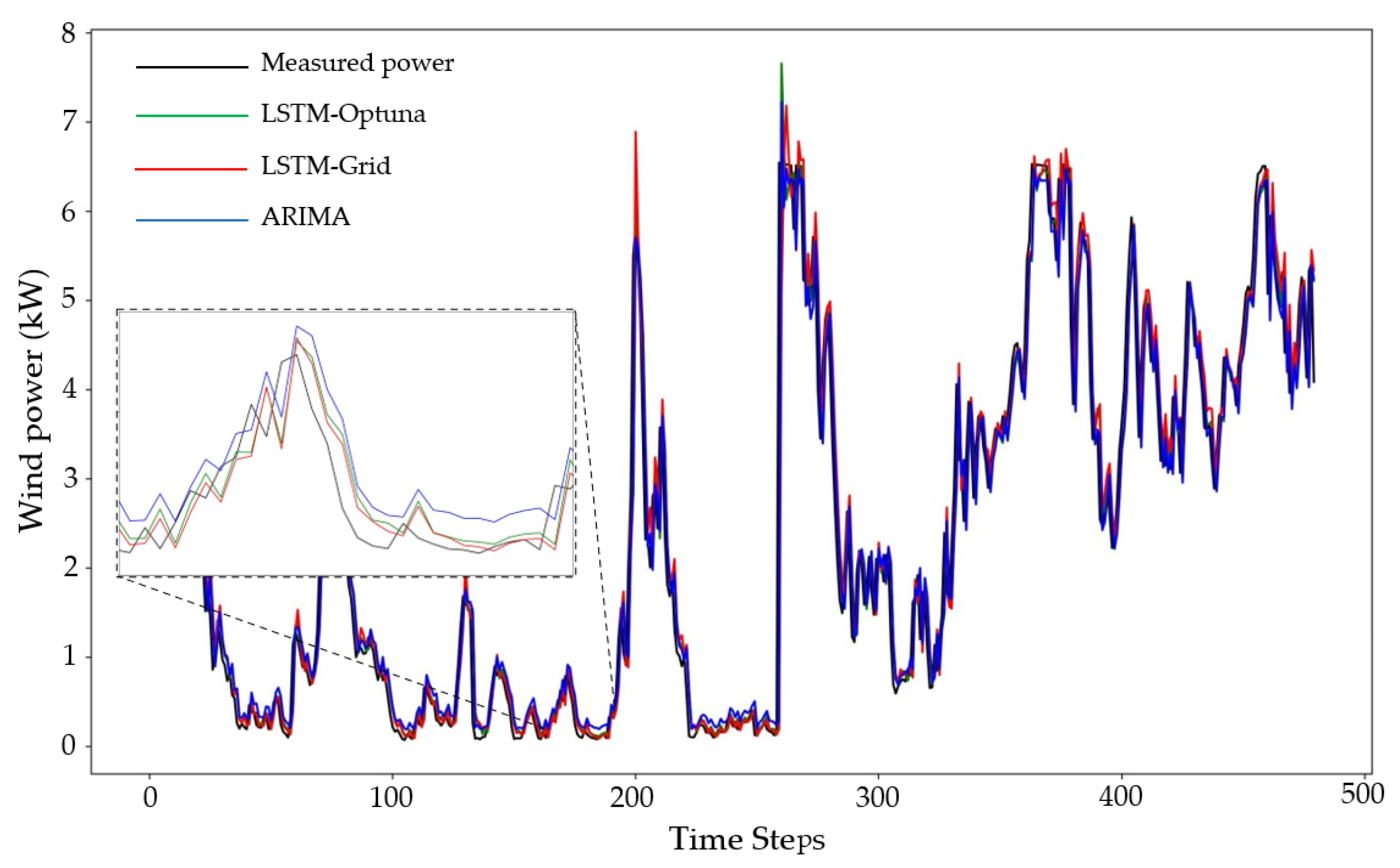
*: Mean value has been calculated after removing negative values.

shows the new hyperparameters found by the Optuna optimisation algorithm, and Figure 15 shows the measured power values of the turbine and prediction results of all the forecasting methods, including ARIMA, LSTM–grid, and LSTM–Optuna, for one of the datasets (data 4—removed negative values and removed outliers with the EE method).

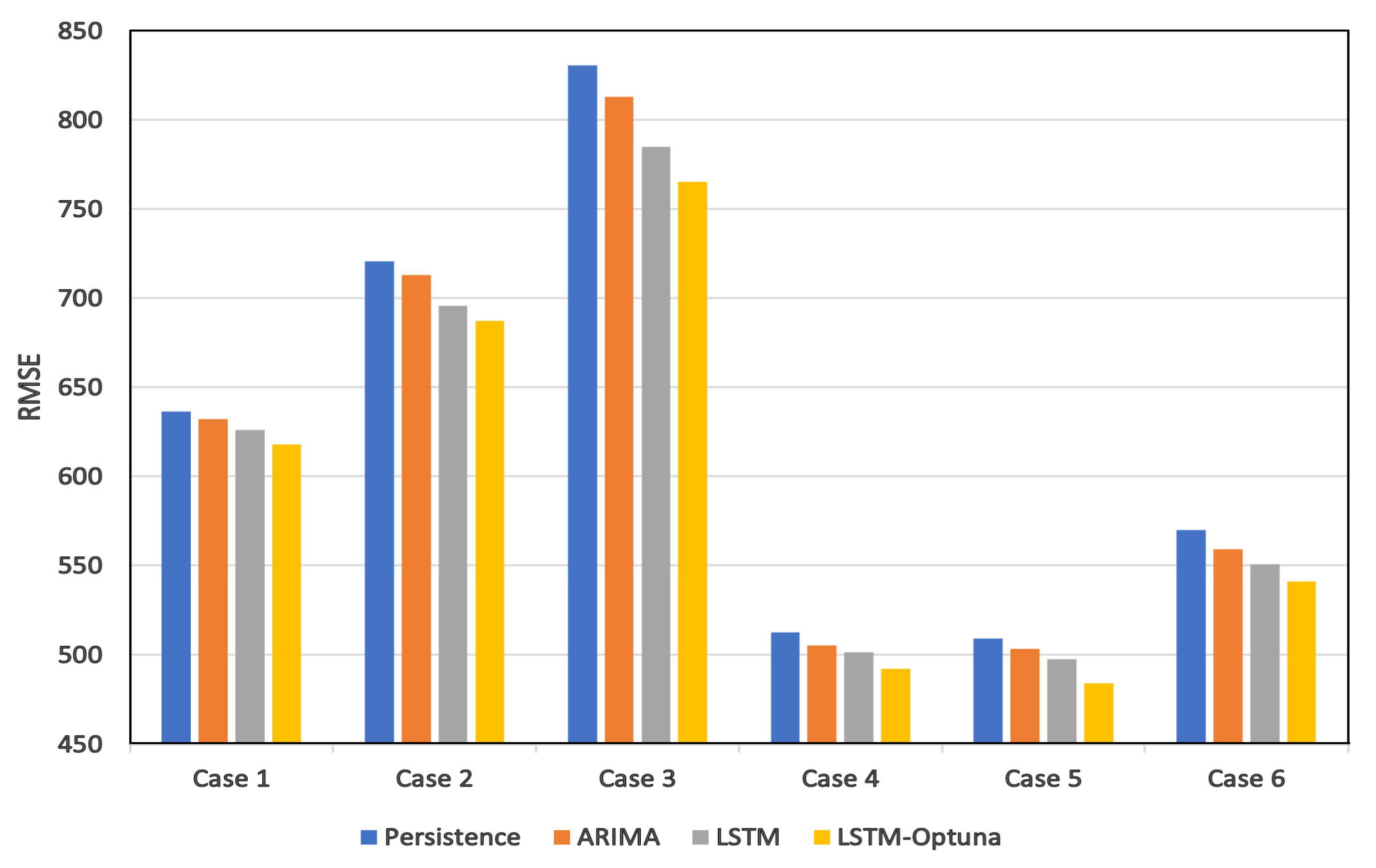
As can be seen in Figure 15, the LSTM model optimised by Optuna can predict more accurately by better learning the wind power’s short-term and long-term dependencies. The diagram illustrated in Figure 16 is plotted to better compare the error levels of the different wind power forecasting methods. It can be recognised from this diagram that the LSTM–Optuna approach follows rules similar to the ARIMA and LSTM–grid models. To achieve a higher prediction accuracy, it is essential to eliminate the outliers and replace the negative power values with the average wind power value.

Building the LSTM models based on the new values of the hyperparameters, as shown in Table 6, improves the prediction accuracy of the LSTM model in a range from 1.22% to 2.65% for different cases of preprocessed data. These accuracy improvements can be seen in

Table 7. A comparison of RMSE, the LSTM–grid search, and LSTM–Optuna methods.

Predictive Model	Case 1	Case 2	Case 3	Case 4	Case 5	Case 6
LSTM tuned by grid search	626	695.8	785	501.5	497.5	550.6
LSTM optimised by Optuna	617.8	687.3	765	492.4	484.3	540.8
Accuracy improvement	1.31%	1.22%	2.55%	1.81%	2.65%	1.78%

.

The results show that the highest accuracy improvement is related to case 5, a case in which negative values were replaced with the mean power value and the outliers were removed through the IF method. A comparison of the required search times to find the best combination of the hyperparameters in LSTM–grid and LSTM–Optuna proves the faster performance of the proposed method, as it spends from 13.79% to 20.59% less time adjusting the model for the most accurate prediction (

Table 8. A comparison of the required tuning time of the LSTM–grid search and LSTM–Optuna methods.

Predictive Model	Case 1	Case 2	Case 3	Case 4	Case 5	Case 6
LSTM tuned by grid search	680	660	290	396	380	340
LSTM optimised by Optuna	540	530	250	340	320	280
Spent time improvement	20.59%	19.70%	13.79%	14.14%	15.79%	17.65%

).

4. Conclusions

This study addresses issues regarding inaccurate wind power prediction using ML approaches. As discussed in the reviewed literature, most previous research applied ML without advanced model optimisation. At the same time, in this paper, a novel concept of Optuna–LSTM is reported to expedite the process of selecting the hyperparameters and tuning the wind power forecasting models. This model not only reduces the time complexity of creating reliable models, but also improves the accuracy of the predictions.

To accurately evaluate the proposed model, SCADA data of an offshore wind turbine was preprocessed by eliminating its negative values and outliers to help find the best preprocessing method. The performance of the proposed forecasting was demonstrated through comparisons with the persistence, ARIMA, and LSTM models, which were already tuned by grid search. This comparison proved the better performance of the proposed model, with a range up to 7.89, 5.9, and 2.65 percent compared to the persistence and conventional grid-search-tuned ARIMA and LSTM models.

This study also highlights the importance of eliminating negative values in the power recordings. The results of this study confirmed that replacing the negative values with the average power value has the most positive effect on the forecasting accuracy. In addition, comparisons between several data cases showed the significant impact of the outlier treatment methods on the forecasting performance. The results proved that removing the outliers by the isolation forest method improves the forecast accuracy compared to the elliptic envelope and OCSVM methods. This novel forecasting method combining the capacity of the LSTM model in the prediction of nonlinearities and the optimisation tool for better tuning the hyperparameters can be used for different time-series-based predictions.