Abstract
The increasing adoption of battery electric vehicles (BEVs) is leading to rising demand for electricity and, thus, leading to new challenges for the energy system and, particularly, the electricity grid. However, there is a broad consensus that the critical factor is not the additional energy demand, but the possible load peaks occurring from many simultaneous charging processes. Hence, sound knowledge about the charging behavior of BEVs and the resulting load profiles is required for a successful and smart integration of BEVs into the energy system. This requires a large amount of empirical data on charging processes and plug-in times, which is still lacking in literature. This paper is based on a comprehensive data set of 2.6 million empirical charging processes and investigates the possibility of identifying different groups of charging processes. For this, a Gaussian mixture model, as well as a k-means clustering approach, are applied and the results validated against synthetic load profiles and the original data. The identified load profiles, the flexibility potential and the charging locations of the clusters are of high relevance for energy system modelers, grid operators, utilities and many more. We identified, in this early market phase of BEVs, a surprisingly high number of opportunity chargers during daytime, as well as switching of users between charging clusters.
1. Introduction
On the one hand, the increasing adoption of battery electric vehicles (BEVs) may pose challenges for the power grid, especially for the low-voltage distribution grid where charging infrastructure for BEVs is typically located [1]. On the other hand, the batteries of BEVs represent a flexibility potential that might become more and more valuable to the energy system in the face of the rollout of renewable energy sources (RES), and the concomitant phase-out of coal and nuclear energy sources [2]. On average, passenger cars are typically parked 23 h a day [3]. Thus, BEVs’ idle times often exceed the charging duration. The resulting flexibility could be used, for example, for postponing or interrupting charging processes, or even feeding back into the grid [4]. By applying controlled charging strategies, charging costs can be reduced or RES usage increased [5].
In order to address future challenges and opportunities associated with BEV adoption from an energy system perspective, distribution system operators (DSOs) need to quantify impacts on grid infrastructure and necessities for grid reinforcement. Therefore, sound forecasts of new load by BEV charging are required. Moreover, new market players of the energy system, such as aggregators, need insights into BEVs’ flexibility potential for determining smart charging or load shifting strategies. Consequently, meaningful data is required for energy systems analyses.
As is today’s best practice, synthetic load profiles or empirical data from field tests are used as input data to energy system models [6,7]. However, with the growing application of BEVs, it is of great significance to have a deep understanding of BEV users’ driving and charging patterns for forecasting both their charging processes and the associated flexibility potential. A detailed insight into the complexity of spatial and temporal charging behavior has enormous significance for the future dimensioning and flexibility assessment of local grids and charging infrastructure or for the use of the flexibility potential of BEVs for the integration of RES.
For this reason, our contribution is twofold. Firstly, we provide insights into real-world charging behavior, based on a comprehensive real-world data set of 2.6 million charging processes in 2019. We particularly focus on the charging process, especially the charging patterns and charging power used, and the plug-in times, i.e., the corresponding charging flexibility potential. The aim is to investigate what insights can be gained using the temporal individual charging behavior of BEVs’ users. For this purpose, we used a two-stage cluster algorithm procedure to identify charging user groups and to derive a standard charging pattern for each user group. We subsequently validated and mapped the BEVs user groups to charging locations, such as at home, at work and in public, supported by synthetic load profiles. In addition, this paper also provides the statistic parameters to replicate and reuse the underlying real-world data set. Thus, on the one hand, the paper allows the drawing of conclusions about real charging behavior and, at the same time, reduces the lack of data, by providing the possibility to replicate the underlying data set, which supports current energy system modelers to consider the load flexibilities of BEVs in much more detail.
To address the above-mentioned research contribution, this work is divided into five parts. Section 2 provides a short overview of the existing literature. Section 3.1 describes the characteristics of the analyzed real-world data set as the basis for the subsequent analyses, as well as describing the necessary data adjustments. Section 3.2 presents the applied methodology of the two cluster algorithms (Gaussian Mixture Model clustering, k-Means clustering). Section 4 describes the results, particularly the assignment of the single charging events to temporal charging clusters and the investigation of the homogeneity of these temporal charging clusters. Based on these temporal charging clusters, we derive user groups and address the associated charging behavior. For validation, we use results from a synthetic load profile generator for BEVs. Section 5 discusses the findings of this work and Section 6 provides the conclusion.
2. Literature Review
The individual charging pattern of BEVs represents a large uncertainty in many analyses due to lack of real-world data [8,9], while individual charging behavior has an influence on numerous aspects. In order to provide grid stability, even with a high penetration of BEVs, DSOs are particularly interested in the individual charging behavior and the resulting load peaks to quantify impacts on grid infrastructure and necessities for grid reinforcement [10]. Ge et al. [11] determine a random based spatial-temporal prediction of BEV charging to obtain more precise insights. Crozier et al. [12] apply a stochastic model based on two different data sources (travel survey data as well as vehicle usage data) to evaluate the BEV charging load and the impacts on the electricity network. One of their key findings is that peak charging demand varies strongly among regions and that representative data is required. Individual charging behavior of BEVs also plays a key role in determining the need for charging infrastructure [13,14]. There is a substantial amount of literature on the prediction of individual charging behavior. One commonly used method is the application of machine learning algorithms to predict charging behavior [15,16]. An alternative method to machine learning algorithms is simulation [17,18]. Zhang et al. [18] investigated charging profiles of electric vehicles presenting a sophisticated simulation method that takes people’s demographic and social characteristics into account. Pagani et al. [17] developed and applied a novel agent-based simulation framework, which takes the charging behavior of individual electric vehicle users as well as the spatial distribution of electric vehicles into account. Knowing the individual charging behavior and the resulting flexibility potential is also crucial for aggregators for defining load shifting strategies. Others, like Sohnen et al. [19], use BEVs’ flexibility potential to evaluate greenhouse gas emissions of BEV charging processes on a dispatch model, based on temporal and spatial effects. Flath et al. [20] analyzed the importance of BEV charging and underlined the possibility of area pricing. This possibility is particularly relevant for real world application if the load flexibilities of EVs are offered and used by energy providers. Deng et al. [21] found that the flexibility provided by BEVs could be used for power reserves and accordingly modeled an BEV aggregator to elaborate this potential of BEVs. Gunkel et al. [22] consider EV flexibility in detail and with respect to the transmission system development. The review paper of Gonzales Venegas et al. [23] goes one-step further and identifies the services which can be provided through BEVs along the value chain. Thereby, possible barriers are classified for active BEV integration. Consequently, meaningful data based on real-world data is required for a successful integration of EVs into the energy power system [24].
Cluster analysis is increasingly applied to smart meter electricity demand data to identify patterns in electricity consumption. The aim is to improve load forecasting, to increase the alignment of demand response programs or to improve the performance in distribution grids [25,26]. Clearly, the scope of the focus in the literature is not only on load profiles for BEVs. In [25] different cluster analysis strategies are examined to identify typical daily heating energy usage profiles. With respect to BEVs, the cluster algorithm is often applied to the charging power profiles. A dataset of hourly load profiles was investigated in [27] and clustering applied to cumulative load profiles to model power consumption during evening peak hours. In [28] the driving and charging behavior of BEVs’ drivers in Shanghai were investigated. They used a machine learning approach as a classifier to analyze the related habitual driver behavior. It is worth emphasizing that clustering is often applied to charging profiles, but not exclusively to the temporal charging behavior. This is the reason why the focus of this contribution is exclusively on the latter.
Up to now, only a few papers have considered empirical data from BEVs to generate BEV load profiles. Among them one is by Schäuble et al. [7], who gained empirical EV load profiles based on three electric mobility studies. The derived charging load profiles gave a realistic understanding of the BEV energy demand. Another data source are the charging stations, where the dataset from Elaad (elaad.nl) is used in literature [29,30]. In the absence of real data, one approach is to use synthetic load profiles derived from the driving behavior of conventional vehicle users, like in Heinz et al. [6]. In this case, real-world data from BEVs’ charging and mobility behavior are lacking. As an alternative, previous studies often rely on numerous assumptions for uncontrolled individual charging behavior [9,31,32,33,34,35,36]. Thus, the individual charging behavior of BEVs plays an important factor in numerous research aspects. Due to the frequent lack of representative real-world data, this paper aims to contribute data and provide insights into the charging behavior based on temporal data of a real-world charging data set of BEV users. At the same time, the possibility of reproducing the underlying dataset is given.
3. Materials and Methods
3.1. Materials
3.1.1. Data Characteristics
The analyzed dataset includes real BEV mobility and charging data from the German vehicle manufacturer BMW. All charging events are associated with the i3 model. The dataset comprises about 2.6 Mio charging processes, each giving information on the location (approximate GPS coordinates), plug-in time, plug-out time, the time of the end of the charging process, starting state-of-charge (SoC) of the battery, ending SoC, and charged energy. The data for our analysis was collected from 1 January 2019 until 31 December 2019 and covers all of Germany and approximately 21,000 BEVs. The identifiers of the individual vehicles are pseudonymized identification numbers so matching the charging activity to the vehicle is possible. The dataset is the largest dataset on charging patterns from a BEV perspective known in literature.
3.1.2. Charging Behavior
The following subchapter presents and discusses the evaluation of the data and the 2.6 million charging processes. Figure 1 shows the distribution of plug-in and plug-out times within a day. It is visible that a larger share of BEVs were connected to the grid in the afternoon and evening hours and the majority of BEVs were unplugged in the morning. It is also noticeable that the frequency of plug-out times was higher than the frequency of plug-in times.
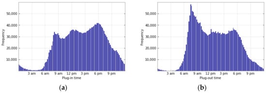
Figure 1.
(a) Distribution of plug-in times over all Germany; (b) Distribution of plug-out times over all Germany.
The average distance driven between two charging processes amounted to 67 km. The remaining battery’s SoC at the beginning of a charging process was 53% on average. The average charging frequency was 96 charging events per BEV over the registration period in the year 2019. Adjusted for the number of weeks in which the vehicle was charged, this corresponded to an average of 3.11 charging processes per week. Therefore, a BMW i3 was charged approximately every two days on average. Compared to Schäuble et al. [7], the charging frequency per BEV in the i3 dataset was higher.
During each charging process, an average of 9.24 kWh of electricity was charged. This meant that, in total, all i3 generated an additional energy demand of 24,595 MWh over one year. The distribution of the additional energy demand of all i3 BEVs for all of Germany in hourly resolution is shown in Figure 2.
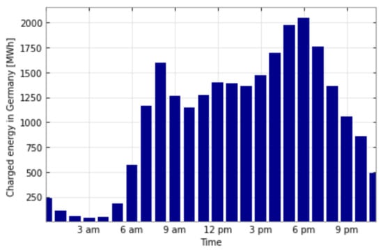
Figure 2.
Charged energy of all i3 BEV for all of Germany in hourly resolution.
For all BEVs, the cumulative average charged energy represents a typical pattern. In order to consider spatial aspects, the plug-in and plug-out times of the different federal states in Germany are shown in Appendix A (cf. Figure A1). The main trend was very similar, but there were differences in the number of BEVs and the related spatial charged energy (cf. Figure A2).
In general, the challenge of integrating BEVs into the power grid lies mainly in the potential load peaks, rather than in the provision of the additional energy. These load peaks depend, in particular, on the individual charging behavior, the charging power used and, thus, the associated simultaneity of the charging processes [1,37].
Therefore, we analyzed the real charging behavior and real charging load profiles of today’s BEV users. Based on the entire i3 dataset, a cumulative, as well as an average (per BEV), charging load profile were generated. The resulting power curves for both all considered charging processes over all of Germany and the per vehicle average are presented in a weekly average in Figure 3a. A classic average load curve could be seen over the period of a week with load peaks in the morning and evening hours. In general, more charging processes took place during the week than on weekends. On average, the load peak for one vehicle was 0.19 kW on weekdays and 0.15 kW on weekends. It is noticeable that there was also a basic charging load during the night hours.
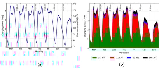
Figure 3.
(a) Average power profile, aggregated (left axis) and proportional (right axis); (b) Average charging profile differentiated by the charging power used.
Since the used charging rate also has an influence on the charging patterns, we considered the used charging power as well. Figure 3b shows the average charging power used over time. Here, the assumption was made that the identification of the used charging rate is possible based on the average charging power of each charging process, calculated by:
for each charging process i. It was noticeable that especially lower charging power rates (3.7 kW and 11 kW) were used for the majority of charging processes.
3.1.3. Flexibility Potential
The flexibility potential of charging processes is of high interest for energy system modelers. Whenever the plug-in time is longer than the charging time a flexibility can be assumed. There are different definitions of load flexibilities of BEVs. In the following we took a conservative approach and defined the shiftable load as follows: If the plug-in duration exceeds the charging time (i.e., there is a temporal flexibility), it is assumed that the load during the temporal flexibility can be increased by the average charging power (cf. Equation (1)) of the charging process. However, if the temporal flexibility is shorter than the charging time only the corresponding fraction is considered and for temporal flexibility this fraction is set to 1. The energy demand during the plug-in period remains the same and the necessary reduced charging at another time is not considered. Hence, other approaches for considering load flexibilities of BEVs, e.g., considering also load shifting potentials between charging events might show significant higher load shifting potentials. Consequently, according to our approach the flexible load is always below the overall load. The average flexibility potential considering the temporal aspects is shown in Figure 4a.
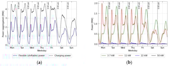
Figure 4.
(a) Average power profile and flexible (shiftable) power; (b) Flexible (shiftable) power per charging power used.
The absolute flexible, shiftable load that could potentially be offered to the grid was quite homogeneous on weekdays and reduced on weekends. The potential flexibility is, of course, always below the load curve, since there are also load processes that do not offer the possibility of shifting the load over time. In the analyzed dataset, about 63% of the charging processes had a flexibility potential. In the remaining charging processes, the vehicles were either not fully charged, i.e., the plug disconnected earlier, or the BEV user terminated the charging process exactly when a SoC of 100% was reached. The temporal flexibility was 8 h on average. It could be seen that there was a comparatively high flexible, shiftable load share, particularly in the morning hours and during the night. BEVs being charged either at the workplace or at home during the night might explain this. Figure 4b shows the flexible, shiftable load in relation to the average charging power used. It was obvious that there was a correlation: the higher the charging power used, the lower the flexible (shiftable) load. This could lead to the conclusion that for numerous charging processes that are associated with a high idle time, lower charging rates are more likely to be used. In addition, the temporal pattern of the shiftable power (which is strongly dependent on the charging power used) can also give an indication of the charging location. In particular, home charging or workplace charging is most likely to be associated with a high idle time and a lower charging rate. This could also be an explanation for the related load peaks.
3.1.4. Data Adjustment
The data involves the date and time of both BEV plug-in and plug-out. These continuous values are difficult to cluster as they do not concentrate on one single day and, therefore, are spread across the whole year. Hence, the dataset was adjusted to enable useful clustering. The first step was based on the assumption that all charging activities started at the same day. The plug-in time was implemented as plug-in time at minute of the day. This approach had the shortcoming that the considered period started at 12 a.m. and ended at 11:59 pm. Early and late plug-in times might not be clustered into one cluster because they lost their spatial proximity. The distribution of the plug-in times is shown in Figure 5. It is visible that the charging activities decreased in early morning hours and increased again later; forming a turning point at around 3 a.m. (red dashed line). To restore the spatial proximity, all charging activities with a plug-in time below this minimum (purple bars) were moved to the right side (blue bars) to continue the time after 12 pm (green dashed line). The data covered by the purple bars was removed to avoid repetition.
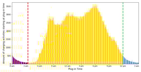
Figure 5.
Distribution of the plug-in times (taking into account data adjustment).
The second feature used for the clustering approach was the plug-in duration. However, the plug-in duration of the different charging activities differs significantly. Some BEVs are plugged-out after a few minutes, while others are plugged-in for several days. Such a dataset repeats itself, creating a cloud of data points for each day (one cloud for the BEVs disconnecting on the same day, one cloud for BEVs disconnecting on the second day, one for the third day, and so on) and making it impossible to gain meaningful clustering results because the clustering might only concentrate on the daily clouds instead of intraday activities. Therefore, we adjusted the data in such a way that all charging activities, which neither ended on the same day nor the next day, ended on the next day, but kept the original plug-out time. This way, two clouds occurred: one for the same day charging activities and one for the overnight charging activities. In addition, the plug-in duration was comparable. The final adjusted data is depicted in Figure 6.
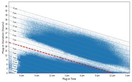
Figure 6.
Final adjusted data depending on plug-in time and plug-in duration, red dashed line represents midnight.
The y-axis covers the plug-in duration and, therefore, added dashed lines depict the plug-out time. Two clouds can be observed. All data points above the midnight line (red dashed line) represented charging activities, which ended on another day; all below represented same-day charging activities.
3.2. Methods
In a first step, we examined the temporal charging behavior and investigated whether a homogeneous charging behavior could be derived and whether conclusions could be drawn about the charging location and charging type. The aim was to examine if BEV user groups, having similar plug-in time and plug-in duration switch, existed, as they would therefore, have similar temporal charging patterns.
3.2.1. Gaussian Mixture Model Clustering
Due to the sheer amount of data points, it was difficult to recognize clusters immediately, making it difficult to choose the clustering approach right away. Therefore, in a first step the distribution of the data was analyzed, shown in Figure 7.
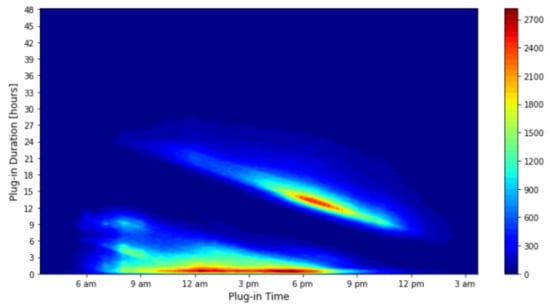
Figure 7.
Density distribution of the final dataset.
The high concentration of the data is a common indicator for the application of density-based approaches. In addition, the clustering approach needs to perform well with large datasets regarding computation time and memory limitations [38]. Based on these limiting factors, the Gaussian Mixture Model (GMM) clustering was applied.
The GMM clustering is an unsupervised approach, which decomposes complex distribution of a database into K Gaussian distributions , so called components, with a mean µk, covariance Covk and weight πk each [39]; each distribution represents a cluster.
Before choosing the final number of clusters, the clustering approach was conducted with several different numbers of clusters and the Aikaki Information Criterion [40] and the Bayesian Information Criterion [41] were calculated. Both criteria helped to assess the fit of the developed model, and to avoid overfitting of the data. Based on the analysis of these two criteria, the GMM clustering was conducted with seven clusters.
3.2.2. K-Means Clustering
To analyze the charging behavior, only BEV users with more than 20 charging activities were chosen for the second clustering approach. The number of total charging activities and the charging activities during each of the above-derived temporal charging clusters were counted, and the share of charging activities for each cluster for the user was calculated. These shares for each user built the base for the next clustering step.
The unsupervised k-means clustering approach was used to derive the different temporal behavior clusters [42]. K-Means is a simple and commonly used clustering approach for behavior analysis. Some examples where k-means is applied for driving pattern analysis are Fugiglando et al. [43] and Dardas et al. [44]. The aim of k-means clustering is to find cluster centers and assign each data point of the data set to a cluster center. The assignment of data point to a cluster center is conducted via binary variable . Each data point can be assigned to only one cluster center. The k-means approach finds values for and to minimize the sum of all distances between the data points and their cluster centers. This function is sometimes called distortion measure [39]:
Due to the seven clusters in the GMM clustering, the dataset of the k-means clustering has seven dimensions. To examine if all these dimensions are necessary for the k-means clustering, the dimensions were normalized and the number of dimensions reduced by a subsequent principal component analysis [43]. The final number of clusters was chosen by applying the elbow technique for different numbers of clusters [45]. Based on this analysis, five clusters were chosen.
4. Results
Based on the methodological approach described in the previous Section 3.2.1, seven temporal charging clusters were identified. In the following, we examine the seven clusters (cf. Figure 8) in more detail and validate them with the aim of trying to categorize them.
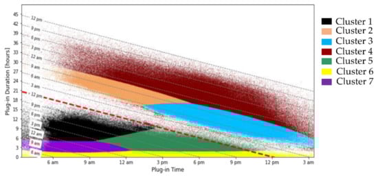
Figure 8.
Related Clusters to the GMM-Clustering, red dashed line represents midnight.
The already high number of seven clusters showed that the data was too complex to be described by a few Gaussian distributions. Moreover, the following two main agglomerations of charging incidents, identified in Figure 7, were somewhat surprising: there were many overnight chargers, who plugged-in between 6 pm and 9 pm, and another hot spot seemed to be a huge group of opportunity chargers during the day, who stood out because of the short charging times during the daytime. This latter group has not been considered in most energy systems models. Besides these two hot spots, there was still a broad range of other charging incidents. Consequently, the GMM clustering split the overnight (Clusters 2, 3, and 4), as well as the daytime (Clusters 1, 5, 6, and 7), chargers into different groups. The mean, weight, and covariance of each cluster and the total number of samples in each cluster are depicted in Table A1 in the Appendix B. The evaluation of the identified charging clusters is shown in Table 1. The associated graphs can be found in Appendix B (Figure A3, Figure A4, Figure A5, Figure A6, Figure A7, Figure A8 and Figure A9). There, the distribution of the plug-in times, the plug-out times and the distribution of the plug-in durations, as well as the average load profile (considering the charging powers used), are shown.

Table 1.
Characteristics of the temporal charging clusters.
As shown in Table 1 and in Figure A3, Figure A4, Figure A5, Figure A6, Figure A7, Figure A8 and Figure A9 (in Appendix B), the temporal charging clusters differed with regard to the temporal charging characteristics, such as plug-in time, plug-out time and plug-in duration. Differences could also be identified with regard to the charging power used, as well as the load peaks and the temporal flexibility potential. It should be noted that the effective flexibility potential was higher due to the data adjustment, since the charging processes with more than 48 h were not included. The number of charging processes within a cluster also influenced the peak load.
Cluster 1 and Cluster 7 were characterized by plugging-in during the morning and plugging-out after a medium plug-in duration. The charging events included in Cluster 5 were charging processes that began in the afternoon and had a medium plug-in duration. Cluster 6 contained the charging processes that took place during the day and had a rather short plug-in duration. Clusters 1, 5, 6, and 7 were united by the fact that they were plugged-in and plugged-out on the same day. Clusters 2 to 4 did not have plug-in and plug-out times on the same day (represented by the red dashed line in Figure 8) and, therefore, had a significantly longer plug-in duration. The temporal flexibility potential and the charging power used also varied significantly per temporal charging cluster (see Table 1). Interestingly, while temporal charging clusters with low flexibility potential tended to be associated with charging processes that had used high charging power (cf. Cluster 6), high temporal flexibilities were mainly associated with charging processes with low charging power (cf. Clusters 2, 3, and 4).
Based on the clustering results, we analyzed how homogeneous the charging behavior of BEV users was. The results of this assessment showed that BEV users did not behave homogeneously by charging their BEVs during similar hours and for similar durations. This finding contradicted the classification of BEV users into fixed user groups.
5. Discussion
The identified temporal charging clusters are not very useful for energy system modelers as the characteristics of users and charging locations are missing. With this additional information the modelers would be able to allocate the right charging patterns to the observed users or charging. We, therefore, added two further analyses: first, we tried to identify whether users switch between clusters and, second, we compared our empirically based findings with currently applied load curves, which are usually based on empirical data from conventional vehicles. If these two load curves coincide, current load curves can be further applied in energy systems modeling.
For identifying switching car users between clusters, we applied a k-means clustering with the original user IDs (cf. Appendix C). Surprisingly, there was quite frequent change between charging clusters. This might come from the free charging opportunities at attractive parking places. The k-means clustering came up with 5 user groups which did not seem as homogenous than expected. Nevertheless, they were analyzed in further detail (cf. Appendix C).
For comparing our load patterns with existing approaches in literature, which base their charging patterns on plug-in assumptions and empirical mobility data from conventional car usage, we applied the MobiFlex tool (Heinz et al., 2018) for generating synthetic load patterns (cf. Appendix D). The comparison between the two charging curves were surprisingly similar. Only the frequent opportunity charging during the daytime was underrepresented in the synthetic load profiles by the MobiFlex tool. Furthermore, the switching between the different charging incidents could not be found in the synthetic load profiles. However, in our analyses we found that the resulting charging load patterns at the different charging locations, such as home, workplace, public or fast charging, showed surprising similar results. As these results are of high interest for all energy system modelers, we plotted the resulting load curves from the MobiFlex tool (cf. Figure A16, Figure A17, Figure A18 and Figure A19) and provide the underlying csv files in the Supplementary Materials.
Even though our dataset was very comprehensive compared to other current available data from BEVs, our approach relied only on the technical data, and user data was not available. Furthermore, all data came from only one specific BEV, the i3 by BMW, and all charging was undertaken in an early market phase of BEVs. Nevertheless, the dataset delivers significant insights to current literature.
6. Conclusions
Within the scope of the analysis, the charging behavior of an empirical dataset of real-world charging data, containing approximately 21,000 battery-electric vehicles and about 2.6 million charging processes over a period of one year, was investigated.
In summary, our results show that, based on the exclusive consideration of individual temporal charging data, conclusions could be drawn about battery-electric vehicle user groups and related charging patterns and flexible (shiftable) load. Two main findings could be highlighted: in this early market phase, a surprisingly high number of opportunity chargers during the day, as well as switching users between charging clusters, were identified. Moreover, an estimation of the charging location is possible. We provided resulting load curves, which can be used in energy system models to consider the load shifting potential of battery electric vehicles in more detail.
For future research, further factors of the charging process should be considered in addition to the temporal aspects. For example, the charging power, the amount of energy charged and the charging frequency also play a decisive role. The spatial distribution should also be taken into account in future studies. It should also be emphasized that the underlying real-world data set can be reproduced, based on our analysis, and can, thus, be used for further scientific studies, such as investigating numerous research questions with regard to battery-electric vehicles and to support the successful sustainable integration of electric vehicles into the energy system.
Supplementary Materials
The following supporting information can be downloaded at: https://www.mdpi.com/article/10.3390/en15186575/s1.
Author Contributions
A.M.: Conceptualization, methodology, software, validation, data curation, writing—original draft preparation, writing—review and editing, visualization. U.L.: Methodology, software, validation, writing—original draft preparation, writing—review and editing, visualization. S.R.: Validation, writing—original draft preparation, writing—review and editing, visualization. K.S.: Writing—original draft preparation, writing—review and editing, supervision. P.J.: Data acquisition, writing—review and editing. All authors have read and agreed to the published version of the manuscript.
Funding
This paper resulted from the project Scientific Evaluation of Energy Services–Wissenschaftliche Begleitung von Geschäftsmodellen bei der BMW Group.
Data Availability Statement
Data is contained within Supplementary Materials. The data for Figure A16, Figure A17, Figure A18 and Figure A19 in this study are available in the Supplementary Materials.
Acknowledgments
We highly acknowledge the very good collaboration with BMW Group. We thank all project partners for their valuable comments and discussions, which have made a major impact on this paper. We acknowledge support by the KIT-Publication Fund of the Karlsruhe Institute of Technology.
Conflicts of Interest
The authors declare no conflict of interest. The funders had no role in the design of the study; in the collection, analyses, or interpretation of data; in the writing of the manuscript, or in the decision to publish the results.
Appendix A. Charging Behavioral Data
- Plug-in and plug-out times per Federal State
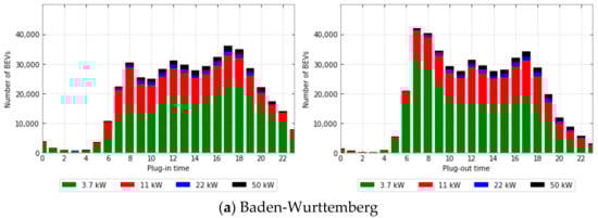
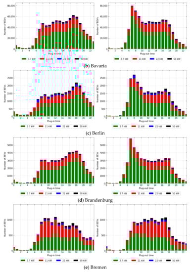
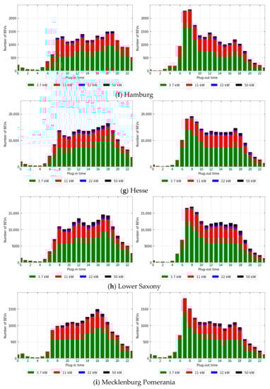
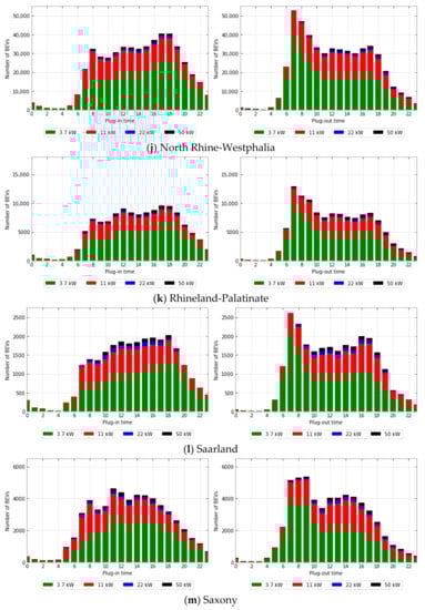
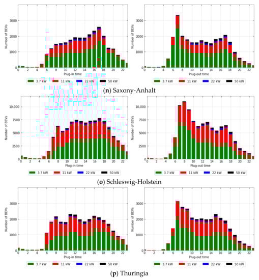
Figure A1.
(a–p) Plug-in and plug-out times taking into account the charging power used per state.
- Charged energy per Federal State [MWh]
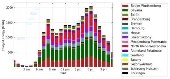
Figure A2.
Charged energy of all i3 BEVs per Federal State.
Appendix B. Further Descriptive Statistical Indicators
- The mean, weight and covariance of each cluster and the total number of samples in each cluster.
Table A1.
The mean, weight and covariance of each cluster and the total number of samples in each temporal charging cluster.
Table A1.
The mean, weight and covariance of each cluster and the total number of samples in each temporal charging cluster.
| Temporal Charging Cluster | Mean µ | Covariance Matrix ∑ | Weight π | Number of Samples in Cluster |
|---|---|---|---|---|
| Cluster 1 | 0.1000 | 252,370 | ||
| Cluster 2 | 0.0902 | 215,767 | ||
| Cluster 3 | 0.2229 | 660,084 | ||
| Cluster 4 | 0.1184 | 272,415 | ||
| Cluster 5 | 0.1620 | 396,360 | ||
| Cluster 6 | 0.2071 | 617,763 | ||
| Cluster 7 | 0.0995 | 247,508 |
- Charging characteristics for the identified temporal charging clusters
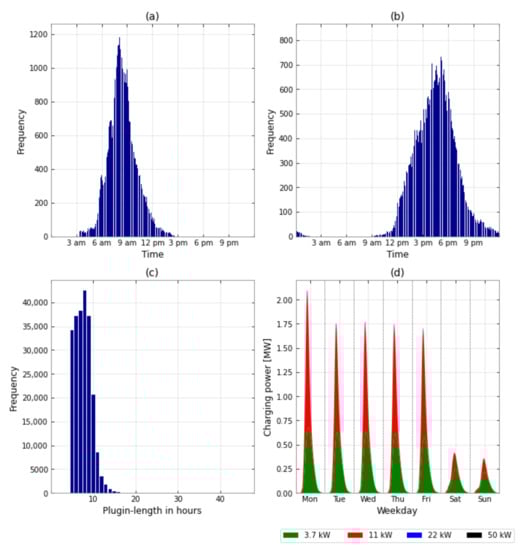
Figure A3.
Charging characteristics of temporal charging cluster 1: (a) Frequency of different plug-in times; (b) Frequency of different plug-out times; (c) Frequency of different plug-in lengths; (d) Charging power used.
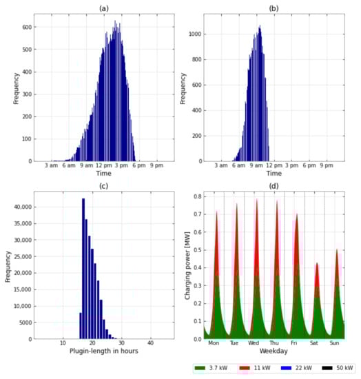
Figure A4.
Charging characteristics of temporal charging cluster 2: (a) Frequency of different plug-in times; (b) Frequency of different plug-out times; (c) Frequency of different plug-in lengths; (d) Charging power used.
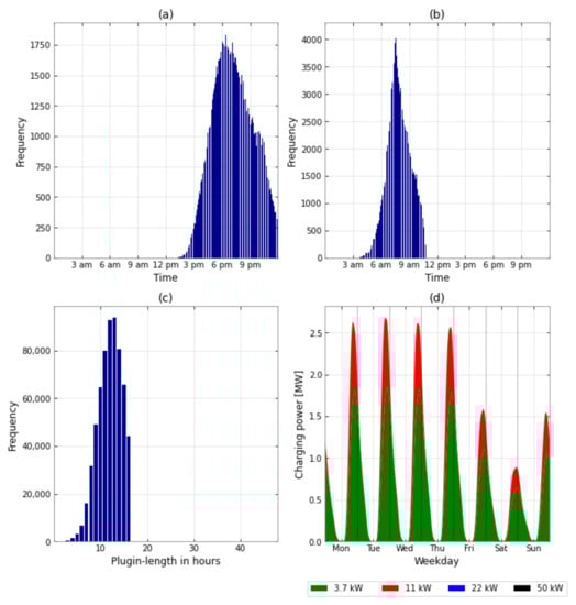
Figure A5.
Charging characteristics of temporal charging cluster 3: (a) Frequency of different plug-in times; (b) Frequency of different plug-out times; (c) Frequency of different plug-in lengths; (d) Charging power used.
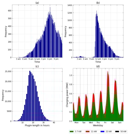
Figure A6.
Charging characteristics of temporal charging cluster 4: (a) Frequency of different plug-in times; (b) Frequency of different plug-out times; (c) Frequency of different plug-in lengths; (d) Charging power used.
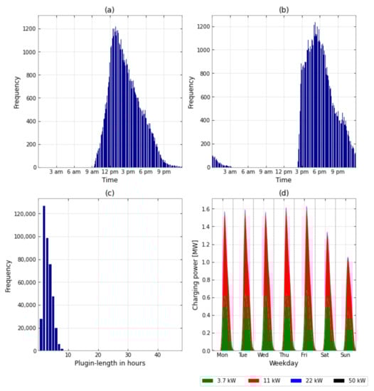
Figure A7.
Charging characteristics of temporal charging cluster 5: (a) Frequency of different plug-in times; (b) Frequency of different plug-out times; (c) Frequency of different plug-in lengths; (d) Charging power used.
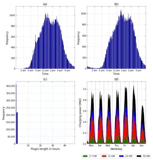
Figure A8.
Charging characteristics of temporal charging cluster 6: (a) Frequency of different plug-in times; (b) Frequency of different plug-out times; (c) Frequency of different plug-in lengths; (d) Charging power used.
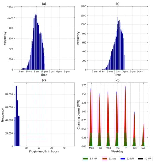
Figure A9.
Charging characteristics of temporal charging cluster 7: (a) Frequency of different plug-in times; (b) Frequency of different plug-out times; (c) Frequency of different plug-in lengths; (d) Charging power used.
Appendix C. Clustering of User Groups
To cluster users into charging groups, we applied the k-Means clustering approach (Section 3.2.2). The resulting five user groups are composed of the shares of the differently used temporal charging clusters (cf. Figure 8) and are shown in Figure A10.
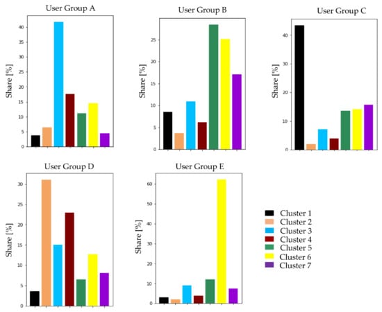
Figure A10.
Related Clusters to the k-Means Clustering.
In the following, the five identified user groups were analyzed taking into account the load pattern, and the charging power used, as well as the flexible (shiftable) power. User Group A included 7830 BEV users and 1,056,623 charging activities. This user group was characterized by the fact that the main charging activities took place mainly at night, with a strong focus on the afternoon/evening plug-in times and the morning unplugging times. In addition, there were short- and medium-term activities. The load pattern, as well as the associated charging power and the flexible shiftable power, are shown in Figure A11. The afternoon/evening plug-in times can also be seen in the load pattern, which were particularly evident in the afternoon/evening hours. The charging activities mainly took place with smaller charging powers (3.7 kW and 11 kW). Occasionally, charging powers of 22 kW or 50 kW were also in use and could be assigned to short- or medium-term charging activities.
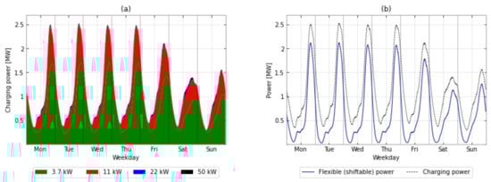
Figure A11.
(a) User Group A: Charging power profile as a function of the assumed charging power used; (b) User Group A: Relation between the charging power profile and the associated flexible (shiftable) power.
User Group B consisted of 5232 BEV users and 661,683 charging activities with a strong focus on short- and medium-term charging activities. The load pattern and the flexible (shiftable) load are pictured in Figure A12. The peak tended to be in the morning hours and the most used charging power in this user group was 11 kW. User Group B had a medium flexible power shifting potential.
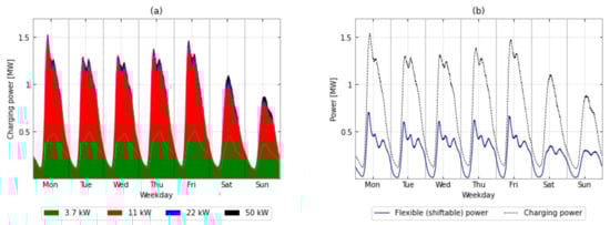
Figure A12.
(a) User Group B: Charging power profile as a function of the assumed charging power used; (b) User Group B: Relation between the charging power profile and the associated flexible (shiftable) power.
User Group C had 1900 BEV users and 240,897 charging activities, which were typified by a high share of medium-term charging activities, which mainly started in the morning hours (cf. Figure A13). Other short- and medium-term activities also occurred in this charging type. This composition of the temporal charging clusters was also reflected in the load pattern. In this user group, the load peaks were found in the morning hours and had a high temporal density. Interestingly, the extreme load peaks were only observed on weekdays. The most frequently used charging power in this user group was 3.7 kW and 11 kW during the week; charging processes with higher charging powers could also be assigned at the weekend. In general, this user group had a high potential for flexible power, which was particularly concentrated in the morning hours.
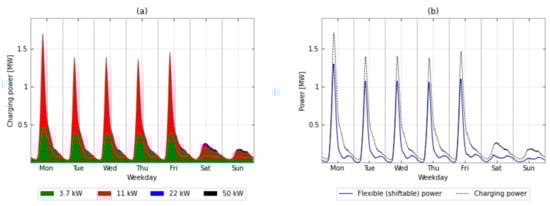
Figure A13.
(a) User Group C: Charging power profile as a function of the assumed charging power used; (b) User Group C: Relation between the charging power profile and the associated flexible (shiftable) power.
2994 BEV users and 328,562 charging activities characterized User Group D. A high share of the charging activities took place over the night but without concentration on evening plug-ins and morning plug-outs. Furthermore, some short-term activities took place. Nevertheless, the occurrence of the charging process was more widely distributed throughout the day. In Figure A14, it can be seen that here, too, the focus was on the lower charging powers (3.7 kW and 11 kW) and that there were decisive differences between weekday and weekend. In general, there was a very high flexible (shiftable) load in this user group.
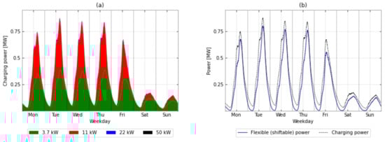
Figure A14.
(a) User Group D: Charging power profile as a function of the assumed charging power used; (b) User Group D: Relation between the charging power profile and the associated flexible (shiftable) power.
User Group E included 2683 BEV users and 329,998 charging activities. The users charged, in particular, by means of short-term charging processes during the daytime hours. What was remarkable here was the share of charging processes that were carried out with a high charging power of 11 kW, 22 kW and 50 kW (cf. Figure A15). The charging behavior of this user group was quite uniform over the course of a week; only on Sundays were there slightly fewer charging processes on average. This user group had only a very low flexible power shifting potential.
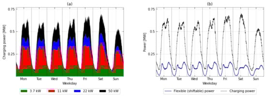
Figure A15.
(a) User Group E: Charging power profile as a function of the assumed charging power used; (b) User Group E: Relation between the charging power profile and the associated flexible (shiftable) power.
The five user groups described in detail above were compared to each other. The user groups differed in terms of their average load profile and the load peak, as well as the most frequently used charging power with regard to the flexible (shiftable) load.
The load profiles resulted from the composition of the temporal charging cluster shares (cf. Figure 8) and, therefore, led to very different load profiles of the different user groups. The flexibility resulting from the idle time when the BEV was connected to the grid, but the charging process was already completed, also showed differences. Obviously, the number of BEVs and charging processes also had a decisive influence. In particular, user group A had the highest load peaks, which were higher on weekdays than on weekends. User Group C showed a peak especially on weekday mornings and User Group E showed a constant load curve over a week, in average. The charging pattern could be explained by the shares of charging processes in the temporal charging clusters. While User Groups A and D offered a high temporal flexibility potential, a significantly higher load could be shifted in User Group A. The focus of the shiftable load in User Group D was also mainly on weekdays. In terms of temporal flexibility, User Groups B and C were similar, but they differed in terms of the shiftable load. While User Group B also had a share of shiftable loads at the weekend, the share of shiftable loads in User Group C was particularly during the week. User Group E generally had a very low flexibility potential in terms of time and quantity.
Appendix D. Comparison with Synthetically Generated Charging Profiles
In this section, we analyze the hypothesis that the identified temporal charging clusters and, thus, the identified user groups could be associated to charging locations. Therefore, the MobiFlex simulation model that generates synthetic BEV charging profiles based on empirical and representative driving data of conventional passenger vehicles, was applied. For further details, please refer to Ecke et al. (2019), Ried (2020), and Heinz et al. (2018).
The following assumptions were made for the generation of the synthetic load profiles. These assumptions were based on the obtained temporal charging clusters (Figure 8 and Table 1). Further input data of the MobiFlex model can be found in Table A2.
- Temporal chargings in Clusters 2 and 3 represented home charging activities because of overnight charging events, relatively long charging durations and a peak in plug-out-time during the morning hours (commuters).
- Temporal chargings in Clusters 1 and 7 represented workplace charging, because they covered charging events with plug-in time in the morning and the plug-out occurring on the same day.
- Temporal chargings in Cluster 6 represented public charging, because of short plug-in durations.
Table A2.
Further input data for the MobiFlex model.
Table A2.
Further input data for the MobiFlex model.
| Parameter | Value |
|---|---|
| Average battery capacity (calculated using the analyzed dataset) | 23.4 kWh |
| Average energy consumption | 17 kWh/100 km |
| Charging efficiency | 90% |
| Probability of charging power at home | |
| 3.7 kW | 76.2% |
| 11 kW | 23.7% |
| 22 kW | 0.1% |
| 50 kW | 0.0% |
| Probability of charging power at work | |
| 3.7 kW | 57.0% |
| 11 kW | 42.1% |
| 22 kW | 0.8% |
| 50 kW | 0.1% |
| Probability of charging power at public | |
| 3.7 kW | 38.4% |
| 11 kW | 36.0% |
| 22 kW | 9.3% |
| 50 kW | 16.3% |
The probabilities of charging power at the different locations were calculated based on charging power per charging event in the respective charging location. In the following analysis, four model configurations were carried out: (1) Home charging only, (2) Public charging only, (3) Workplace charging only, (4) Both home and workplace charging. Different user groups were not pre-determined in advance. Instead, the MobiFlex model was applied to the full dataset of all approximately 2300 passenger cars. Those vehicles that could be replaced by BEVs under the given assumptions then determined the total charging power. For comparability reasons, the load profiles are shown on a per vehicle basis. The charging profiles generated are shown below (Figure A16, Figure A17, Figure A18 and Figure A19). These reflect the load profile on the one hand and the charging power used on the other. In order to draw conclusions about the charging location, they were compared with the user groups obtained by the k-means clustering.
In the first model configuration, only the possibility of home charging was considered. The probabilities for the charging power used can be taken from Table A2. The resulting charging pattern is shown in Figure A16.
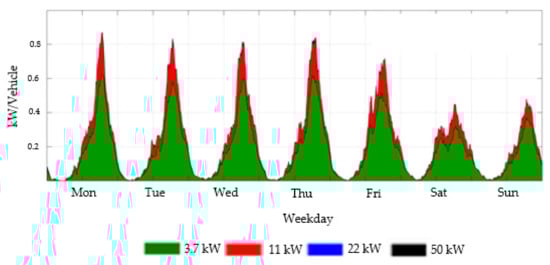
Figure A16.
Charging patterns for uncontrolled charging for “home charging”.
The charging pattern of this configuration, the load peaks in the evening and the used charging power showed a congruence with User Group A (cf. Figure A11a).
The second configuration examined the case where only public charging was possible. The resulting charging pattern (Figure A17) showed similarities with User Group E (Figure A15a). There were two peaks on weekdays and one main peak on Saturday morning. However, the MobiFlex model did not show any overnight charging.
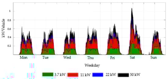
Figure A17.
Charging Patterns for uncontrolled charging for “public charging”.
When charging is only possible at the workplace, MobiFlex generated the charging pattern shown in Figure A18, which had similarities to User Group C (cf. Figure A13a). Here, the load peak in the morning hours was particularly characteristic.
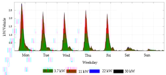
Figure A18.
Charging Patterns for uncontrolled charging for “workplace charging”.
If both home charging and workplace charging were included in the charging processes, it resulted in the load profile illustrated in Figure A19. However, this charging pattern did not resemble any of the above user groups.
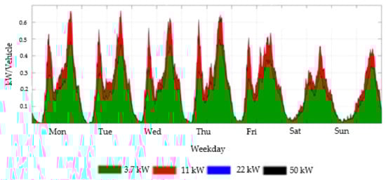
Figure A19.
Charging Patterns for uncontrolled charging for both “home and workplace charging”.
This might lead to the hypothesis that the temporal charging in Clusters 2 and 3 mainly covered home charging, temporal charging in Clusters 1 and 7 mainly workplace charging, and in Cluster 6 public charging. Since the user groups were composed of the shares of the temporal charging clusters (see Figure A10), User Group A might be rather home chargers, User Group C workplace chargers, and User Group E mostly public short-term chargers. Thus, possible charging locations could be assigned to the three user groups.
References
- Jochem, P.; Märtz, A.; Wang, Z. How might the German distribution grid cope with 100% market share of PEV? In Proceedings of the 31th International Electric Vehicle Symposium, Kobe, Japan, 30 September–3 October 2018. [Google Scholar]
- Xu, L.; Yilmaz, H.; Wang, Z.; Poganietz, W.-R.; Jochem, P. Greenhouse gas emissions of electric vehicles in Europe considering different charging strategies. Transp. Res. Part D: Transp. Environ. 2020, 87, 102534. [Google Scholar] [CrossRef]
- Ecke, L.; Chlond, B.; Magdolen, M.; Eisenmann, C.; Hilgert, T.; Vortisch, P. Deutsches Mobilitätspanel (MOP)—Wissenschaftliche Begleitung und Auswertungen Bericht 2017/2018: Alltagsmobilität und Fahrleistung; Karlsruher Institut für Technologie, Institut für Verkehrswesen: Karlsruhe, Germany, 2019. [Google Scholar]
- Ried, S. Gesteuertes Laden von Elektrofahrzeugen in Verteilnetzen mit hoher Einspeisung erneuerbarer Energien—Ein Beitrag zur Kopplung von Elektrizitäts- und Verkehrssektor; KIT Scientific Publishing: Karlsruhe, Germany, 2021. [Google Scholar] [CrossRef]
- Seddig, K.; Jochem, P.; Fichtner, W. Two-stage stochastic optimization for cost-minimal charging of electric vehicles at public charging stations with photovoltaics. Appl. Energy 2019, 242, 769–781. [Google Scholar] [CrossRef]
- Heinz, D. Erstellung und Auswertung Repräsentativer Mobilitäts- und Ladeprofile für Elektrofahrzeuge in Deutschland; Karlsruhe Institute of Technology (KIT), Institute for Industrial Production (IIP): Karlsruhe, Germany, 2018. [Google Scholar]
- Schäuble, J.; Kaschub, T.; Ensslen, A.; Jochem, P.; Fichtner, W. Generating electric vehicle load profiles from empirical data of three EV fleets in Southwest Germany. J. Clean. Prod. 2017, 150, 253–266. [Google Scholar] [CrossRef]
- ElNozahy, M.S.; Salama, M.M.A. A Comprehensive Study of the Impacts of PHEVs on Residential Distribution Networks. IEEE Trans. Sustain. Energy 2014, 5, 332–342. [Google Scholar] [CrossRef]
- Kong, P.-Y.; Karagiannidis, G.K. Charging Schemes for Plug-In Hybrid Electric Vehicles in Smart Grid: A Survey. IEEE Access 2016, 4, 6846–6875. [Google Scholar] [CrossRef]
- Knezović, K.; Marinelli, M.; Zecchino, A.; Andersen, P.B.; Træholt, C. Supporting involvement of electric vehicles in distribution grids: Lowering the barriers for a proactive integration. Energy 2017, 134, 458–468. [Google Scholar] [CrossRef]
- Ge, X.; Shi, L.; Fu, Y.; Muyeen, S.M.; Zhang, Z.; He, H. Data-driven spatial-temporal prediction of electric vehicle load profile considering charging behavior. Electr. Power Syst. Res. 2020, 187, 106469. [Google Scholar] [CrossRef]
- Crozier, C.; Morstyn, T.; McCulloch, M. Capturing diversity in electric vehicle charging behaviour for network capacity estimation. Transp. Res. Part D Transp. Environ. 2021, 93, 102762. [Google Scholar] [CrossRef]
- Chakraborty, D.; Bunch, D.S.; Lee, J.H.; Tal, G. Demand drivers for charging infrastructure-charging behavior of plug-in electric vehicle commuters. Transp. Res. Part D Transp. Environ. 2019, 76, 255–272. [Google Scholar] [CrossRef]
- Kavianipour, M.; Fakhrmoosavi, F.; Singh, H.; Ghamami, M.; Zockaie, A.; Ouyang, Y.; Jackson, R. Electric vehicle fast charging infrastructure planning in urban networks considering daily travel and charging behavior. Transp. Res. Part D Transp. Environ. 2021, 93, 102769. [Google Scholar] [CrossRef]
- Chung, Y.-W.; Khaki, B.; Li, T.; Chu, C.; Gadh, R. Ensemble machine learning-based algorithm for electric vehicle user behavior prediction. Appl. Energy 2019, 254, 113732. [Google Scholar] [CrossRef]
- Huber, J.; Dann, D.; Weinhardt, C. Probabilistic forecasts of time and energy flexibility in battery electric vehicle charging. Appl. Energy 2020, 262, 114525. [Google Scholar] [CrossRef]
- Pagani, M.; Korosec, W.; Chokani, N.; Abhari, R. User behaviour and electric vehicle charging infrastructure: An agent-based model assessment. Appl. Energy 2019, 254, 113680. [Google Scholar] [CrossRef]
- Zhang, J.; Yan, J.; Liu, Y.; Zhang, H.; Lv, G. Daily electric vehicle charging load profiles considering demographics of vehicle users. Appl. Energy 2020, 274, 115063. [Google Scholar] [CrossRef]
- Sohnen, J.; Fan, Y.; Ogden, J.; Yang, C. A network-based dispatch model for evaluating the spatial and temporal effects of plug-in electric vehicle charging on GHG emissions. Transp. Res. Part D Transp. Environ. 2015, 38, 80–93. [Google Scholar] [CrossRef]
- Flath, C.M.; Ilg, J.P.; Gottwalt, S.; Schmeck, H.; Weinhardt, C. Improving Electric Vehicle Charging Coordination Through Area Pricing. Transp. Sci. 2014, 48, 619–634. [Google Scholar] [CrossRef]
- Deng, R.; Xiang, Y.; Huo, D.; Liu, Y.; Huang, Y.; Huang, C.; Liu, J. Exploring flexibility of electric vehicle aggregators as energy reserve. Electr. Power Syst. Res. 2020, 184, 106305. [Google Scholar] [CrossRef]
- Gunkel, P.A.; Bergaentzlé, C.; Jensen, I.G.; Scheller, F. From passive to active: Flexibility from electric vehicles in the context of transmission system development. Appl. Energy 2020, 277, 115526. [Google Scholar] [CrossRef]
- Venegas, F.G.; Petit, M.; Perez, Y. Active integration of electric vehicles into distribution grids: Barriers and frameworks for flexibility services. Renew. Sustain. Energy Rev. 2021, 145, 111060. [Google Scholar] [CrossRef]
- Das, H.S.; Rahman, M.M.; Li, S.; Tan, C.W. Electric vehicles standards, charging infrastructure, and impact on grid integration: A technological review. Renew. Sustain. Energy Rev. 2020, 120, 109618. [Google Scholar] [CrossRef]
- Ma, Z.; Yan, R.; Nord, N. A variation focused cluster analysis strategy to identify typical daily heating load profiles of higher education buildings. Energy 2017, 134, 90–102. [Google Scholar] [CrossRef]
- Xiang, Y.; Hong, J.; Yang, Z.; Wang, Y.; Huang, Y.; Zhang, X.; Chai, Y.; Yao, H. Slope-Based Shape Cluster Method for Smart Metering Load Profiles. IEEE Trans. Smart Grid 2020, 11, 1809–1811. [Google Scholar] [CrossRef]
- Satre-Meloy, A.; Diakonova, M.; Grünewald, P. Cluster analysis and prediction of residential peak demand profiles using occupant activity data. Appl. Energy 2020, 260, 114246. [Google Scholar] [CrossRef]
- Yang, J.; Dong, J.; Zhang, Q.; Liu, Z.; Wang, W. An Investigation of Battery Electric Vehicle Driving and Charging Behaviors Using Vehicle Usage Data Collected in Shanghai, China. Transp. Res. Rec. J. Transp. Res. Board 2018, 2672, 20–30. [Google Scholar] [CrossRef]
- Amara-Ouali, Y.; Goude, Y.; Massart, P.; Poggi, J.-M.; Yan, H. A Review of Electric Vehicle Load Open Data and Models. Energies 2021, 14, 2233. [Google Scholar] [CrossRef]
- Helmus, J.; Spoelstra, J.; Refa, N.; Lees, M.; Hoed, R.V.D. Assessment of public charging infrastructure push and pull rollout strategies: The case of the Netherlands. Energy Policy 2018, 121, 35–47. [Google Scholar] [CrossRef]
- Gadea, A.; Marinelli, M.; Zecchino, A. A Market Framework for Enabling Electric Vehicles Flexibility Procurement at the Distribution Level Considering Grid Constraints. In Proceedings of the 2018 Power Systems Computation Conference, Dublin, Ireland, 11–15 June 2018; pp. 1–7. [Google Scholar]
- Li, M.; Lenzen, M. How many electric vehicles can the current Australian electricity grid support? Int. J. Electr. Power Energy Syst. 2020, 117, 105586. [Google Scholar] [CrossRef]
- Fernandez, L.P.; Roman, T.G.S.; Cossent, R.; Domingo, C.M.; Frias, P. Assessment of the Impact of Plug-in Electric Vehicles on Distribution Networks. IEEE Trans. Power Syst. 2011, 26, 206–213. [Google Scholar] [CrossRef]
- Plagowski, P.; Saprykin, A.; Chokani, N.; Shokrollah-Abhari, R. Impact of electric vehicle charging—An agent-based approach. IET Gener. Transm. Distrib. 2021, 12, 6033. [Google Scholar] [CrossRef]
- Shafiee, S.; Rastegar, M.; Fotuhi-Firuzabad, M. Impacts of controlled and uncontrolled PHEV charging on distribution systems. In Proceedings of the 9th IET International Conference on Advances in Power System Control, Operation and Management (APSCOM 2012), Hong Kong, China, 18–21 November 2012; Institution of Engineering and Technology: London, UK; p. 154. [Google Scholar]
- Shahidinejad, S.; Filizadeh, S.; Bibeau, E. Profile of Charging Load on the Grid Due to Plug-in Vehicles. IEEE Trans. Smart Grid 2012, 3, 135–141. [Google Scholar] [CrossRef]
- Märtz, A.; Held, L.; Wirth, J.; Jochem, P.; Suriyah, M.; Leibfried, T. Development of a Tool for the Determination of Simultaneity Factors in PEV Charging Processes. In Proceedings of the 3rd E-Mobility Power System Integration Symposium, Dublin, Ireland, 14 October 2019. [Google Scholar]
- Patel, E.; Kushwaha, D.S. Clustering Cloud Workloads: K-Means vs Gaussian Mixture Model. Procedia Comput. Sci. 2020, 171, 158–167. [Google Scholar] [CrossRef]
- Bishop, C.M.; Nasrabadi, N.M. Pattern Recognition and Machine Learning; Springer: New York, NY, USA, 2006; Volume 4. [Google Scholar]
- De Leeuw, J. Introduction to Akaike (1973) Information Theory and an Extension of the Maximum Likelihood Principle. In Foundations and Basic Theory, 2nd ed.; Kotz, S., Ed.; Springer: New York, NY, USA; Berlin, Germany, 1993; pp. 599–609. [Google Scholar]
- Schwarz, G. Estimating the Dimension of a Model. Ann. Stat. 1978, 6, 461–464. [Google Scholar] [CrossRef]
- Lloyd, S.P. Least squares quantization in PCM. IEEE Trans. Inf. Theory 1982, 28, 129–137. [Google Scholar] [CrossRef]
- Fugiglando, U.; Massaro, E.; Santi, P.; Milardo, S.; Abida, K.; Stahlmann, R.; Netter, F.; Ratti, C. Driving Behavior Analysis through CAN Bus Data in an Uncontrolled Environment. IEEE Trans. Intell. Transp. Syst. 2019, 20, 737–748. [Google Scholar] [CrossRef]
- Dardas, A.Z.; Williams, A.; Scott, D. Carer-employees’ travel behaviour: Assisted-transport in time and space. J. Transp. Geogr. 2020, 82, 102558. [Google Scholar] [CrossRef]
- Syakur, M.A.; Khotimah, B.K.; Rochman, E.M.S.; Satoto, B.D. Integration K-Means Clustering Method and Elbow Method for Identification of The Best Customer Profile Cluster. IOP Conf. Series Mater. Sci. Eng. 2018, 336, 012017. [Google Scholar] [CrossRef] [Green Version]
Publisher’s Note: MDPI stays neutral with regard to jurisdictional claims in published maps and institutional affiliations. |
© 2022 by the authors. Licensee MDPI, Basel, Switzerland. This article is an open access article distributed under the terms and conditions of the Creative Commons Attribution (CC BY) license (https://creativecommons.org/licenses/by/4.0/).