
Transport Efficiency of a Homogeneous Gaseous Substance in the Presence of Positive and Negative Gaseous Sources of Mass and Momentum

Abstract
:1. Introduction
2. Considered Flow Cases and Calculation Results
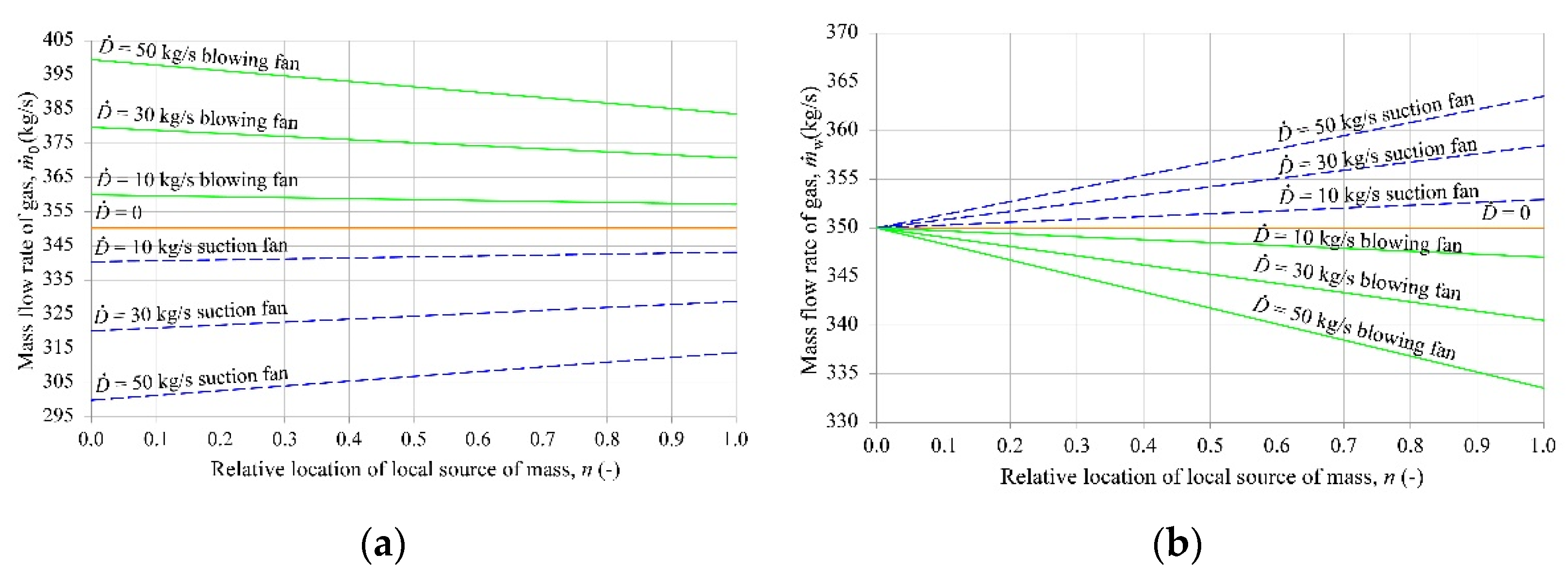
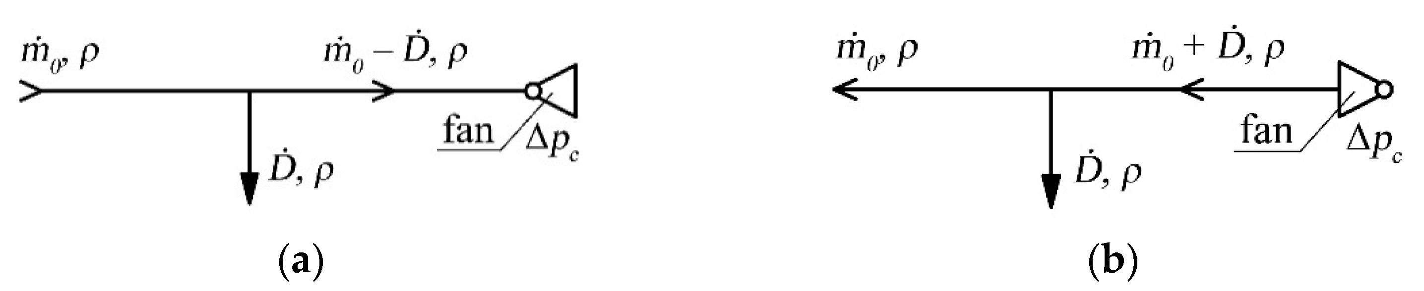
2.1. Case 1
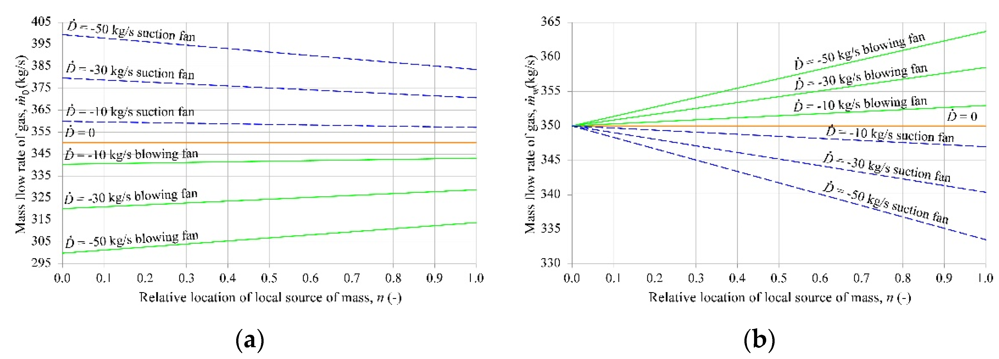
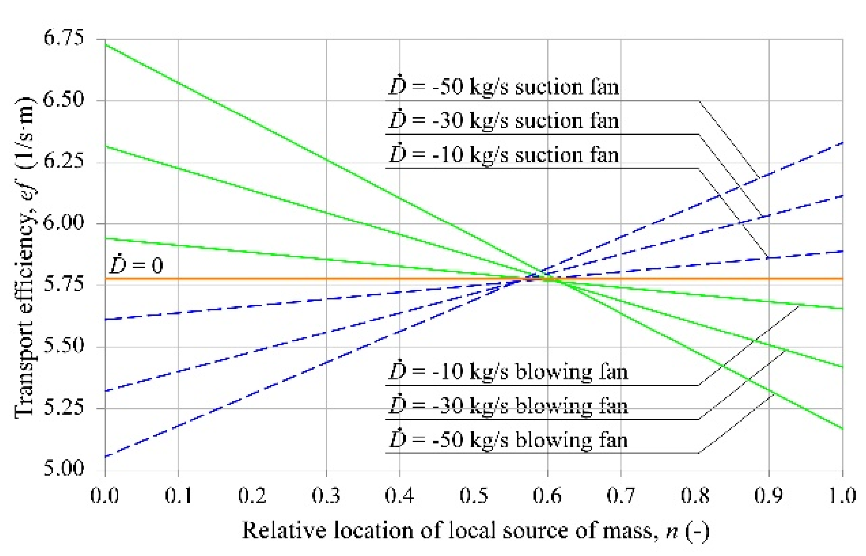
2.2. Case 2
3. Conclusions
Author Contributions
Funding
Institutional Review Board Statement
Informed Consent Statement
Data Availability Statement
Conflicts of Interest
Nomenclature
| hydraulic diameter of the duct, m | |
| internal source of mass flow, kg/(m·s) | |
| mass flow rate of local source of mass, kg/s | |
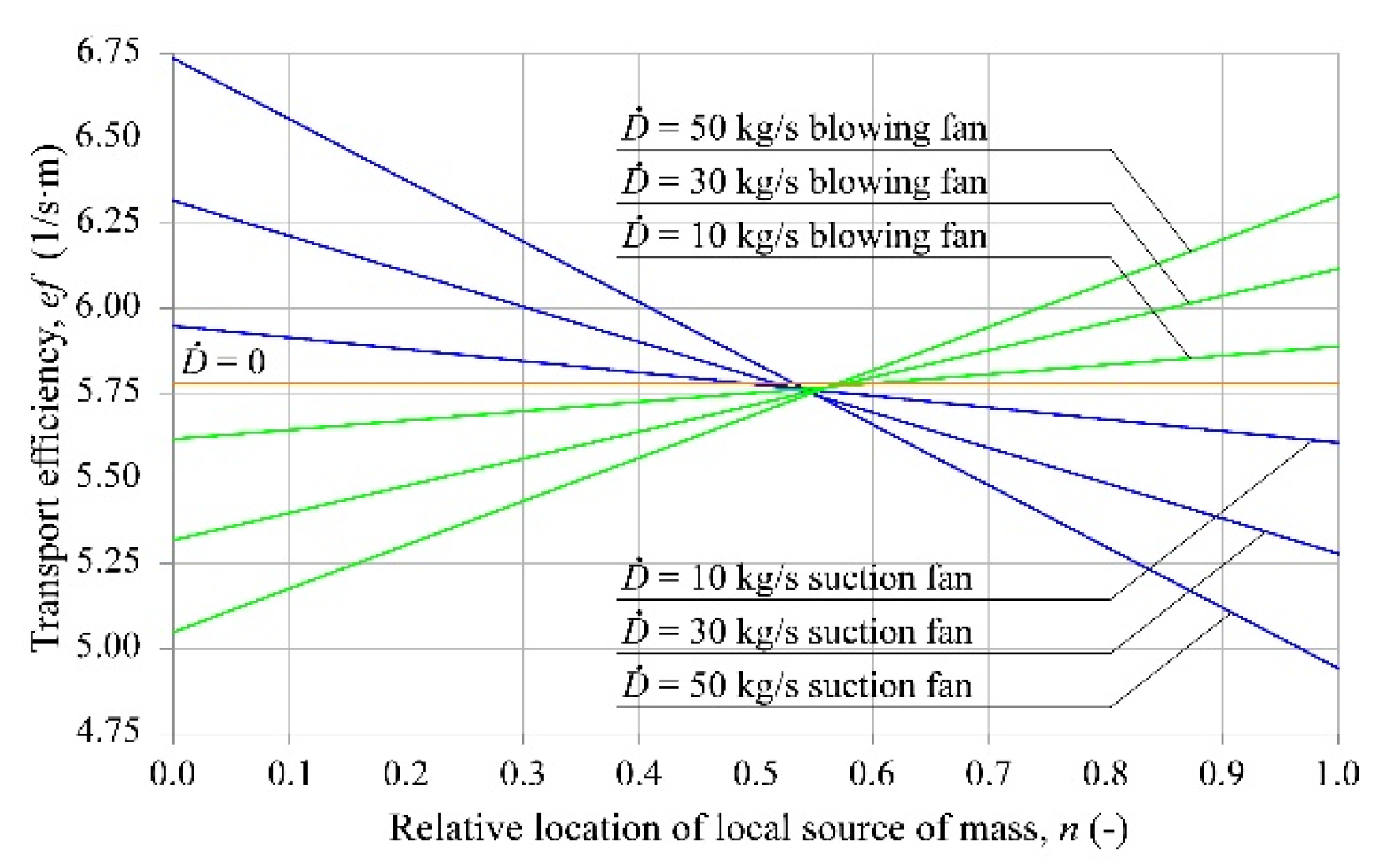
| energy efficiency for the observed medium’s flow, (m·s)−1 | |
| cross-sectional area of the duct, m2 | |
| gravity, m/s2 | |
| hydraulic gradient per unit (dimensionless) caused by the linear resistance of the duct, | |
| duct length, m | |
| mass flow rate of fluid, kg/s | |
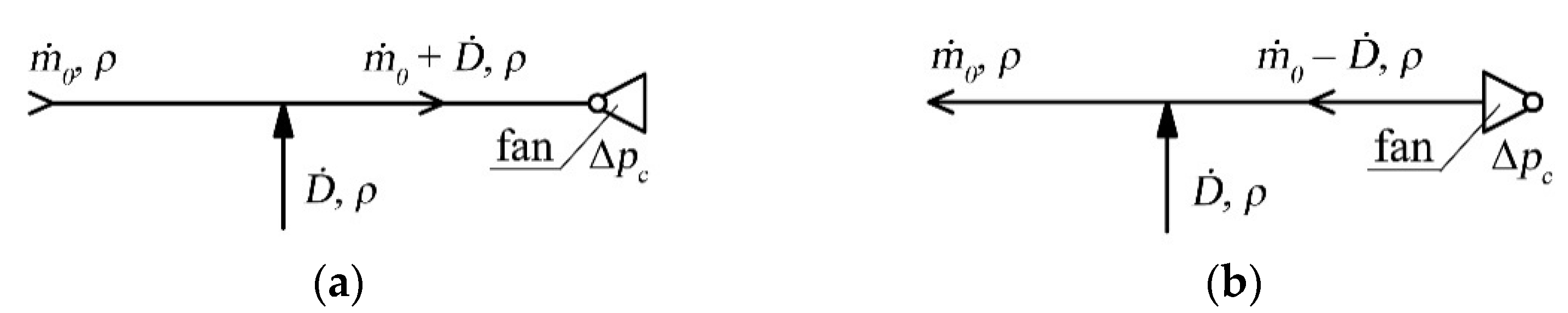
| mass flow rate of gas entering the duct, the opposite end of which features a mechanical suction source (mass flow rate of gas leaving the duct, the opposite end of which features a mechanical suction source), kg/s | |
| mass flow rate of gas flowing through the fan, kg/s | |
| ratio of the drag of the duct section from its entry to the point where the local source of mass is located and the drag of the entire duct () | |
| absolute static pressure of the fluid, Pa | |
| cross-sectional circumference of the duct, m | |
| distributed drag per unit of the duct (a straight duct), kg/m8 | |
| specific drag, Ns2/m8 or kg/m7 | |
| R* | specific drag of the duct, 1/(kg·m) |
| duct’s equivalent drag per unit, kg/m8 | |
| flow velocity of incoming mass aligned with the mass flow direction in the duct, m/s | |
| volumetric flow rate of the flowing fluid, m3/s | |
| loss of mechanical energy (total head), N/m2 | |
| static-pressure drop at local resistance at a point with the coordinate , N/m2 | |
| x | distance, m |
| z | above-sea-level spot height of a given duct location, m |
| Greek symbols | |
| distributed-resistance coefficient of the duct, kg/m3 | |
| Dirac delta function distribution, 1/m | |
| total pressure increase for a working fan, N/m2 | |
| dimensionless distributed resistance coefficient of the duct, | |
| average gas velocity, m/s | |
| density, kg/m3 | |
| time, s | |
References
- Pawiński, J.; Roszkowski, J.; Strzemiński, J. Przewietrzanie Kopalń; Śląskie Wydawnictwo Techniczne: Katowice, Poland, 1995. [Google Scholar]
- Ptaszyński, B. Charakterystyka przepływowa przewodu transportującego różne media. In Proceedings of the 8 Szkoła Aerologii Górniczej. Sekcja Aerologii Górniczej: Nowoczesne Metody Zwalczania Zagrożeń Aerologicznych w Podziemnych Wyrobiskach Górniczych, Jaworze, Poland, 13–16 October 2015. [Google Scholar]
- Wacławik, J. Mechanika Płynów i Termodynamika; Wydawnictwo AGH: Kraków, Poland, 1993. [Google Scholar]
- Dziurzyński, W.; Krach, A.; Pałka, T. Airflow Sensitivity Assessment Based on Underground Mine Ventilation Systems Modeling. Energies 2017, 10, 1451. [Google Scholar] [CrossRef]
- Zmrhal, V.; Boháč, J. Pressure loss of flexible ventilation ducts for residential ventilation: Absolute roughness and compression effect. J. Build. Eng. 2021, 44, 103320. [Google Scholar] [CrossRef]
- Sleiti, A.K.; Zhai, J.; Idem, S. Computational fluid dynamics to predict duct fitting losses: Challenges and opportunities. HVAC&R Res. 2013, 19, 2–9. [Google Scholar] [CrossRef]
- Kodali, C.; Idem, S. Modeling flow and pressure distributions in multi-branch light-commercial duct systems. Sci. Technol. Built Environ. 2021, 27, 240–252. [Google Scholar] [CrossRef]
- Semin, M.A.; Levin, L.Y. Stability of air flows in mine ventilation networks. Process Saf. Environ. Prot. 2019, 124, 167–171. [Google Scholar] [CrossRef]
- Onder, M.; Cevik, E. Statistical model for the volume rate reaching the end of ventilation duct. Tunn. Undergr. Space Technol. 2008, 23, 179–184. [Google Scholar] [CrossRef]
- Auld, G. An estimation of fan performance for leaky ventilation ducts. Tunn. Undergr. Space Technol. 2004, 19, 539–549. [Google Scholar] [CrossRef]
- Akhtar, S.; Kumral, M.; Sasmito, A.P. Correlating variability of the leakage characteristics with the hydraulic performance of an auxiliary ventilation system. Build. Environ. 2017, 121, 200–214. [Google Scholar] [CrossRef]
- McPherson, M.J. Subsurface Ventilation and Environmental Engineering; Chapman&Hall: London, UK, 1992. [Google Scholar]
- Wacławik, J. Wentylacja Kopalń, Tom I, II; Wydawnictwo AGH: Krakow, Poland, 2010. [Google Scholar]
- Yamaguchi, H. Engineering Fluid Mechanics; Springer Netherlands: Dordrecht, The Netherlands, 2010. [Google Scholar]
- Bergander, M.J. Fluid Mechanics Volume 1. Basic Principles; AGH University of Science and Technology Press: Krakow, Poland, 2010. [Google Scholar]


Publisher’s Note: MDPI stays neutral with regard to jurisdictional claims in published maps and institutional affiliations. |
© 2022 by the authors. Licensee MDPI, Basel, Switzerland. This article is an open access article distributed under the terms and conditions of the Creative Commons Attribution (CC BY) license (https://creativecommons.org/licenses/by/4.0/).
Share and Cite
Ptaszyński, B.; Kuczera, Z.; Życzkowski, P.; Łuczak, R. Transport Efficiency of a Homogeneous Gaseous Substance in the Presence of Positive and Negative Gaseous Sources of Mass and Momentum. Energies 2022, 15, 6376. https://doi.org/10.3390/en15176376
Ptaszyński B, Kuczera Z, Życzkowski P, Łuczak R. Transport Efficiency of a Homogeneous Gaseous Substance in the Presence of Positive and Negative Gaseous Sources of Mass and Momentum. Energies. 2022; 15(17):6376. https://doi.org/10.3390/en15176376
Chicago/Turabian StylePtaszyński, Bogusław, Zbigniew Kuczera, Piotr Życzkowski, and Rafał Łuczak. 2022. "Transport Efficiency of a Homogeneous Gaseous Substance in the Presence of Positive and Negative Gaseous Sources of Mass and Momentum" Energies 15, no. 17: 6376. https://doi.org/10.3390/en15176376
APA StylePtaszyński, B., Kuczera, Z., Życzkowski, P., & Łuczak, R. (2022). Transport Efficiency of a Homogeneous Gaseous Substance in the Presence of Positive and Negative Gaseous Sources of Mass and Momentum. Energies, 15(17), 6376. https://doi.org/10.3390/en15176376