Joint History Matching of Multiple Types of Field Data in a 3D Field-Scale Case Study ^†

Abstract

This work presents an ensemble-based workflow to simultaneously assimilate multiple types of field data in a proper and consistent manner. The aim of using multiple field datasets is to improve the reliability of estimated reservoir models and avoid the underestimation of uncertainties. The proposed framework is based on an integrated history matching workflow, in which reservoir models are conditioned simultaneously on production, tracer and 4D seismic data with the help of three advanced techniques: adaptive localization (for better uncertainty quantification), weight adjustment (for balancing the influence of different types of field data), and sparse data representation (for handling big datasets). The integrated workflow is successfully implemented and tested in a 3D benchmark case with a set of comparison studies (with and without tracer data). The findings of this study indicate that joint history matching using production, tracer and 4D seismic data results in better estimated reservoir models and improved forecast performance. Moreover, the integrated workflow is flexible, and can be extended to incorporate more types of field data for further performance improvement. As such, the findings of this study can help to achieve a better understanding of the impacts of multiple datasets on history matching performance, and the proposed integrated workflow could serve as a useful tool for real field case studies in general.

1. Introduction

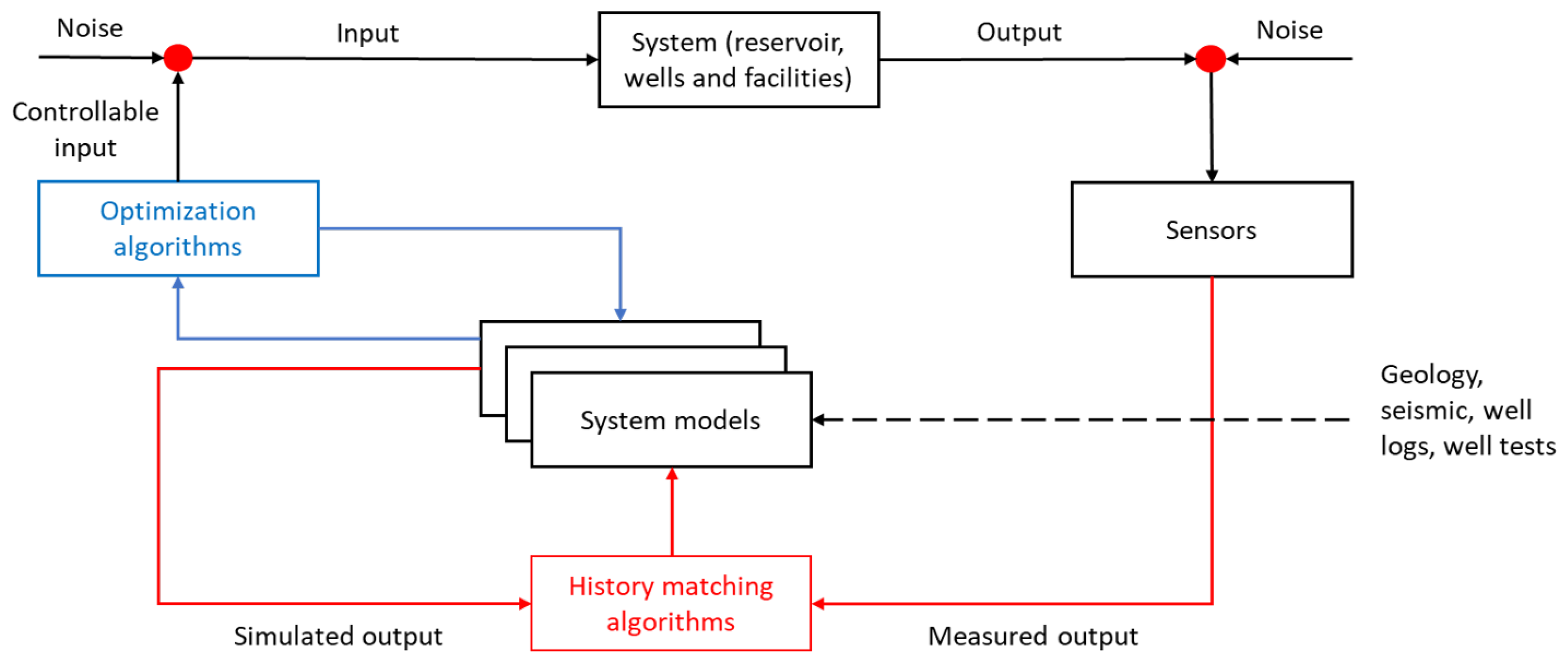
In the petroleum industry, reservoir simulation plays an important role for the decision-making process of oil field developments, where a common practice is to apply a closed-loop workflow [1] to develop and manage reservoir performance under different scenarios and conditions, as shown in Figure 1. This type of simulation is commonly used to predict and/or optimize future oil, gas, and water productions in a field (referred to as system). However, uncertainties and simplifications are involved in the construction of reservoir models (system models), due to the lack of sufficient information in, e.g., geology, seismic data, well logs and tests. Consequently, reservoir parameters (e.g., permeability, and porosity) are not accurately obtained, which makes reservoir models uncertain for production forecasts, and the corresponding decision-making process unreliable for reservoir management. In order to improve the reliability of production forecasts, one needs to condition reservoir models on sensored field datasets, through a process known as history matching in the literature. In this way, the estimated parameters of reservoir models can generate simulated outputs that are as close as possible to the field datasets.

In a standard history matching process, the field data used to estimate uncertain reservoir model parameters are well production data, which include bottom hole pressure, and oil, gas, and water rates. These kinds of measurements are frequent in time and relatively cheap in terms of acquisition cost, but their usefulness is often somewhat insufficient for the purpose of reducing uncertainties in production forecasts, due to their limited spatial coverage of the reservoir [2,3]. In addition to production data, other types of field data, e.g., inter-well tracer and 4D seismic data, can be used as complementary sources of information to further reduce the uncertainties-hence improve the reliability-of reservoir models, which constitutes the focus of the current study.

Inter-well tracer test (IWTT) has been proven as an efficient technology to obtain information of fluid dynamics, well-to-well communication, and heterogeneities such as fractures and flow barriers (for a review of tracer studies see [4]). In the tracer technology, inert compounds (e.g., radioactive, chemical, or natural tracers) are used to label water or gas from specific wells, and trace fluid movements as the tracer flow moves through the reservoir together with the injection fluid. After the first breakthrough in a producer, IWTT provides a reliable and definite information of a well-to-well communication.

On the other hand, 4D seismic data contain much more information in space, especially about pressure and fluid saturation changes. Therefore, seismic data provide another useful source of information for understanding reservoir behavior, and identifying zones of remaining oils [5]. When used in combination with production and tracer data, they could further improve the qualities of reservoir models through history matching, and thus generate more reliable production forecasts for better decision making.

Despite the appealing features of tracer and 4D seismic data, they are still often qualitatively employed for reservoir monitoring and management in the petroleum industry, but are relatively less used in a quantitative way, due to various reasons arising from both theoretical understandings and practical applications to jointly match both types of field data in a coherent way. Tracer has been incorporated into history matching by a few authors [3,5,6,7,8,9,10]. Meanwhile, recently, several authors have demonstrated the benefits of incorporating seismic data into a history matching process [2,11,12,13,14,15]. Nevertheless, methodologies for jointly history matching production, tracer, and 4D seismic data have not been previously studied in the literature yet. Thus, there is a potential to include both tracer and 4D seismic data into a history matching workflow to further reduce the uncertainties and improve the reliability of reservoir models.

In the literature, there are different schools of approaches to tackling history matching problems. For instance, history matching can be formulated as a conventional minimization problem, in which an iterative algorithm is used, in combination with certain geoestatistical modelling methods [16,17], to find the best matched model(s). Among the iterative history matching algorithms, ensemble-based methods have received immense attention in the petroleum industry, for their convenience in implementation and computational efficiency to handle big models and big data sets when compared to other conventional methods [18]. For instance, the ensemble Kalman filter (EnKF) introduced by [19] was initially extensively used for history matching problems [20,21]. As a sequential algorithm, however, the EnKF requires frequent simulator restarts, which may cause significant additional simulation time and other practical challenges (e.g., more prone to failed reservoir simulations) [22]. To avoid these noticed issues, ensemble smoother (ES) [23] and its iterative versions [24,25,26,27,28] can be adopted instead. In comparison to the EnKF, ES and iterative ES (IES) do not need simulator restarts and have less model variables to update during history matching, and are practically easier to implement than the EnKF for history matching problems. In addition, various numerical results (e.g., [25,26]) indicate that the IES tends to perform better than the EnKF and the ES. As a result, currently, the IES appears to be among the state-of-the-art approaches to history matching problems, and is thus adopted in the current work.

The recent developments of ensemble-based history matching algorithms make the quantitative use of multiple field data sets easier and faster. Despite this technological advancement, to the best of our knowledge, there are no existing studies demonstrating the benefits of simultaneously assimilating production, tracer and 4D seismic data into reservoir models through an ensemble-based history matching algorithm. As a main focus (and contribution) of this study, our primary objective is to demonstrate the benefits of assimilating tracer and 4D seismic data (in addition to production) in an integrated, ensemble-based history matching workflow, through a 3D field-scale case study.

This work is organized as follows: First, we provide details of the integrated ensemble-based history matching workflow, which includes the formulation of an IES algorithm and a correlation-based adaptive localization scheme. Second, we apply the history matching workflow to a 3D field case, the Brugge benchmark [29], and examine the performance of the proposed workflow. Finally, we conclude the work with some technical discussions and our future research plan.

2. Ensemble-Based History Matching Workflow

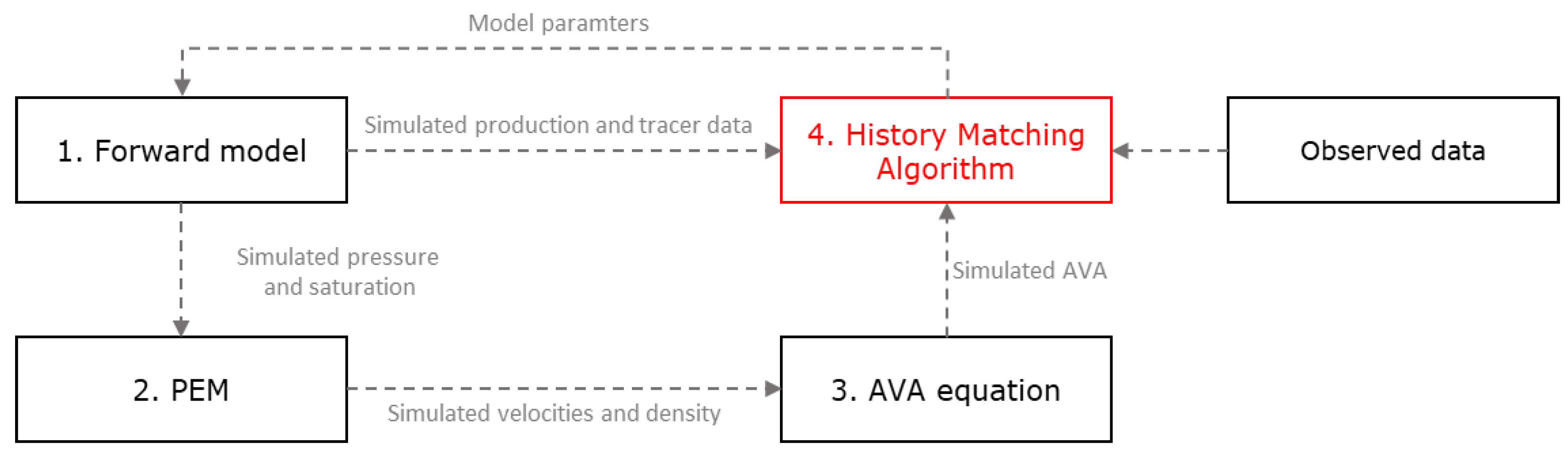
Figure 2 illustrates the flowchart of the integrated history matching workflow using multiple types of field data. To formulate the history matching problem, we assume there is a forward simulator $\mathbf{g}$ (e.g., a numerical reservoir and/or seismic simulator) which outputs a $N_{\mathrm{d}}$-dimensional vector containing the simulated data ${\mathbf{d}}^{sim}$, given a $N_{\mathrm{m}}$-dimensional vector of reservoir model $\mathbf{m}$ as the input:

$${\mathbf{d}}^{sim}=\mathbf{g}\left(\mathbf{m}\right).$$

(1)

Note that, in Step 1 of Figure 2, the forward simulator generates an ensemble of simulated production and tracer data, with an ensemble of input reservoir models, while the forward seismic simulator produces an ensemble of simulated amplitude-versus-angle (AVA) data, with the associated petro-elastic model (PEM) and AVA at Steps 2 and 3, respectively, based on the simulated pressure and saturation profiles from the forward reservoir simulator, and the simulated velocities and density profiles from the PEM, respectively. The formulation of the forward seismic simulator is presented in Appendix A.

Furthermore, we have the observed (field) data ${\mathbf{d}}^o$ which are obtained through the following noisy observation system:

$${\mathbf{d}}^o=\mathbf{g}\left({\mathbf{m}}_{\mathrm{true}}\right)+\delta ,$$

(2)

where ${\mathbf{m}}_{\mathrm{true}}$ stands for the ground-truth model (unknown in a real reservoir), $\mathbf{g}\left({\mathbf{m}}_{\mathrm{true}}\right)$ for the true output of the forward model, and $\delta$ for a $N_{\mathrm{d}}$-dimensional vector of contamination noise that may be present in the course of field data acquisition, which are assumed to follow a multivariate Gaussian distribution with zero mean and covariance (referred to as measurement error-covariance matrix) represented by ${\mathbf{C}}_{\mathrm{d}}$, i.e., $\delta \sim N(\mathbf{0},{\mathbf{C}}_{\mathrm{d}})$.

With the above observation system, in Step 4 of Figure 2, a history matching algorithm is then adopted to find one or multiple reservoir models $\mathbf{m}$ whose simulated output $\mathbf{g}\left(\mathbf{m}\right)$ matches the observed data ${\mathbf{d}}^o$ reasonably well. In practice, when the size of the observed data is much smaller than of the reservoir model parameters (e.g., $N_{\mathrm{d}}\ll Nm$), history matching is an under-determined and high-dimensional inverse problem, which makes the history matching problem challenging, in the sense that in principle there could exist an infinite number of reservoir models matching the observed data equally well (non-uniqueness), due to the large degree of freedom (DOF) from the model side [30].

To mitigate this problem, one can either introduce a certain regularization term in the form of a least-square problem, or increase the number of field data in history matching [3]. Here we consider both aforementioned ideas, by including both a regularization term into a relevant cost function (cf. Equation (3)), and multiple types of field data into history matching.

Practical challenges may arise with multiple types of field data in history matching. For instance, different from production and tracer data, 4D seismic data are less frequent in time, but with a much larger size. Thus, when assimilating large datasets, computational issues regarding storage memory and CPU time may emerge. Meanwhile, large datasets could have a dominant influence on model updates in history matching. Moreover, with large field datasets, ensemble-based history matching methods are often prone to ensemble collapse (meaning that an ensemble of reservoir models also collapses into a single one, with few varieties among reservoir models), and thus tend to under-estimate model uncertainties [15]. Our approaches to handling the aforementioned issues include conducting a sparse representation of seismic data for dimension reduction, adjusting the relative weights among different types of field data to balance their influence on history matching, and conducting correlation-based localization to mitigate the issue of under-estimated uncertainties, which will be elaborated in Section 3 later.

2.1. Iterative Ensemble Smoother Based on a Regularized Levenburg–Marquardt Algorithm

As history matching problems are typically non-linear, a certain iterative method is needed to deal with the non-linearity. In the current work, we adopt one such method, called iterative ensemble smoother based on the regularized Levenburg–Marquardt algorithm (IES-RLM) [26].

In IES-RLM, one aims to find an ensemble ${\mathcal{M}}^{i+1}\equiv {\left\{{\mathbf{m}}_j^{i+1}\right\}}_{j=1}^{N_e}$ of reservoir models that approximately minimizes a nonlinear-least-squares (NLS) cost function, as follows:

$$\begin{array}{cc}\hfill & \underset{{\left\{{\mathbf{m}}_j^{i+1}\right\}}_{j=1}^{N_e}}{arg\; min}\frac{1}{N_{\mathrm{e}}}\sum _{j=1}^{N_{\mathrm{e}}}{L}_j^{i+1}\left({\mathbf{m}}_j^{i+1}\right),\hfill \\ \hfill & L_j^{i+1}\left({\mathbf{m}}_j^{i+1}\right)\equiv {\left({\mathbf{d}}_j^o-\mathbf{g}\left({\mathbf{m}}_j^{i+1}\right)\right)}^{\mathrm{T}}{\mathbf{C}}_{\mathrm{d}}^{-1}\left({\mathbf{d}}_j^o-\mathbf{g}\left({\mathbf{m}}_j^{i+1}\right)\right)+{\gamma }^i{\left({\mathbf{m}}_j^{i+1}-{\mathbf{m}}_j^i\right)}^{\mathrm{T}}{\left({\mathbf{C}}_{\mathrm{m}}^i\right)}^{-1}\left({\mathbf{m}}_j^{i+1}-{\mathbf{m}}_j^i\right),\hfill \end{array}$$

(3)

where i stands for the index of iteration step, j for the index of ensemble member, $N_{\mathrm{e}}$ for the ensemble size, and ${\mathbf{C}}_{\mathrm{m}}^i$ for the sample model error-covariance matrix with respect to the prior ensemble ${\mathcal{M}}^i\equiv {\left\{{\mathbf{m}}_j^i\right\}}_{j=1}^{N_e}$, in the form of ${\mathbf{C}}_{\mathrm{m}}^i={\mathbf{S}}_{\mathbf{m}}^i{\left({\mathbf{S}}_{\mathbf{m}}^i\right)}^{\mathrm{T}}$, with the squared-root matrix ${\mathbf{S}}_{\mathbf{m}}^i$ defined in Equation (5).

The NLS-type cost function in Equation (3) contains two terms: the first one (called data mismatch term) calculates the difference between observed and simulated data, and the second one (called regularization term) imposes a constraint that aims to prevent a large deviation of the updated model ${\mathbf{m}}_j^{i+1}$ from its predecessor ${\mathbf{m}}_j^i$. Here, the regularization form is known as Tikhonov regularization [30], but one can also use other types of regularization [27]. Meanwhile, ${\gamma }^i>0$ in Equation (3) is a coefficient influencing the relative weight between the data mismatch and regularization terms, whose value changes over the iteration steps [26]. In this optimization problem, the goal is to minimize the average of an ensemble of cost functions at each iteration step, until a certain stopping criterion is reached. The stopping criteria used in this work consist of the following three ones: (1) the maximum number of iteration is reached; (2) the relative change of data mismatch values in-between two consecutive iteration steps is less than 0.01%; (3) the data mismatch value at a given iteration step is lower than the number of observed data points (N_d) times a factor (1 in this study).

By minimizing the cost function in Equation 3, one can obtain the following approximate model update formula:

$${\mathbf{m}}_j^{i+1}={\mathbf{m}}_j^i+{\mathbf{S}}_{\mathbf{m}}^i{\left({\tilde{\mathbf{S}}}_{\mathbf{d}}^i\right)}^{\mathrm{T}}{\left({\tilde{\mathbf{S}}}_{\mathbf{d}}^i{\left({\tilde{\mathbf{S}}}_{\mathbf{d}}^i\right)}^{\mathrm{T}}+{\gamma }^i\mathbf{I}\right)}^{-1}\Delta {\tilde{\mathbf{d}}}_j^i,$$

(4)

where the square root matrix ${\mathbf{S}}_{\mathbf{m}}^i$ in the model space is defined as

$${\mathbf{S}}_{\mathbf{m}}^i=\frac{1}{\sqrt{N_{\mathrm{e}}-1}}\left[{\mathbf{m}}_1^i-{\overline{\mathbf{m}}}^i,\cdots ,{\mathbf{m}}_{Ne}^i-{\overline{\mathbf{m}}}^i\right];$$

(5)

$${\overline{\mathbf{m}}}^i=\frac{1}{N_{\mathrm{e}}}\sum _{j=1}^{N_{\mathrm{e}}}{\mathbf{m}}_j^i.$$

(6)

Similar to Equation (5), one can define a square root matrix ${\mathbf{S}}_{\mathbf{d}}^i$ in the data space as

$${\mathbf{S}}_{\mathbf{d}}^i=\frac{1}{\sqrt{N_{\mathrm{e}}-1}}\left[\mathbf{g}\left({\mathbf{m}}_1^i\right)-\mathbf{g}\left({\overline{\mathbf{m}}}^i\right),\cdots ,\mathbf{g}\left({\mathbf{m}}_{Ne}^i\right)-\mathbf{g}\left({\overline{\mathbf{m}}}^i\right)\right].$$

(7)

In many practical history matching problems, the observations may contain different types of field data in different orders of magnitudes. To mitigate potential issues related to these imbalanced magnitudes, one can introduce a normalization procedure to quantities in the observation space, so that ${\mathbf{S}}_{\mathbf{d}}^i$ and $\left({\mathbf{d}}_j^o-\mathbf{g}\left({\mathbf{m}}_j^i\right)\right)$ are normalized by a square root ${\mathbf{C}}_{\mathbf{d}}^{-1/2}$ of ${\mathbf{C}}_{\mathrm{d}}$ (${\mathbf{C}}_{\mathrm{d}}={\mathbf{C}}_{\mathbf{d}}^{1/2}{\left({\mathbf{C}}_{\mathbf{d}}^{1/2}\right)}^{\mathrm{T}}$) to arrive at the following formulations:

$${\tilde{\mathbf{S}}}_{\mathbf{d}}^i={\mathbf{C}}_{\mathbf{d}}^{-1/2}{\mathbf{S}}_{\mathbf{d}}^i,$$

(8)

$$\Delta {\tilde{\mathbf{d}}}_j^i={\mathbf{C}}_{\mathbf{d}}^{-1/2}\left({\mathbf{d}}_j^o-\mathbf{g}\left({\mathbf{m}}_j^i\right)\right).$$

(9)

In a practical implementation of the model update formula Equation (4), numerical stability could be an issue when inverting the matrix $({\tilde{\mathbf{S}}}_{\mathbf{d}}^i{\left({\tilde{\mathbf{S}}}_{\mathbf{d}}^i\right)}^{\mathrm{T}}+{\gamma }^i\mathbf{I})$ (especially when using 4D seismic data), since the data size $N_{\mathrm{d}}$ is typically much larger than the ensemble size $N_{\mathrm{e}}$. Therefore, a common procedure introduced in the literature to obtain a numerically more stable algorithm is to carry out an inversion for a certain matrix with a lower dimension (less than the ensemble size $N_{\mathrm{e}}$) by applying a Truncated Singular Value Decomposition (TVSD) to the matrix ${\tilde{\mathbf{S}}}_{\mathbf{d}}^i$ [24,31]. Suppose that, through the TSVD, one obtains

$${\tilde{\mathbf{S}}}_{\mathbf{d}}^i\approx {\hat{\mathbf{U}}}^i{\hat{\Sigma }}^i{\left({\hat{\mathbf{V}}}^i\right)}^{\mathrm{T}},$$

(10)

where ${\hat{\mathbf{U}}}^i\equiv [{\mathbf{u}}_1^i,\cdots ,{\mathbf{u}}_{\mathrm{sv}}^i]$ and ${\hat{\mathbf{V}}}^i\equiv [{\mathbf{v}}_1^i,\cdots ,{\mathbf{v}}_{\mathrm{sv}}^i]$ are unitary matrices consisting of the kept left and right eigenvectors of ${\tilde{\mathbf{S}}}_{\mathbf{d}}$, respectively, and $\widehat{\Sigma }\in {\mathbb{R}}^{\mathrm{sv}\times \mathrm{sv}}$ is a rectangular diagonal matrix containing in its diagonal a set of retained leading singular values. The integer $\mathrm{sv}$ is chosen as suggested by [31] to keep the leading singular values that add up to at least 99% of the total sum of squared singular values.

Inserting Equation (10) into Equation (4), one obtains a modified update formula

$${\mathbf{m}}_j^{i+1}={\mathbf{m}}_j^i+{\mathbf{S}}_{\mathbf{m}}^i{\hat{\mathbf{V}}}^i{({\hat{\Sigma }}^i)}^{\mathrm{T}}{\left({\hat{\Sigma }}^i{({\hat{\Sigma }}^i)}^{\mathrm{T}}+{\gamma }^i\mathbf{I}\right)}^{-1}{({\hat{\mathbf{U}}}^i)}^{\mathrm{T}}\Delta {\tilde{\mathbf{d}}}_j^i.$$

(11)

In the current work, the regularization parameter ${\gamma }^i$ in Equation (11) is chosen as

$${\gamma }^i={\eta }^i\times Tr\left({({\hat{\Sigma }}^i)}^{\mathrm{T}}{\hat{\Sigma }}^i\right)/N_{\mathrm{sv}},$$

(12)

where ${\eta }^i$ is a positive number that starts with a value of 1 and varies as a function of the iteration step, following the rule in [26]; and the operator $Tr$ calculates the trace of a matrix.

2.2. Correlation-Based Automatic and Adaptive Localization

In practical applications of ensemble-based methods, a limited number of reservoir models is typically adopted to reduce computational cost. Under this setting, certain numerical issues may arise when the number of reservoir models $N_{\mathrm{e}}$ is significantly smaller than the sizes of reservoir model $N_{\mathrm{m}}$ and field data $N_{\mathrm{d}}$. For instance, in the context of ensemble-based history matching, the limited number of reservoir models can produce spurious correlations between uncorrelated reservoir model parameters and observation data, leading to unsatisfactory history matching performance due to the excessive reduction of ensemble variability (e.g., ensemble collapse). To mitigate the negative effects of the limited number of reservoir models, it is common to adopt an auxiliary technique, called (Kalman gain) localization [32,33,34,35] for ensemble history matching algorithms.

For an easier explanation of the main idea behind localization, one can rearrange Equation (11) as

$${\mathbf{m}}_j^{i+1}={\mathbf{m}}_j^i+{\mathbf{K}}^i\Delta {\tilde{\mathbf{d}}}_j^i,$$

(13)

with the Kalman gain matrix ${\mathbf{K}}^i\in {\mathbb{R}}^{N_{\mathrm{m}}\times N_{\mathrm{d}}}$ defined as

$${\mathbf{K}}^i={\mathbf{S}}_{\mathbf{m}}^i{\widehat{\mathbf{V}}}^i{\left({\widehat{\Sigma }}^i\right)}^{\mathrm{T}}{\left({\widehat{\Sigma }}^i{\left({\widehat{\Sigma }}^i\right)}^{\mathrm{T}}+{\gamma }^i\mathbf{I}\right)}^{-1}{\left({\widehat{\mathbf{U}}}^i\right)}^{\mathrm{T}}.$$

(14)

To conduct localization in Equation (13), one can replace the Kalman gain ${\mathbf{K}}^i$ by a Schur product (element-wise product) between $\mathbf{K}$ and a localization matrix $\mathbf{C}$, as in

$${\mathbf{m}}_j^{i+1}={\mathbf{m}}_j^i+\left(\mathbf{C}\circ {\mathbf{K}}^i\right)\Delta {\tilde{\mathbf{d}}}_j^i.$$

(15)

Here, the localization matrix $\mathbf{C}$ is implemented as a tapering matrix, introduced to assign different weights (tapering coefficients) for different combinations of reservoir model parameters and field data points. Note that, in its conventional form, the Kalman gain matrix needs to be computed at each iteration step, which could be a very high-dimensional matrix, especially with big observation data (e.g., 4D seismic data) and big reservoir models. To deal with the high dimensionality of ${\mathbf{K}}^i$, one can choose to sparsely represent big observation data in another domain, so as to obtain a much smaller number of data points used in history matching, as will be explained later.

Equivalently, Equation (15) can be expressed as:

$$\begin{array}{cc}\hfill {\mathrm{m}}_{j,k}^{i+1}& ={\mathrm{m}}_{j,k}^i+\sum _{s=1}^{N_{\mathrm{d}}}({\mathrm{c}}_{\mathrm{ks}}{\mathrm{k}}_{\mathrm{ks}}^i)\Delta {\tilde{\mathrm{d}}}_{j,s}^i\hfill \\ \hfill & ={\mathrm{m}}_{j,k}^i+\sum _{s=1}^{N_{\mathrm{d}}}{\mathrm{k}}_{\mathrm{ks}}^i({\mathrm{c}}_{\mathrm{ks}}\Delta {\tilde{\mathrm{d}}}_{j,s}^i).\hfill \end{array}$$

(16)

where ${\mathrm{c}}_{\mathrm{ks}}\in [0,1]$ and ${\mathrm{k}}_{\mathrm{ks}}^i$ stand for the elements of $\mathbf{C}$ and ${\mathbf{K}}^i$ on the k-th row and the s-th column, respectively, $\Delta {\tilde{\mathrm{d}}}_{j,s}^i$ is the s-th element of $\Delta {\tilde{\mathbf{d}}}_j^i$, and ${\mathrm{m}}_{j,k}^{i+1}$, and ${\mathrm{m}}_{j,k}^i$ the k-th element of the vectors ${\mathbf{m}}_j^{i+1}$, and ${\mathbf{m}}_j^i$, respectively.

There are different ways to compute the tapering coefficients, ${\mathrm{c}}_{\mathrm{ks}}$, in the literature. Among them, a common approach appears to be distance-based localization [32,33,36], in which the observations and reservoir model variables are assumed to have physical locations, so that one can compute the distance between the physical locations of a model variable and a field data point. This approach can work well in many situations. However, there are some notable issues. For instance, the observation data need to have associated physical locations, the tapering function is not adaptive to reservoir heterogeneities, and the difficulty to “localize” non-local observations when there is a long range of correlations between model variables and field data.

To deal with the aforementioned issues, ref. [35] proposed a correlation-based adaptive localization scheme. In this approach, the authors computed the tapering values ${\mathrm{c}}_{\mathrm{ks}}$ dependent on the sample correlation ${\rho }_{ks}$ between the k-th element of the initial ensemble ${\mathrm{m}}_{j,k}^0$ and the corresponding initial ensemble of the s-th innovation element $\Delta {\tilde{\mathrm{d}}}_{j,s}^0$ ($j=1,2,\cdots ,N_e$). Then, they defined a threshold value ${\theta }_s$ dependent on the noise level (standard deviation, STD) of the sampling errors. To compute the noise level, one can assume that the members of the initial ensemble ${\mathbf{m}}_j^0(j=1,2,\cdots ,N_{\mathrm{e}})$ are independent and identically distributed (i.i.d). Due to the independence assumption, one can obtain a new ensemble ${\hat{\mathbf{m}}}_j^0$ by randomly shuffling the indices j of ${\mathbf{m}}_j^0$. After that, one can compute the sampling errors ${\widehat{\rho }}_s$, which represents the correlation field between the new ensemble ${\hat{\mathbf{m}}}_j^0(j=1,2,\cdots ,N_{\mathrm{e}})$ and the ensemble of the s-th innovation-data point $\Delta {\tilde{\mathrm{d}}}_{j,s}^i(j=1,2,\cdots ,N_{\mathrm{e}})$. Under the i.i.d assumption, ${\hat{\mathbf{m}}}_j^0$ and ${\mathbf{m}}_j^0$ are independent. As a result, one can take the correlation field ${\hat{\rho }}_s$ as a realization of sampling errors of the sample correlations between all model parameters and the s-th innovation-data point. Then, for each type of petro-physical parameter and each field data point, one can estimate the noise level ${\hat{\sigma }}_s$ with respect to the sampling errors ${\hat{\mathsf{\rho }}}_s$ as follows [35]:

$${\hat{\sigma }}_s=\frac{\mathrm{median}(\mathrm{abs}({\hat{\mathsf{\rho }}}_s))}{0.6745}.$$

(17)

After that, one can further compute the threshold value ${\theta }_s$ by

$${\theta }_s={\hat{\sigma }}_s\sqrt{2\ln (\#{\hat{\mathsf{\rho }}}_s)},$$

(18)

where $\#{\hat{\mathsf{\rho }}}_s$ is the number of elements in ${\hat{\mathsf{\rho }}}_s$. Note that one should perform this procedure for each type of petro-physical parameter and each field data point.

Finally, one can generate a smooth tapering function as in [35]

$$z=\frac{1-\mathrm{abs}\left({\rho }_{ks}\right)}{1-{\theta }_s},$$

(19)

where the k-th element ${\rho }_{ks}$ of ${\mathsf{\rho }}_s$ is the sample correlation between a k-th model variable and the s-th field data point. Then, the variable z is used in the Gaspari–Cohn function (Gaspari and Cohn, 1999)

$${\mathrm{c}}_{\mathrm{ks}}=f_{GC}\left(z\right)=\left\{\begin{array}{cc}-\frac{1}{4}{z}^5+\frac{1}{2}{z}^3+\frac{5}{8}{z}^3-\frac{5}{3}{z}^2+1,\hfill & \mathrm{if}0\le z\le 1\hfill \\ -\frac{1}{12}{z}^5-\frac{1}{2}{z}^4+\frac{5}{8}{z}^3+\frac{5}{3}{z}^2-5z+4-\frac{2}{3}{z}^{-1},\hfill & \mathrm{if}1<z\le 2\hfill \\ 0,\hfill & \mathrm{if}z>2,\hfill \end{array}\right.$$

(20)

to finally obtain the tapering coefficient ${\mathrm{c}}_{\mathrm{ks}}$.

3. Application to the Brugge Field Case Study

The Brugge field model is a benchmark case based on a North sea field and developed by [29], and it has the characteristics and complexities of reservoir models used in real field case studies. The Brugge field consists of two zones, one with higher permeability and porosity, and the other with lower permeability and porosity. The zone with high permeability and porosity is located on layers 1–2 and layers 6–8, while the other with low permeability and porosity is located on layers 3–5 and 9.

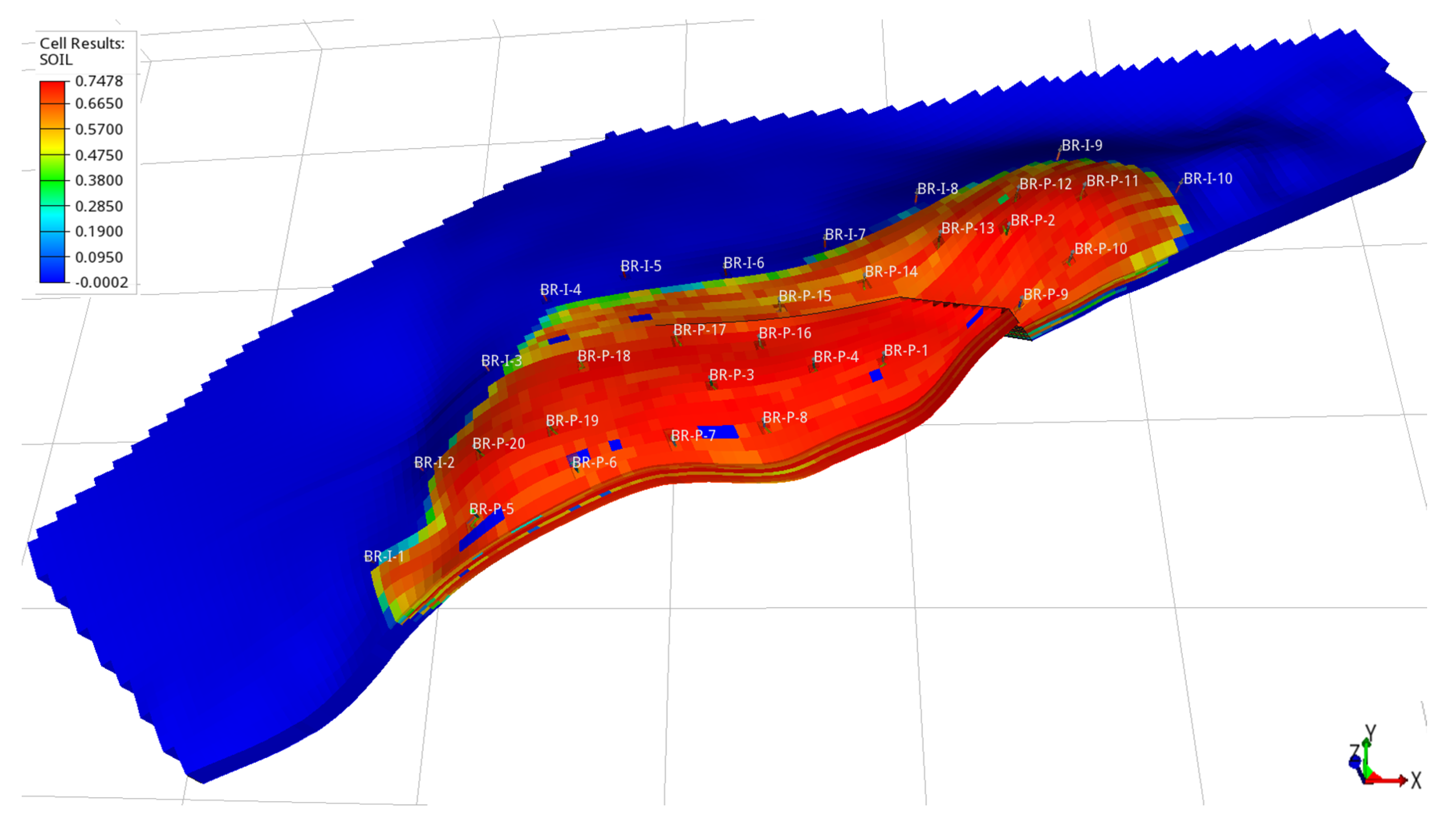
The dimensions of the reservoir model are 139 × 48 × 9, summing up to 60,048 gridblock, in which 44,550 are active. Figure 3 shows the location of the field wells, including 30 wells (20 inner producers and 10 injectors). The producers are located more centrally in the red area and labelled as BR-P-1-BR-P-20, while the injectors are located on the border and labelled as BR-I-1-BR-I-10, with water being the only injected fluid.

The initial ensemble of this benchmark contains 104 realizations of reservoir models, from which we take the first realization (#1) as our reference (true) case to generate the observed data. As for reservoir model variables, we consider porosity (PORO) and permeability along x-, y-, and z- directions (denoted by PERMX, PERMY, and PERMZ), summing up to 178,200 ($4 \times$ 44,550) uncertain petro-physical parameters to estimate in history matching.

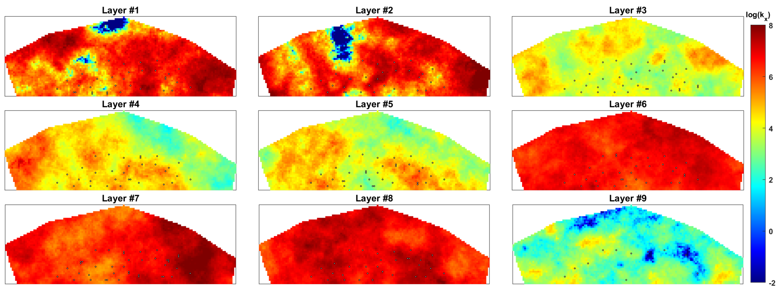
For illustration, Figure 4 and Figure 5 show the distributions of the porosity and the log permeability (along the x-direction), respectively, on each layer from realization number two ($\#2$) of the initial ensemble. As reported in [29], the permeability and porosity are linearly correlated, and the spatial distribution of the permeability is anisotropic, meaning that permeability distributions along different directions may not be the same.

In history matching, we condition reservoir models on three types of field data, namely, production, tracer, and 4D seismic data. The historical production data cover a period of 3647.5 days, with production forecasts from 3647.5 to 9869.5 days, where reservoir simulations are conducted using a black oil simulator (ECLIPSE©). The production data include well bottom hole pressure (WBHP), well oil and water rates (WOPR, and WWPR), summing up to 1400 data points. In addition, an injection of a water passive tracer pulse of 1.0 lb per STB is performed from day 749 to day 1812 in the injector well BR-I-6 (WTPCW06), summing up to 400 data points. To mimic the presence of measurement noise in real production data, here we also introduce certain zero-mean Gaussian white noise to the reference production and tracer data, for which the STD of the noise is set as 10% of the magnitude of each production or tracer data point, except for WBHP (for which the noise STD is set as 50 psi for each data point instead).

The 4D seismic data are obtained from three surveys: base (day 1), monitor #1 (day 991), and monitor #2 (day 2999). From each seismic survey, the seismic attributes (AVA data) are obtained using two different offset angles, near (10${}^{\circ }$) and mid (20${}^{\circ }$). The AVA data are in a seismic domain and do not possess physical locations in the reservoir coordinate system, meaning that the AVA data are in a different dimension compared to the dimension of the reservoir model. In this work, the dimension of the AVA data is 139 × 48 × 176 for each seismic survey, summing up to 7,045,632 data points in total [15]. We also introduce certain zero-mean Gaussian white noise to the AVA data, with the STD of the noise set to 30% of the magnitude as in [15].

In order to deal with the issue of big seismic data in history matching, and thereby the required memory, we choose to sparsely represent the AVA data by first applying 3D discrete wavelet transform (DWT) to the seismic data, and then (through a thresholding operation) selecting a small set of the resulted leading wavelet coefficients as the observations in history matching. For brevity, we skip the details of the DWT-based sparse data representation procedure. Readers are referred to [15,37] for more information.

From the algorithmic perspective, in the presence of the DWT-based sparse data representation procedure, the effective observation system with respect to 4D seismic data becomes

$$\mathcal{T}\left(\mathcal{W}\left({\mathbf{d}}^o\right)\right)=\mathcal{T}\left(\mathcal{W}\left({\mathbf{g}}^s\left({\mathbf{m}}_{\mathrm{true}}\right)\right)+\mathcal{W}\left(\delta \right)\right),$$

(21)

where $\mathcal{W}$ and $\mathcal{T}$ denote wavelet transformation and thresholding operators, respectively, and ${\mathbf{g}}^s$ corresponds to the seismic forward simulator, as discussed in Appendix A. By using the aforementioned formulation, we are able to represent the original 4D seismic (7,045,632 data points) by a much smaller set of 1896 wavelet coefficients, as elaborated in [15].

Experiment Settings

In our previous work [3], we have shown that adopting both production and tracer data in the Brugge benchmark helps improve the performance of history matching, in comparison to the choice of using production data only. The current work can be considered as a follow-up study, in which we aim to further examine the impacts of 4D seismic data on history matching, and show the complexity of the joint history matching problem in the presence of multiple types of field data. To this end, in the current work we conduct two experiments complementary to those in [3]:

• Case 1: using production and 4D seismic data;
• Case 2: using production, tracer, and 4D seismic data.

In both cases, we apply the DWT-based sparse data representation procedure to the seismic attributes obtained at three surveys for improved computational efficiency.

We use IES-RLM as the history matching algorithm, and equip it with the correlation-based adaptive localization scheme described in Section 2.2. We start the IES-RLM algorithm with ${\eta }^0=1$, with the reduction and increment factor being, 0.9 and 2, respectively. More specifically, if the average data mismatch is reduced at the current iteration step, then the $\eta$ value at the next iteration step is set to 0.9 times that at the current step; otherwise, the next $\eta$ value is set to 2 times the value of the current iteration step, and an inner loop is then activated to search for lower data mismatch.

To simultaneously history match multiple types of field data, we introduce a normalization procedure to adjust the relative weights assigned to different types of field data, as in [2]. Following the formulation in [3], we substitute the measurement error-covariance matrix ${\mathbf{C}}_{\mathrm{d}}$ in Equation (3) by the Schur product $diag\left(\mathbf{w}\right)\circ {\mathbf{C}}_{\mathrm{d}}$, where $\mathbf{w}$ is a vector to be specified later, and the operator $diag\left(\mathbf{w}\right)$ stands for a diagonal matrix whose diagonal elements are taken from the vector $\mathbf{w}$.

For production and tracer data, the elements of $\mathbf{w}$ are determined using the following rule:

$$w_k={\left(max(type\left({\mathbf{d}}_k^o\right))\times p(type\left({\mathbf{d}}_k^o\right))/{\sigma }_k\right)}^2,\mathrm{for}k=1,2,\cdots ,N_d,$$

(22)

where the operator $max(type\left({\mathbf{d}}_k^o\right))$ takes the maximum value of a given type of field data, and $type\left({\mathbf{d}}_k^o\right)$ stands for the type (WBHP, WOPR, WWPR or WTPCW06) of the k-th field-data point. Note that the value $max(type\left({\mathbf{d}}_k^o\right))$ is normalized by the measurement-noise STD ${\sigma }_k$ associated with the data point ${\mathbf{d}}_k^o$, aiming to mitigate potential problems caused by the different orders of magnitudes of the field data. The notation p represents a percentage value, which is set to $5\%$ if ${\mathbf{d}}_k^o$ is a type of production data (WBHP, WOPR, or WWPR), and to $20\%$ instead if ${\mathbf{d}}_k^o$ is a tracer data point (WTPCW06).

For seismic data, the elements of $\mathbf{w}$ are determined using the following rule:

$$w_k={\left(\left(\frac{median(abs(\hat{\mathcal{W}}({\mathbf{d}}_k^o)))}{0.6745}\right)/{\sigma }_k\right)}^2,$$

(23)

where $\widehat{\mathcal{W}}\left({\mathbf{d}}_k^o\right)$ is the wavelet coefficient belonging to the finest sub-band of $\mathcal{W}\left({\mathbf{d}}_k^o\right)$.

As aforementioned, 4D seismic data usually contain a large number of data points, which can dominate the updates during history matching. To overcome this noticed issue, a certain scaling factor s is introduced to adjust the relative weights assigned to production, tracer and 4D seismic data during history matching. The scaling factor is determined using data mismatch of the initial ensemble, which is computed using the following formula:

$${\mathrm{HM}}_j^i={(\Delta {\tilde{\mathbf{d}}}_j^i)}^T\Delta {\tilde{\mathbf{d}}}_j^i.$$

(24)

By using Equation (24), one can compute the scaling factor as follows:

$$s={\overline{HM}}_1^0/{\overline{HM}}_2^0,$$

(25)

where the overline denotes the mean value over the ensemble members, ${\overline{HM}}_1^0$ corresponds to the mean data mismatch value of 4D seismic data, and ${\overline{HM}}_2^0$ to that of production data (Case 1) or that of both production and tracer data (Case 2). Note that in Case 2, we group production and tracer data together to compute the mean of data mismatch. To construct the scaled observational data, one needs to multiply the observation data from group 2 by the scalar s, so that $\Delta {\tilde{\mathbf{d}}}_{j,2}^i$ is replaced by $[\Delta {\tilde{\mathbf{d}}}_{j,2}^i\times s]$.

To assess uncertainty reduction for each type of petro-physical parameter (PERMX, PERMY, PERMZ, and PORO) in the experiments, we use the Sum of Normalized Variance (SNV) [38], as in

$$\mathrm{SNV}=\sum _{k=1}^{N_{\mathrm{m}}}\frac{var(m_k^f)}{var(m_k^0)},$$

(26)

where $var(m_k^0)$ and $var(m_k^f)$ denote the variances of a particular type of petro-physical parameter distributed on the k-th active reservoir gridblock of the initial and final ensembles, respectively.

Finally, to assess and compare history matching performance, in terms of the discrepancy between an estimated reservoir model $\mathbf{m}$ and the true one ${\mathbf{m}}_{\mathrm{true}}$, we use the Root Mean Squared Error (RMSE), as in

$$\mathrm{RMSE}=\frac{\Vert \mathbf{m}-{\mathbf{m}}_{\mathrm{true}}{\Vert }_2}{\sqrt{N_{\mathrm{m}}}}.$$

(27)

4. Results and Discussions

This section focuses on illustrating the performance of the history matching of the two aforementioned experiments, in terms of data mismatch values during history matching (which is calculated through Equation (24)) and forecast periods, and also uncertainty quantification that is represented by mean, standard deviation, and RMSE of the final ensemble.

Table 1. Values of data mismatch and RMSE with respect to the initial ensemble, and the final ensembles of Cases 1 and 2.

	Initial Ensemble	Case 1	Case 2
Production data mismatch	$(7.7861\pm 4.5592)\times {10}^3$	$1.1586\times {10}^3\pm 1.4297\times {10}^2$$(-85.1196\%)$	$1.1400\times {10}^3\pm 1.1465\times {10}^2$$(-85.3585\%)$
Tracer data mismatch	$(3.9620\pm 2.6721)\times {10}^1$		$6.0112\pm 9.3504(-84.8279\%)$
4D Seismic data mismatch	$(9.2270\pm 3.4727)\times {10}^3$	$(6.3050\pm 1.6124)\times {10}^3$$(-31.6679\%)$	$(6.3960\pm 1.6680)\times {10}^3$$(-30.6817\%)$
RMSE (PERMX)	$1.5578\pm 0.5356$	$1.0284\pm 0.2160(-33.9838\%)$	$1.0540\pm 0.2332(-32.3405\%)$
RMSE (PERMY)	$1.5524\pm 0.5315$	$1.0686\pm 0.2280(-31.1646\%)$	$1.0522\pm 0.2286(-32.2211\%)$
RMSE (PERMZ)	$1.7523\pm 0.5454$	$1.2992\pm 0.2620(-25.8574\%)$	$1.2412\pm 0.2276(-29.1674\%)$
RMSE (PORO)	$0.0253\pm 0.0039$	$0.0240\pm 0.0034(-5.1383\%)$	$0.0242\pm 0.0035(-4.3478\%)$
RMSE (all parameters)	$1.4067\pm 0.4634$	$0.9866\pm 0.2011(-29.8642\%)$	$0.9700\pm 0.1961(-31.0443\%)$

summarizes the values of data mismatch ($mean\pm STD$) and RMSE ($mean\pm STD$) with respect to the initial ensemble and the final ensembles of the two experiments’ settings (Cases 1 and 2). In comparison with the initial ensemble, both experiments exhibit better history matching performance, in terms of both lower data mismatch and RMSE values. Comparing the results between the two different experiments shows that we achieve slightly lower data mismatch for production data (−0.2389%), but at the cost of a slightly higher data mismatch for 4D seismic data (+0.9862%), when jointly history matching production, tracer, and 4D seismic data (Case 2). In terms of RMSE, Case 2 contains lower average values for PERMY and PERMZ (−1.0565% and −3.3100%, respectively), but slightly higher ones for PERMX and PORO (+1.6433% and +0.7905%, respectively). In addition, the average RMSE values for all parameters together in Case 2 is slightly lower in comparison with Case 1, which indicates that the overall history matching performance in terms of RMSE tends to improve by adding more types of field data, but the complexity of the history matching process tends to increase. Note that in Case 2, only inter-well tracer from injector BR-I-6 was included in the history matching workflow, which provides additional information regarding well-to-well connectivity for the producers (BR-P-3, BR-P-4, BR-P-14, BR-P-15, BR-P-16, and BR-P-17), where tracer is detected. However, one cannot expect a substantial reduction in the overall data mismatch and RMSE values due to the use of the tracer data, as the inter-well tracer is usually detected in a limited number of production wells in the reservoir and tracer from a single injector well may not be sufficient to provide information to improve the connectivity of the entire reservoir. We discuss more about reservoir connectivity in the forecast analysis.

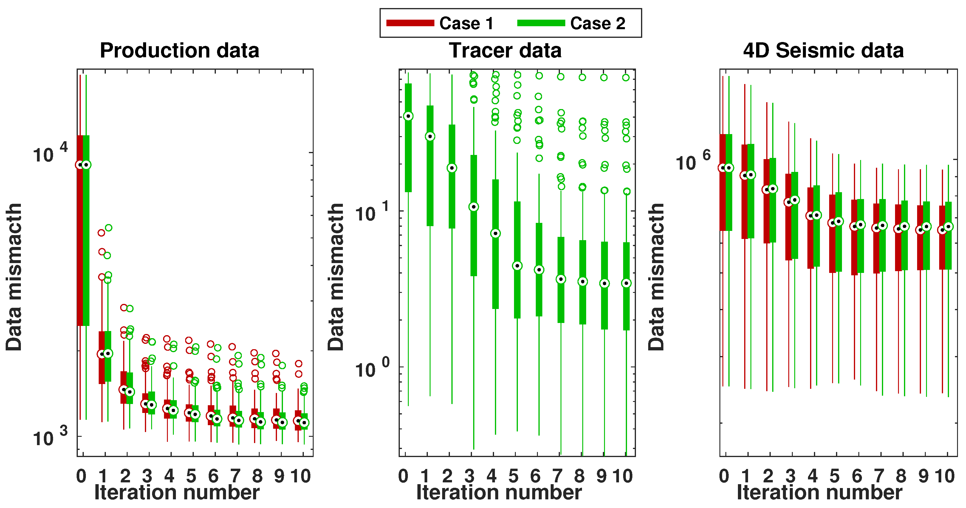
For illustration, Figure 6 reports the ensemble of data mismatch values obtained at each iteration step, in the form of box plots in Cases 1 and 2. In both cases, data mismatch values tend to decrease over the iteration steps for all types of field data. In addition, one can observe that main reductions of data mismatch values take place within the first few iteration steps for production data, and afterwards the changes of data mismatch values are less substantial. These main reductions in data mismatch are related to the changes of well bottom hole pressure (WBHP), which is strongly reduced in the first few iterations steps. Furthermore, the IES-RLM algorithm is close to convergence after 10 iterations steps, which is the maximum number of iterations used in the case studies.

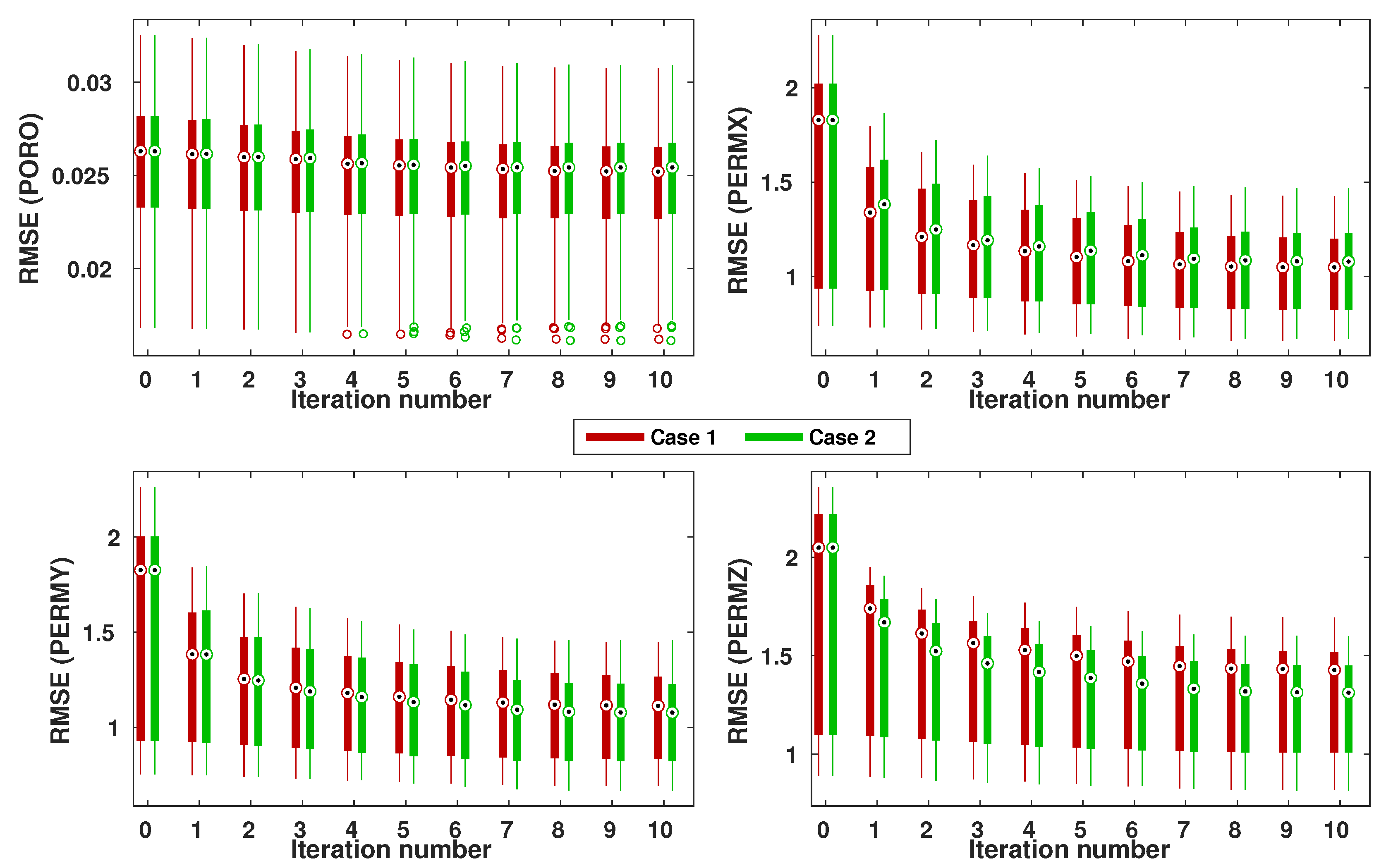
Similarly, Figure 7 shows box plots of RMSE values in the two case studies, for PERMX, PERMY, PERMZ and PORO, respectively. As one can see, the average RMSE values also tend to decrease over the iterations steps. Consistent with Table 1, the results show that jointly history matching production, tracer and 4D seismic data (Case 2) tends to result in lower mean RMSE values for PERMY and PERMZ, but slightly higher ones for PERMX and PORO, in comparison with the choice of history matching both production and 4D seismic data (Case 1).

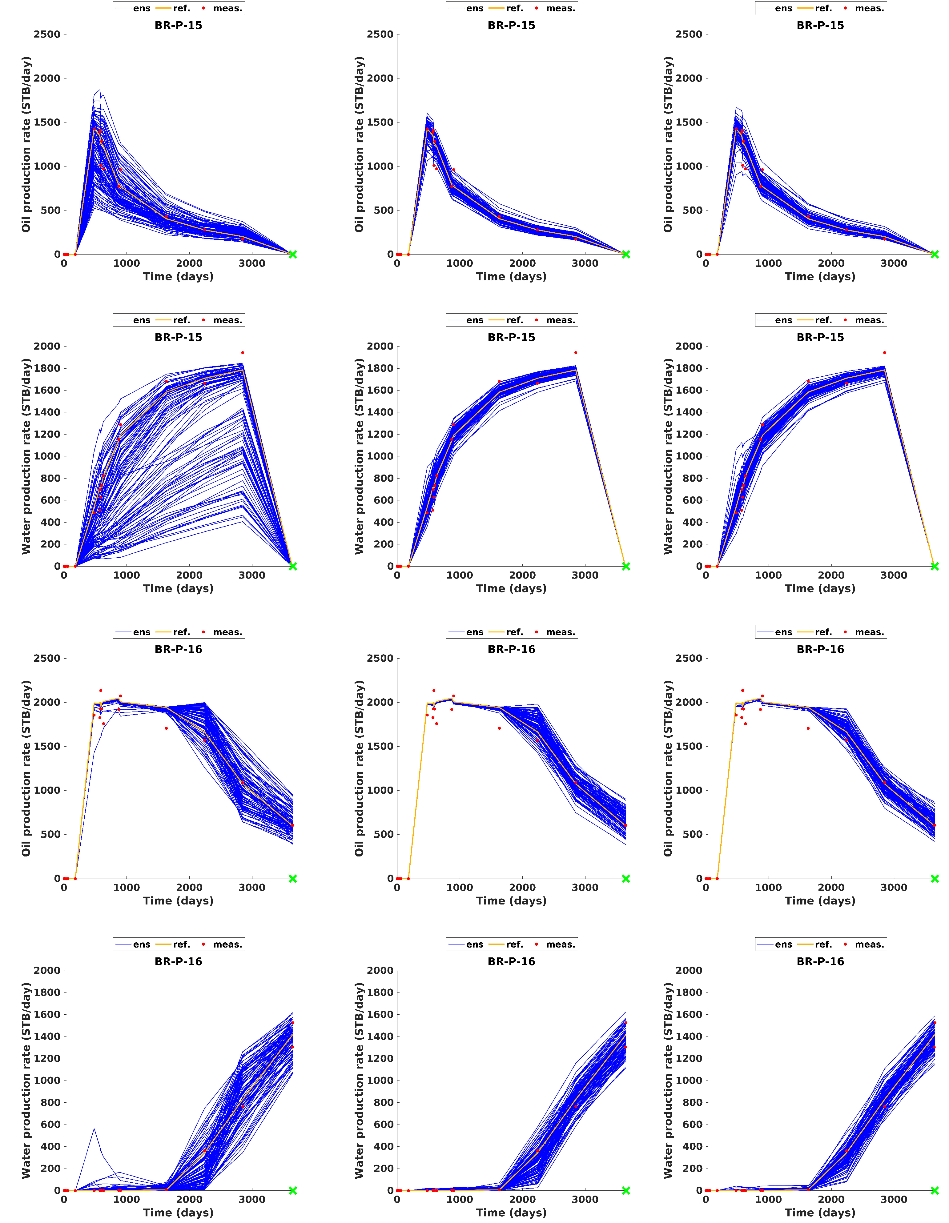
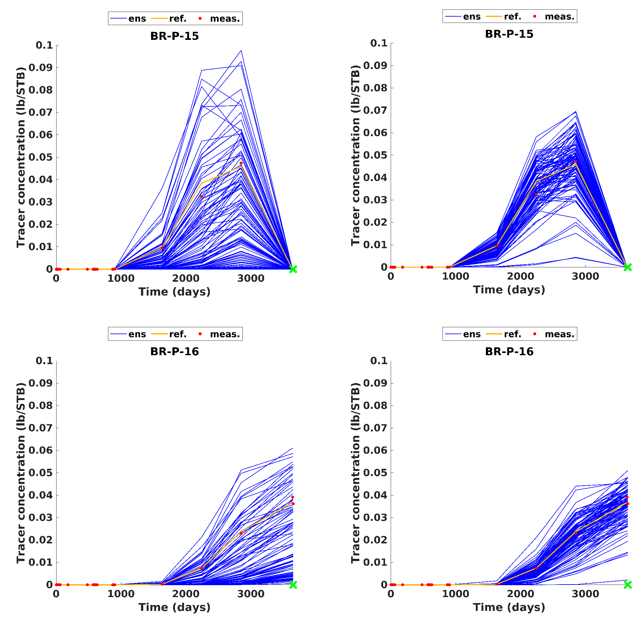
Figure 8 presents the profiles of WOPR and WWPR from well BR-P-15 and BR-P-16, with respect to the initial and final ensembles in the two case studies. In comparison to the initial ensemble, both cases indicate significant improvements in terms of reduced data mismatch and uncertainty (in terms of ensemble variability). For instance, compared to the choice of history-matching production and 4D seismic data (Case 1), one can see that the inclusion of tracer in Case 2 tends to slightly reduce the variability of the final ensemble of WWPR in BR-P-16, which means that the final ensemble follows the observed data better.

Similar to Figure 8, Figure 9 shows the profiles of tracer data injected in well BR-I-6 and recorded at wells BR-P-15 and BR-P-16, with respect to the initial and final ensembles in the two case studies. Here, the history matching performance is reasonably good in terms of data mismatch, e.g., for both production wells, history matching helps reduce data mismatch of the final ensembles, which is consistent with Table 1.

In addition,

Table 2. Parameter uncertainty reduction assessment in the different experiments.

Experiments	SNV (PORO)	SNV (PERMX)	SNV (PERMY)	SNV (PERMZ)
Case 1	$92.43\%$	$69.13\%$	$69.79\%$	$75.02\%$
Case 2	$92.94\%$	$69.27\%$	$69.28\%$	$71.93\%$

provides an assessment of parameter uncertainty reduction (in terms of SNV) in the two aforementioned experiments. As one can see, in both case studies, the final ensembles maintain substantial variability, meaning that the localization scheme is useful for preserving ensemble variability. Consistent with Table 1, Case 2 contains slightly lower SNV values for PERMY and PERMZ, while slightly higher ones for PORO and PERMX, in comparison with Case 1. As tracer data are more correlated to permeability, one may expect more uncertainty reduction for permeability than porosity. This is partially reflected by the results in Table 2, where there is a relatively stronger uncertainty reduction for PERMY and PERMZ (−0.51% and −3.09%, respectively).

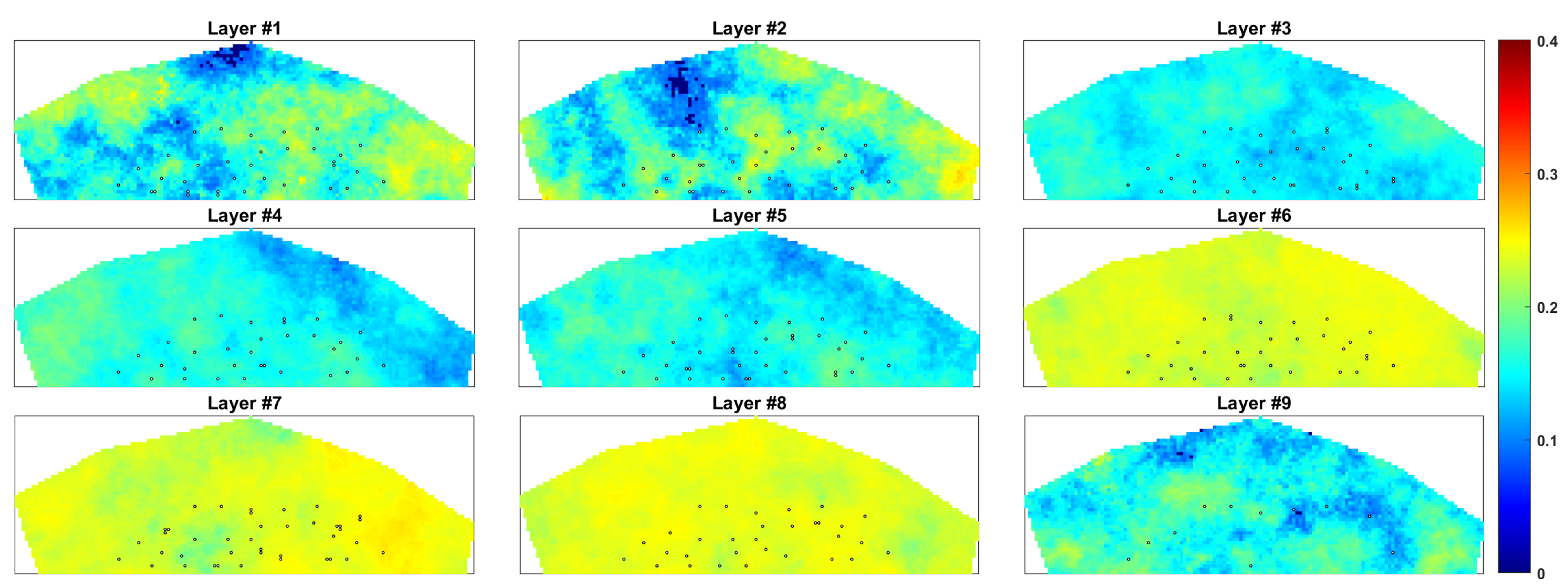
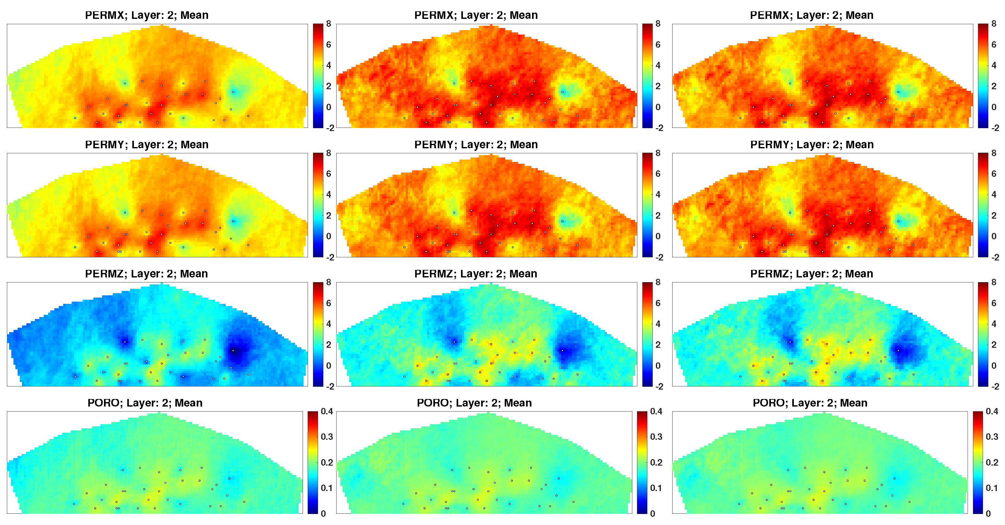
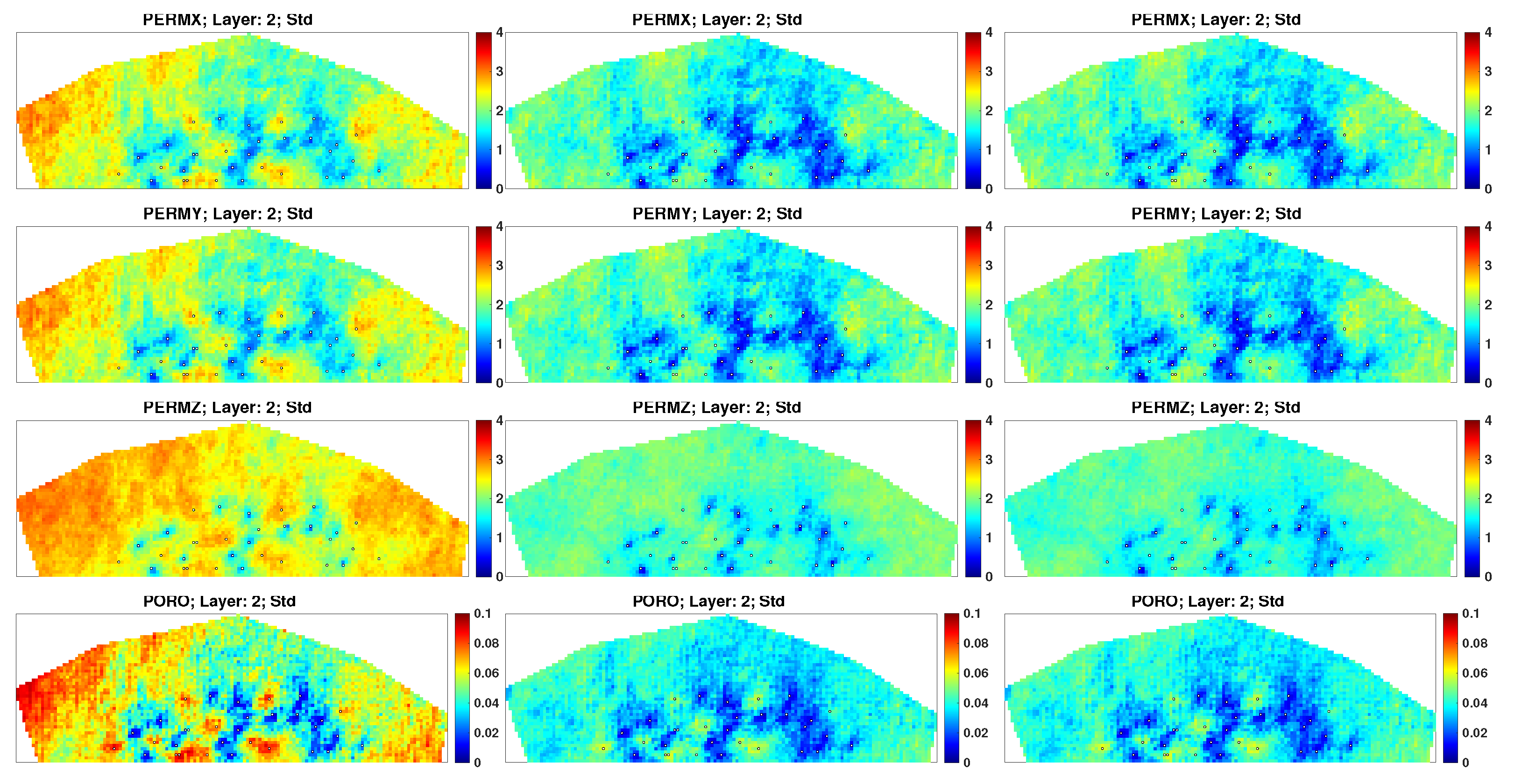
Another important aspect is to inspect the spatial distributions and standard deviations of the petro-physical parameters after history matching. Figure 10 and Figure 11 report mean and standard deviation maps of the petro-physical parameters on layer 2, with respect to the initial and final ensembles in Cases 1 and 2. After history matching, one can see that there are minor changes among different experiment results. Relative to the mean maps, our history matching workflow is able to capture the main aspects of the initial ensemble in both experiments. Meanwhile, the standard deviation maps of the two experiments indicate substantial variability after history matching, which means that the ensemble collapse is avoided.

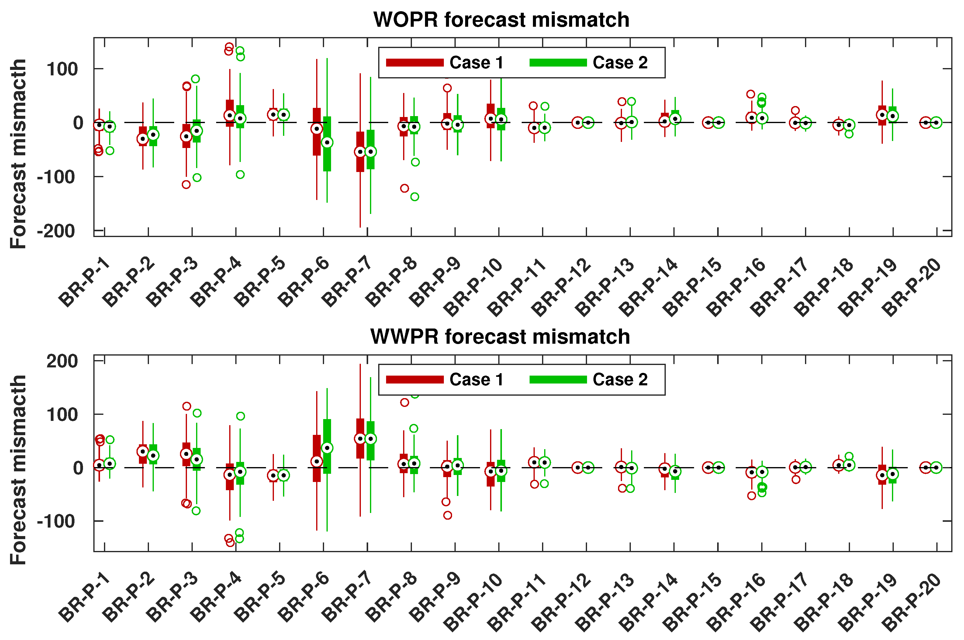
Finally, we forecast the production data beyond the history matching period using the final ensembles obtained in Cases 1 and 2. For comparison, we calculate the forecast data mismatch for WOPR and WWPR, which is the difference between simulated data of the reference model and an estimated ensemble of reservoir models at the forecast period, normalized by the STD of the WOPR and WWPR.

As aforementioned, we observed better history matching performance in terms of production data mismatch and RMSE values for PERMY and PERMZ parameters, when using production, tracer, and 4D seismic data (Case 2) during the history matching period. In terms of forecast mismatch, the comparison becomes a bit more complicated. As one can see in Figure 12, in some wells (e.g., BR-P-3, and BR-P-16), we observe lower forecast mismatch for the experiment in Case 2. However, in some other wells (e.g., BR-P-6), the situation is the opposite, and higher forecast mismatch is observed instead. The complexity of performance comparison may be partially due to the geological structure of the reservoir model. In this benchmark case, the presence of a fault could have a substantial influence on intra-well fluid flows, which means that it could be relatively easy for the tracer to flow to wells close to the fault and relatively difficult to more distant wells. By checking the distances between the injector–producer pairs, one can obtain a clue for a possible explanation for these noticed differences in the forecast performance. For instance, BR-P-6 is located close to the south-east boundary of the reservoir, so its communication to the other parts of the reservoir may appear weaker, since tracer data from BR-I-6 is not detected. Consequently, it could lead to lower correlations between production in BR-P-6 and the petro-physical parameters in a large part of the reservoir, which makes it more difficult to improve the qualities of estimated parameters close to BR-P-6, hence leading to higher forecast mismatch.

Other than the history matching performance, we also report in Appendix B the overall wall-clock time consumed in Cases 1 and 2. As one can see there, including seismic and/or tracer data into the history matching workflow substantially increases the computational time in our research environment. Nevertheless, the overall computational time is still at a reasonable and acceptable level, meaning that our proposed workflow has the potential for real field case studies.

5. Summary and Conclusions

In this work, we investigated a joint history matching problem with multiple types of field data and proposed a coherent way to integrate production, tracer, and 4D seismic data into a history matching workflow. The workflow is demonstrated in the Brugge benchmark case using the IES-RLM algorithm, with two different experiment settings (Cases 1 and 2).

The main idea behind adding multiple types of field data is to improve the reliability of reservoir models and consequently, the forecast performance. Through two different experiments, it is shown that jointly history matching production, tracer, and 4D seismic data results in lower data mismatch for production data and lower RMSE for PERMY and PERMZ, but at the cost of slightly higher data mismatch for 4D seismic data and RMSE for PORO and PERMX. In terms of the averaged RMSE over all estimated petro-physical parameters, the reliability of the reservoir models is improved in Case 2 in comparison with Case 1.

In both cases, adopting correlation-based adaptive localization helps to maintain substantial ensemble variability even in the presence of multiple types of field data, and ensemble collapse of reservoir models is avoided. Also shown in [3], the localization scheme appears beneficial to achieve a better performance during the forecast period. By a well-to-well analysis of the data mismatch during the forecast period, it is observed that both experiments appear to have good data mismatch. Nevertheless, inter-well tracer data seem to be helpful for further reducing data mismatch, which indicates a better inter-well communication in the reservoir.

Although a better history matching performance (in terms of RMSE) is achieved with the inclusion of tracer data in Case 2, the complexity of the history matching process is increased by adding more types of field data. In the proposed workflow, we adopted a scaling procedure to adjust the relative weights among production, tracer, and 4D seismic data, which appears to work reasonably well. However, to further improve the history matching performance, it could be beneficial to develop more sophisticated methods to better balance the influence of multiple types of field data in ensemble-based history matching. Other possible lines of future research would be to consider the use of multiple tracer injectors at different reservoir locations, and to extend our proposed workflow to hydraulically or naturally fractured reservoirs [39,40]. Such investigations will be considered in our future work.