Drunkard Adaptive Walking Chaos Wolf Pack Algorithm in Parameter Identification of Photovoltaic Module Model

Abstract

The rapid and accurate identification of photovoltaic (PV) model parameters is of great significance in solving practical engineering problems such as PV power prediction, maximum power point tracking and battery failure model recognition. Aiming at the shortcomings of low accuracy and poor reliability and being easy to fall into local optimization when standard intelligent optimization algorithms identify PV model parameters, a novel drunken adaptive walking chaotic wolf swarm algorithm is proposed, which is named DCWPA for short. The DCWPA uses the chaotic map sequence to initialize the population, thus to improve the diversity of the initial population. It adopts the walking direction mechanism based on the drunk walking model and the adaptive walking step size to increase the randomness of walking, enhance the individual’s ability to explore and develop and improve the ability of algorithm optimization. It also designs the judgment conditions for half siege in order to accelerate the convergence of the algorithm and improve the speed of the algorithm. In the iterative process, according to the change of the optimal solution, the Hamming Distance is used to judge the similarity of individuals in the population, and the individuals in the population are constantly updated to avoid the algorithm from stopping evolution prematurely due to falling into local optimization. This paper firstly analyzes the time complexity of the algorithm, and then selects eight standard test functions (Benchmark) with different characteristics to verify the performance of the DCWPA algorithm for continuous optimization, and finally the improved algorithm is applied for parameter identification of PV models. The experiments show that the DCWPA has higher identification accuracy than other algorithms, and the results are more consistent with the measured data. Thus, the effectiveness and superiority of the improved algorithm in identifying solar cell parameters are verified, and the identification effect of the improved algorithm on solar cell parameters under different illumination is shown. This research provides a new idea and method for parameter identification of a PV module model.

1. Introduction

Solar energy is characterized as non-polluting, renewable, cheap and easy to obtain, thus considered to be an effective solution for energy shortage and environmental pollution caused by industrial and economic development [1]. A photovoltaic (PV) system is a collection device of solar energy that converts solar energy into electrical energy, which has attracted great attention from scholars. 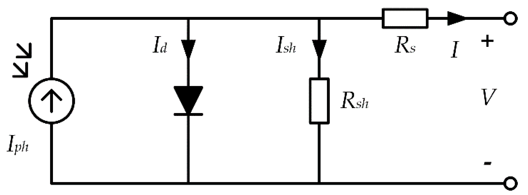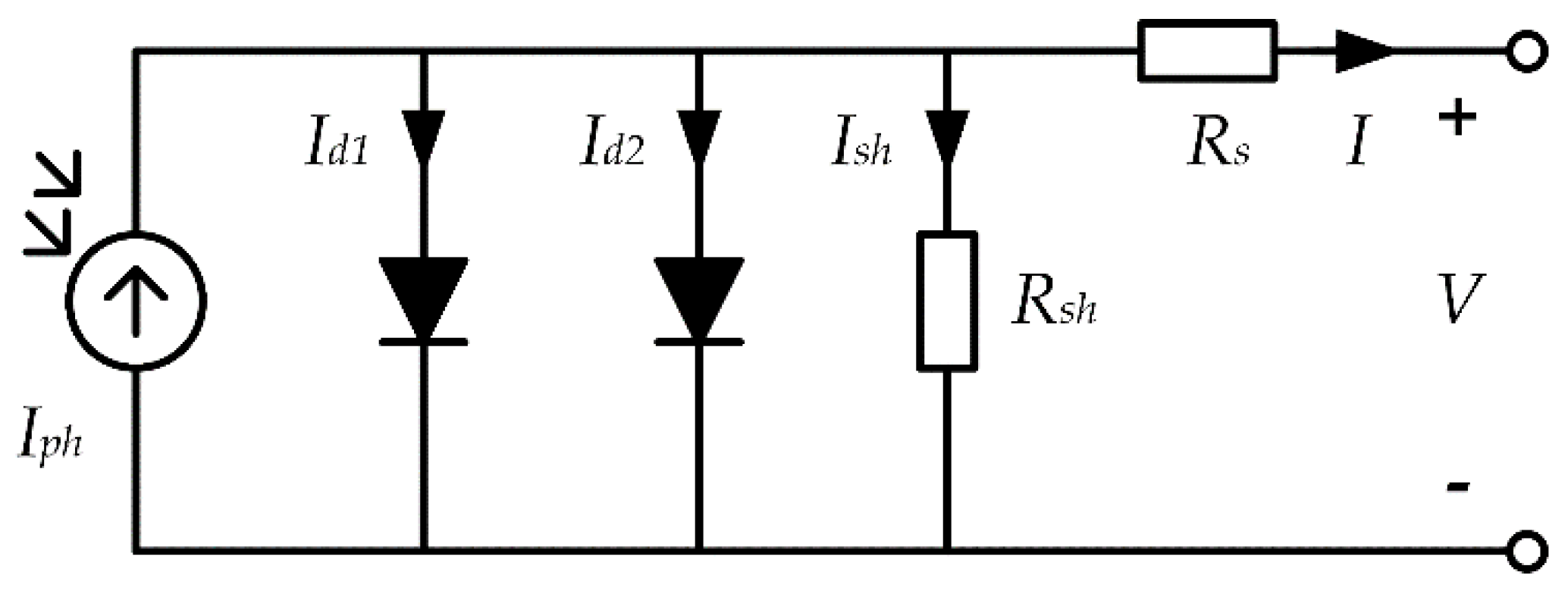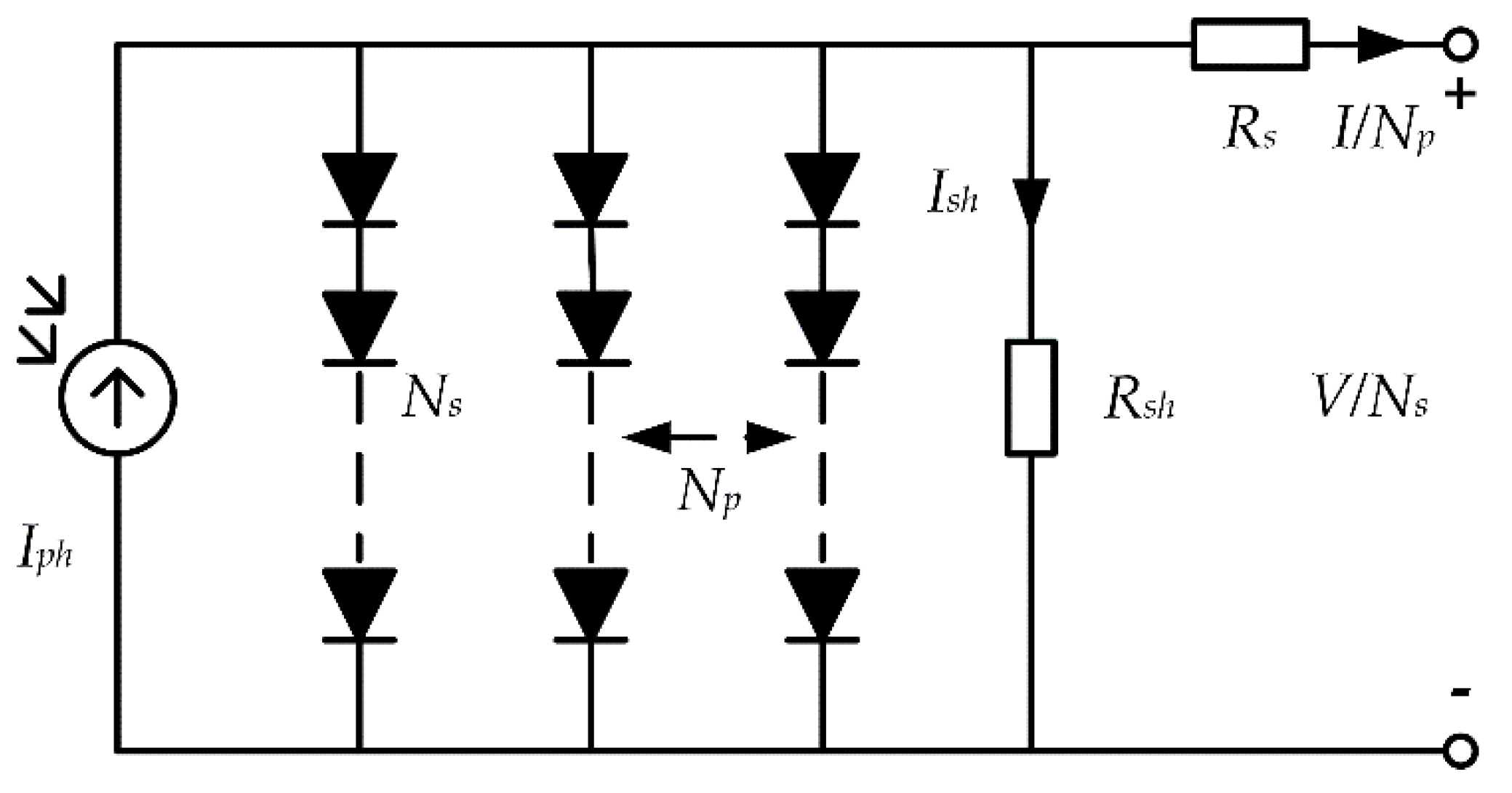In order to better design and apply fault diagnosis [2] and maximum power-point-tracking control [3] and other technologies of a PV system, it is very important to establish a mathematical model that can describe the current–voltage relationship in PV systems with high accuracy. In recent years, scholars at home and abroad have conducted a lot of research on the output characteristic models of PV system. The most commonly seen ones are the single-diode model (SDM) [4], the double-diode model (DDM) and the PV module model [5,6]. The accuracy of a PV model mainly depends on its model parameters, whose availability usually decreases due to aging, faults and unstable operating conditions. Therefore, accurate, stable and efficient identification of these PV model parameters is crucial for the evaluation, optimization and control of PV models. Parameter identification for a PV system model can be regarded as a function optimization problem, but because its search space is nonlinear and multi-modal, it is easy to fall into local optimum in the solution, which puts forward higher requirements for the solution [7].

The characteristics of swarm intelligence are clearly manifested in the behavior of organisms that adjust themselves according to the perceived information. Swarm intelligence is the information interaction between biological individuals, groups and environments that follow simple rules, and the characteristics of intelligence emerge as a whole. With the deepening of relevant research on Swarm Intelligence (SI), particle swarm optimization (PSO) [8], artificial fish swarm algorithm (AFSA) [9], ant colony algorithm [10], bacterial colony algorithm [11], artificial bee colony algorithm (ABC) [12], wolf pack algorithm [13] and their corresponding improved algorithms [14,15,16] have been proposed successively. Simple, robust, adaptable and applicable to wide ranges, these algorithms are effective ways to solve all kinds of complex optimization problems and have also been widely used for model parameter identification of a PV system [17,18,19,20,21,22,23,24,25]. Ref. [22] proposes a particle swarm algorithm (Classified Perturbation Mutation based Particle Swarm Optimization, CPMPSO) to seek solution for perturbation variation classification of PV system model parameter identification. It uses the damping constraint processing strategy to avoid falling into local optimization. Ref. [23] proposes a Logistic Chaotic Java to solve the parameter identification problem. The Logistic chaotic mapping strategy is introduced in the update stage of the algorithm to improve the population diversity. At the same time, the chaotic mutation strategy is introduced in the search stage to balance the search and exploration ability of the algorithm, but it also turns out to be easy to fall into local optimization in the later stage of the algorithm. Ref. [24] introduces the multiple learning backtracking search algorithm (MLBSA) for parameter identification of different PV models. Xu Yan et al. [25] propose a PV model parameter identification method based on a hybrid leapfrog algorithm. The update strategy of this method is directional and has strong local search ability, which can effectively solve the problem that the algorithm is easy to fall into local optimum. However, the solution steps of the algorithm are relatively complex, and the solution time is long. The intelligent optimization algorithm and its improved algorithm can globally optimize the parameters of a PV model on the basis of a small amount of experimental data, achieving satisfactory results with high precision and small errors, which can effectively meet the actual needs of some projects. However, due to the limitations of the algorithm’s own optimization mechanism, it is difficult for most algorithms to find the exact global optimal solution in practice. Therefore, it is still a challenge to design a highly competitive intelligent optimization algorithm to identify the parameters of a PV system model.

Wolf pack is a type of biological population with strong cognitive ability and rigorous social organization structure. Confronted with the “survival of the fittest” rule in a harsh environment, they have formed extremely sophisticated and efficient group intelligence behaviors such as cooperative hunting, enemy defense, reproduction, child rearing, etc. They have clear social class and labor division, and the group has demonstrated high intelligence features. Therefore, Yang et al. [26] propose a wolf swarm search algorithm based on the hunting behavior of wolves, which provides a better idea for solving complex problems. In 2013, Wu Husheng et al. [13] deeply analyzed the roles and behaviors of wolves in wolf pack hunting and designed a new wolf pack algorithm (WPA) based on the two rules of “winner as the king” and “survival of the strong” and the three behaviors of “walk, summon and siege”. The algorithm has good performance in global search and local exploration and shows great advantages in solving efficiency. It has been widely used in solving many practical problems such as 0–1 knapsack problem [27], TSP problem [28] and the path optimization problem [29]. Moreover, many scholars have improved the WPA in practical application in terms of too many parameters, high consumption of computing resources, long computing time and being easy to fall into local optimization, etc., and put forward a large number of improved algorithms [30,31,32,33,34]. Although a large number of improved algorithms have been proposed, the WPA is still rarely used for solving practical complex engineering problems, such as parameter identification of a PV model, and its efficiency and accuracy for solving complex optimization problems need to be further improved.

Aiming to avoid the low accuracy of the current intelligent optimization algorithm and the nonlinear and complexity of a PV module model, this paper proposes an improved Wolf Pack Algorithm (WPA) for parameter identification of a PV model based on the analysis of the basic Wolf pack algorithms. This algorithm uses the chaotic map sequence to initialize the population, thus to improve the diversity of the initial population. It adopts the walking direction mechanism based on the drunk walking model and the adaptive walking step size to increase the randomness of walking, enhance the individual’s ability to explore and develop and improve the ability of algorithm optimization. It also designs the judgment conditions for half siege in order to accelerate the convergence of the algorithm and improve the speed of the algorithm. In the iterative process, according to the change of the optimal solution, the Hamming Distance is used to judge the similarity of individuals in the population, and the individuals of the population are constantly updated to avoid the algorithm from stopping evolution prematurely due to falling into local optimization. This paper firstly analyzes the time complexity of the algorithm and then selects eight standard test functions (Benchmark) with different characteristics to verify the performance of the DCWPA algorithm for continuous optimization, and finally the improved algorithm is applied to the parameter identification problem of PV models. The experimental results show that the DCWPA has higher identification accuracy than other algorithms, and the results are more consistent with the measured data. Thus, the effectiveness and superiority of the improved algorithm in identifying solar cell parameters are verified, and the identification effect of the improved algorithm on solar cell parameters under different illumination is shown.

This paper is organized as follows. Section 2 introduces the PV module parameter identification problem and its mathematical model. Section 3 introduces the basic wolf pack algorithm and carefully analyzes its performance and its shortcomings. Section 4 proposes a specific improvement strategy for the problems existing in the basic wolf pack algorithm, forming the DCWPA. In Section 5, benchmark functions are used to verify the performance of the DCWPA for solving continuous optimization problems. In Section 6, experiments are conducted to evaluate the effectiveness and superiority of the proposed algorithm for solving the parameter identification problem of PV models. In Section 7, the conclusion is drawn for the future work.

2. Mathematical Model of PV System Module

2.1. Problem Description

At present, the single-diode and double-diode models are the most widely used. On the basis of these two models, the PV module model has also been further developed.

2.1.1. Single-Diode Model

Single-diode model (SDM) has the advantages of simplicity and accuracy. It is often widely used to describe the static characteristics of PV systems. The equivalent circuit diagram of the model is shown in Figure 1.

The model consists of a current source connected in parallel to the diode, a shunt resistance representing the leakage current and a series resistance representing the load current related loss. The output current $I$ is shown in Equation (1).

$$\{\begin{array}{c}I=I_{ph}-I_d-I_{sh}\\ I_d=I_o·\left[\exp (\frac{q·\left(V+I·R_s\right)}{a·k·T})-1\right]\\ I_{sh}=\frac{V+I·R_s}{R_{sh}}\end{array}$$

(1)

Here, $I_{ph}$ is photogenerated current, $I_d$ is diode current, $I_{sh}$ is the current of parallel resistor, $I_o$ is diode reverse saturation current, $a$ is the ideal factor of diode, $R_s$ and $R_{sh}$ represent series and parallel resistance, respectively, and $V$ is the battery output voltage, $k$ refers to the Boltzmann constant ($k=1.3806503\times {10}^{-23} \mathrm{J}/\mathrm{K}$), $q$ represents electron charge ($q=1.60217646\times {10}^{-19} \mathrm{C}$), and $T$ is the junction temperature expressed in Kelvin temperature. Among them, five unknown parameters ($I_{ph}$, $I_o$, $R_s$, $R_{sh}$, $a$) need to be extracted in SDM.

2.1.2. Double-Diode Model

Compared with SDM, the double-diode model (DDM) considering the influence of compound current loss in the depletion region is more accurate. Therefore, DDM is also commonly used in the modeling of PV cells [35]. The model has two diodes in parallel with the current source and a shunt resistance for shunting the photogenerated current source. One is used as a rectifier, and the other is used to simulate charge recombination current. The equivalent circuit of the dual diode model is shown in Figure 2.

The output current $I$ of DDM can be calculated by Equation (2).

$$\{\begin{array}{c}I=I_{ph}-I_{d1}-I_{d2}-I_{sh}\\ I_{d1}=I_{o1}·\left[\exp (\frac{q·\left(V+I·R_s\right)}{a_1·k·T_t})-1\right]\\ I_{d2}=I_{o2}·\left[\exp (\frac{q·\left(V+I·R_s\right)}{a_2·k·T})-1\right]\\ I_{sh}=\frac{V+I·R_s}{R_{sh}}\end{array}$$

(2)

Here, $I_{d1}$ and $I_{d2}$ represent the current of two diodes, respectively, $I_{o1}$ and $I_{o2}$ are diffusion current and saturation current, respectively, and $a_1$ and $a_2$ refer to the ideal factors of the two diodes. DDM needs to extract seven unknown parameters, namely $I_{ph}$, $I_{o1}$, $I_{o2}$, $R_s$, $R_{sh}$, $a_1$ and $a_2$.

2.1.3. PV Module Model

The PV module is composed of several solar cell units in series and parallel, and its equivalent circuit is shown in Figure 3.

For a single-diode PV module, the relationship between current and voltage is as follows.

$$I=I_{ph}·N_p-I_o·N_p\left[\exp (\frac{q·\left(V+I·R_s·N_s/N_p\right)}{a·N_s·k·T})-1\right]-\frac{V+I·R_s·N_s/N_p}{R_{sh}·N_s/N_p}$$

(3)

where $N_s$ and $N_p$ are the number of solar cells in series or in parallel, respectively. The PV module model needs to extract five unknown parameters, namely $I_{ph}$, $I_o$, $R_s$, $R_{sh}$ and $a$.

2.2. Objective Function

The main purpose of parameter identification of a PV model is to find the optimal value of unknown parameters and minimize the difference between measured data and calculated current data. The problem is usually transformed to an optimization problem and reached by an optimization algorithm. Therefore, the error function of each pair of measured and calculated current data points of each model is given in

Table 1. Error functions of the three models.

No.	Type	Model
1	Single-diode model	$\{\begin{array}{c}f\left(V,I,x\right)=I_{ph}-I_o·\left[\exp (\frac{q·\left(V+I·R_s\right)}{a·k·T})-1\right]-\frac{V+I·R_s}{R_{sh}}-I\\ x=\left[I_{ph},I_o,R_s,R_{sh},a\right]\end{array}$
2	Double-diode model	$\{\begin{array}{c}f\left(V,I,x\right)=I_{ph}-I_{o1}·\left[\exp (\frac{q·\left(V+I·R_s\right)}{a_1·k·T})-1\right]-I_{o2}·\left[\exp (\frac{q·\left(V+I·R_s\right)}{a_2·k·T})-1\right]-\frac{V+I·R_s}{R_{sh}}-I\\ x=\left[I_{ph},I_{o1},I_{o1},R_s,R_{sh},a_1,a_2\right]\end{array}$
3	PV module based the SDM	$\{\begin{array}{c}f\left(V,I,x\right)=I_{ph}·N_p-I_o·N_p\left[\exp (\frac{q·\left(V+I·R_s·N_s/N_p\right)}{a·N_s·k·T})-1\right]-\frac{V+I·R_s·N_s/N_p}{R_{sh}·N_s/N_p}-I\\ x=\left[I_{ph},I_o,R_s,R_{sh},a,N_p,N_s\right]\end{array}$

. In order to quantify the overall difference, the root mean square error (RMSE) in Equation (4) is taken as the objective function. Here, the problem of parameter identification of a PV model is transformed into the problem of finding the minimum value of the objective function.

$$RMSE\left(x\right)=\sqrt{\frac{1}{N}{\displaystyle \sum }_{k=1}^{N}f{(V_k,I_k,x)}^2}$$

(4)

3. Basic Wolf Pack Algorithm

3.1. Basic Principles

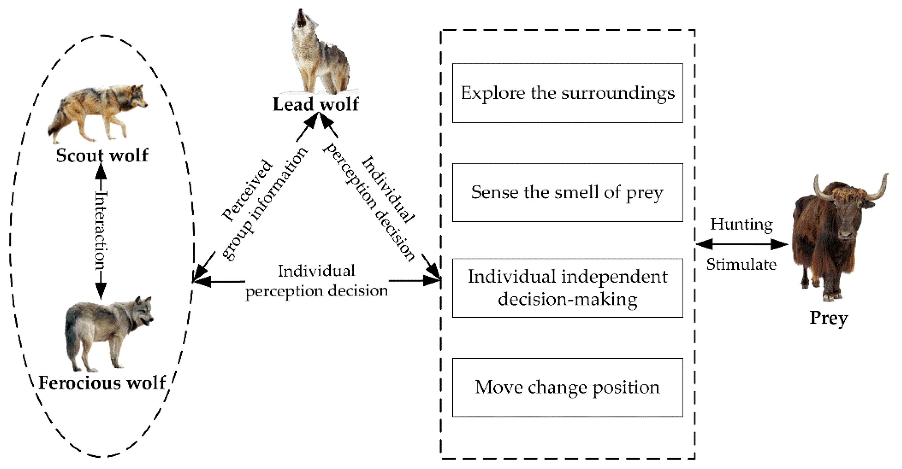
In nature, wolves have a strict social division mechanism and efficient cooperative hunting mode. Usually, there are three kinds of wolves in the wolf pack: the lead wolf, the scout wolf and the fierce wolf. The lead wolf makes overall planning, the scout wolf roams and searches, and the fierce wolf rounds up and attacks. The division of labor is clear, and each performs its own duties. After catching prey, it is distributed according to work and the survival of the fittest so that the population capacity continues to evolve [13]. Therefore, three intelligent behaviors (wandering behavior, summoning behavior and siege behavior) and two basic mechanisms (the selection mechanism of winner as the lead wolf and the evolution mechanism of survival of the fittest) can be abstracted from the swarm intelligence model of wolves [13]. On this basis, the WPA is proposed, and its basic principle model is shown in Figure 4.

3.2. Basic Process

Consider the area where wolves hunt as a $N\times D$ Euclidean space where the size of wolf pack is $N$ and the dimension of the space is $D$. The position of wolf $i$ is $X_i=\left(x_{i1},x_{i2},\dots ,x_{iD}\right)$, where $x_{id}$ is the position of wolf $i$ in the $d^{th}\left(d=1,2,\dots ,D\right)$ dimension space. The concentration of the prey smell perceived by wolf $i$ (that is, the fitness value of the objective function) is recorded as $Y_i$, then $Y_i=f\left(X_i\right)\left(i=1,2,\dots ,N\right)$. Taking solving the maximum fitness value of the function as an example, the following two basic mechanisms and three intelligent behaviors in the wolf pack algorithm are explained.

1.

Selection mechanism of the lead wolf. In the process of wolf rounding up, the lead wolf is constantly changing according to the principle of “winner as the king”. In the initial wolf pack, the individual wolf with the largest objective function value is selected as the lead wolf. During the round-up process, if there is an individual wolf that is superior to the target function value corresponding to the position of the lead wolf, the individual wolf will immediately replace the original lead wolf. In the whole process, the position of the lead wolf is denoted as $g$, and its corresponding objective function value is denoted as $Y_{lead}$.

2.

Evolution mechanism of the wolf pack. The food distribution rules of the wolf pack reward on merit will inevitably lead to the starvation of some individual wolves with weak ability. Therefore, in the wolf pack algorithm, $R$ individual wolves with the worst objective function value are removed, and $R$ individual wolves are randomly produced to update the wolf pack, where $R\in \left[N/\left(2\beta \right),N/\beta \right]$ and $\beta$ is the proportion factor of population renewal.

3.

Wandering behavior. The scout wolf advances one step in $h$ directions, respectively, calculates the fitness value of the positions after moving forward and then returns to the original position. After one step in the $p^{th}$ direction, the position of the scout wolf $i$ in the $d^{th}$ dimensional space is shown in Equation (5). In the $h$ directions, the scout wolf advances in the direction with the largest fitness value and greater than the current position fitness value $Y_i$. We continue to perform the above walking behavior and stop until the walking reaches the maximum number of steps $T_{max}$ or when $Y_i>Y_{lead}$ occurs, which determines the updated lead wolf.

$$x_{id}^p=x_{id}+ste{p}_a^d\times \sin \left(2\pi \times \frac{p}{h}\right)$$

(5)

Here $ste{p}_a^d$ is the walking step and $d=1,2,\dots ,D$; $P=1,2,\dots ,h$, because the search ability of each scout wolf is different, the value of $h$ is also different, which takes a random integer. Generally, the larger $h$ is, the more detailed the scout wolf search is, but the slower the algorithm calculation speed is.

4.

Summoning behavior. After the wandering behavior is over, the lead wolf calls all wolves to approach him. After receiving the call information of the lead wolf, fierce wolf $i$ quickly approaches the lead wolf with a large attack step $ste{p}_b^d$ according to Equation (6). If fierce wolf $i$ finds a position with a greater fitness value than the current position of the lead wolf on the way to the lead wolf, fierce wolf $i$ will replace the lead wolf and call; otherwise, the fierce wolf $i$ continues to perform the summoning behavior until the siege conditions are met: $L_{ig}^k\le L_{near}$.

$$x_{id}^{k+1}=x_{id}^k+ste{p}_b^d\times \frac{\left(g_d^k-x_{id}^k\right)}{\left|g_d^k-x_{id}^k\right|}$$

(6)

$L_{near}$ is the judgment distance turning into siege behavior, and $L_{near}$ can be calculated by Equation (7).

$$L_{near}=\frac{1}{D·\omega }·{\displaystyle \sum }_{d=1}^D\left|{\max }_d-{\min }_d\right|$$

(7)

${\max }_d$ and ${\min }_d$ are the upper and lower bounds of the value of the variable $x$ in the $d^{th}$ dimensional space, respectively.

Suppose the distance between the fierce wolf $i$ and the lead wolf in the $k^{th}$ generation is $L_{ig}^k$, as shown in Equation (8), $L_{ig}^k$ can be calculated by using the Manhattan distance.

$$L_{ig}^k={\displaystyle \sum }_{d=1}^D\left|x_{id}^k-g_d^k\right|$$

(8)

In the above equation, $x_{id}^k$ represents the position of the fierce wolf $i$ in the $d^{th}$ dimensional space in generation $k$, $g_d^k$ represents the position of the lead wolf in the $d^{th}$ dimensional space in generation $k$, and $x_{id}^{k+1}$ represents the position of the fierce wolf $i$ in the $d^{th}$ dimensional space in generation $k+1$.

5.

Siege behavior. Take the position of the lead wolf as the position of the prey, and all wolves siege the prey according to Equation (9). During the siege, if a new prey is found and its corresponding fitness value is greater than the current prey fitness value, update the prey location and siege the new prey until the prey is captured.

$$x_{id}^{k+1}=x_{id}^k+\lambda \times ste{p}_c^d\times \left|g_d^k-x_{id}^k\right|$$

(9)

where $\lambda$ takes the random number within (0,1), and $ste{p}_c^d$ represents the siege step length.

There are three steps in the WPA: walking step length $ste{p}_a^d$, running step length $ste{p}_b^d$ and siege step length $ste{p}_c^d$. The relationship of the three steps is shown in Equation (10):

$$ste{p}_a^d=ste{p}_b^d/2=2·ste{p}_c^d=\frac{\left|{\max }_d-{\min }_d\right|}{S}$$

(10)

In the above formula, $S$ represents the step size factor. The larger $S$ is, the more detailed the search is.

3.3. Performance Analysis

In the WPA, the walk behavior makes the algorithm have better traversality, so the algorithm has strong global exploration ability. The lead wolf selection mechanism and calling behavior make the wolves gather quickly and accelerate the convergence speed of the algorithm. Moreover, during the siege, the wolves further refine the search near the current optimal solution, which improves the local exploration ability of the algorithm. In addition, the renewal mechanism of wolves not only maintains the population advantage, but also helps to jump out of the local optimum. Therefore, the WPA shows better optimization performance. However, the algorithm still shows some shortcomings in practical application, as follows:

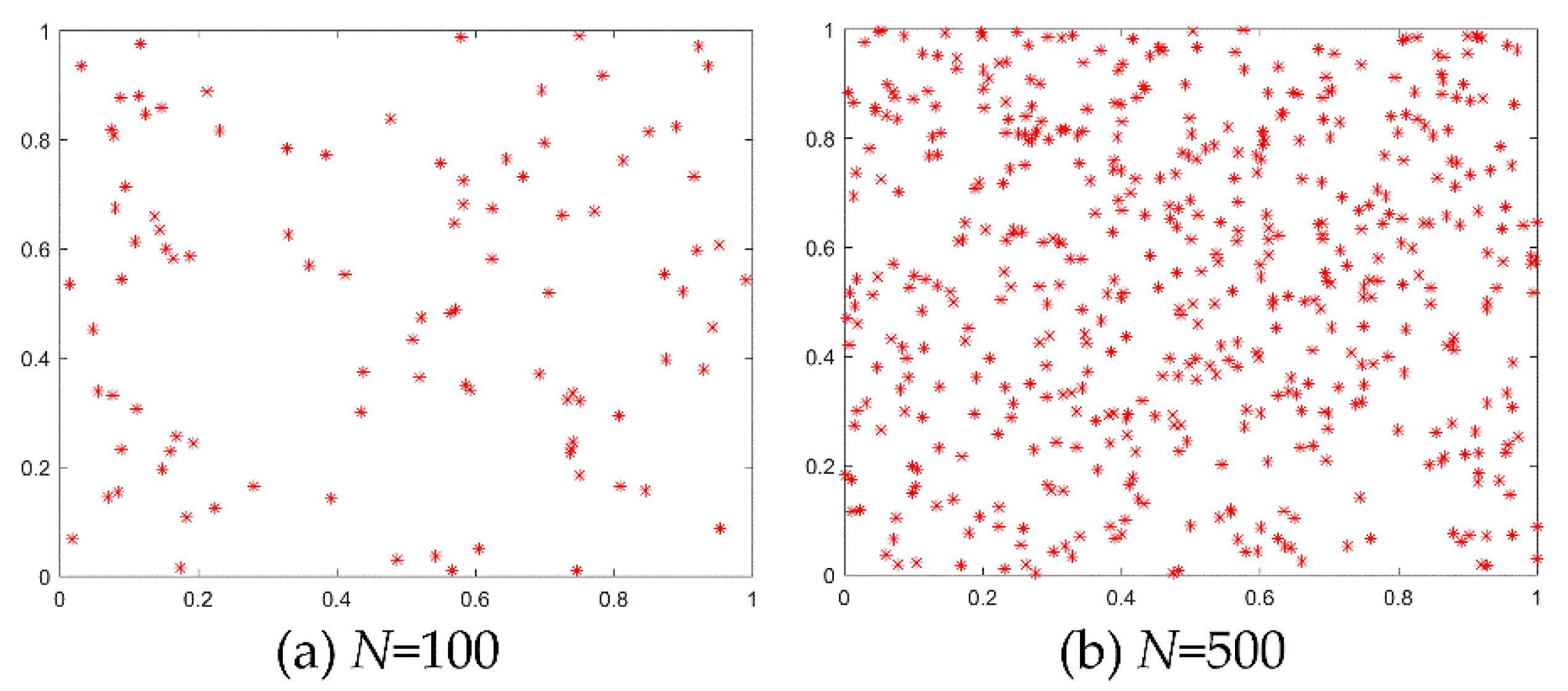
Disadvantage 1: The population initialization of the WPA generally adopts the way of pseudo-random number, so the population cannot cover the solution space evenly. If we invoke all the rand function in MATLAB software to initialize the two populations of size 100 and 500, respectively, as shown in Figure 5, the individuals in the initial population overlap each other, and some areas are blank. As a result, the initial population is unable to cover the whole solution space evenly, affecting the optimization performance of the algorithm.

Disadvantage 2: In the wandering behavior, the scout wolf adopts the greedy strategy, as shown in Figure 6. When the search direction $h$ in Equation (5) is fixed, the wandering of each scout wolf is equivalent to selecting the direction to move in the fixed $h$ directions. The direction is relatively fixed, and the randomness of direction change is significantly reduced. If the prey is between the parallel lines of the search direction, it is very difficult for the scout wolf to find the prey; that is, it is hard to find the global optimal solution. In addition, the walk step adopts a fixed value, which also reduces the randomness of the search.

Disadvantage 3: In the running behavior, it is necessary to continuously analyze and calculate the distance between all the fierce wolves and the lead wolf, and only when the distance between all the fierce wolves and the lead wolf is less than the critical distance $L_{near}$, can the running behavior be ended and the prey be besieged. When solving high-dimensional complex optimization problems, the algorithm will inevitably consume a large amount of computing resources. At the same time, it may also make the algorithm unable to jump out of the rush behavior for a long time, resulting in a slow running speed and a large increase in time consumption.

Disadvantage 4: The WPA adopts the mechanism of continuous iterative change of population to optimize. In order to maintain the population superiority, only a few wolves are updated. At the later stage of iteration, the diversity of the population is bound to decrease, it is difficult to jump out of the local optimum, and the evolution will be stopped prematurely, so the solution accuracy of the algorithm is difficult to reach the best.

4. Improved Wolf Pack Algorithm

4.1. Improvement Strategy

Aiming at the four shortcomings of the WPA, this paper puts forward four improvement strategies. The first is to use a chaotic map to initialize the population, enhancing the diversity. The second is to choose the walking direction based on the drunk walking model and adopt the adaptive walking step size to increase the randomness of walking and improve the individual’s optimization ability. The third is to design the rush behavior. When half of the wolves meet the siege distance, the judgment conditions for siege behavior are carried out, so that the algorithm convergence is accelerated, and the algorithm solution speed is improved. Finally, in the iterative process, according to the change of the optimal solution, the Hamming Distance is used to judge the similarity of individuals in the population, and the individuals of the population are constantly updated to avoid the algorithm from stopping evolution prematurely due to falling into local optimization.

4.1.1. Population Initialization Based on Chaotic Maps

Chaotic states exist widely in nature and society and have the characteristics of randomness, ergodicity and regularity. Chaos motion can traverse all states without repetition within a certain range according to its own laws [36]. Therefore, in order to efficiently generate an initialization population with uniform distribution in the solution space, a chaotic mapping method is proposed to initialize the location of wolves. Currently, there are many kinds of chaotic map sequences that can meet such conditions. As shown in

Table 2. Four typical chaotic maps.

No.	Map	Expression	Explanation
1	Logistic map	$z_{k+1}=a·z_k\left(1-z_k\right)$	Generally, the value of $a$ is 4; When $z_0\in \left(0,1\right)$ and $z_0\notin \left(0,0.25,0.5,0.75,1\right)$, $z_k\in \left(0,1\right)$
2	Tent map	$z_{k+1}=\{\begin{array}{c}{z}_k/0.7\begin{array}{cc},& z_k<0.7\end{array}\\ 10/3z_k\left(1-z_k\right)\begin{array}{cc},& \mathrm{otherwise}\end{array}\end{array}$	$z_k\in \left(0,1\right)$
3	Piecewise map	$z_{k+1}=\{\begin{array}{c}\begin{array}{ccc}{z}_k/p,& \begin{array}{cc}& \end{array}& 0\le z_k<p\end{array}\\ \begin{array}{ccc}\frac{z_k-p}{0.5-p},& & p<z_k<0.5\end{array}\\ \begin{array}{ccc}\frac{1-p-z_k}{0.5-p},& & 0.5\le z_k<1-p\end{array}\\ \left(1-z_k\right)/p,\begin{array}{cc}& 1-p\le z_k<1\end{array}\end{array}$	When $p\in \left(0,0.5\right)$, $z_k\in \left(0,1\right)$
4	Pwlcm map	$z_{k+1}=\{\begin{array}{c}{z}_k/p, z_k\in \left(0,p\right) \\ \left(1-z_k\right)\left(1-p\right), z_k\in [p,1)\end{array}$	When $p=0.7$, $z_k\in \left(0,1\right)$

, Logistic map, Tent map, Piecewise map and Pwlcm map are four typical chaotic maps.

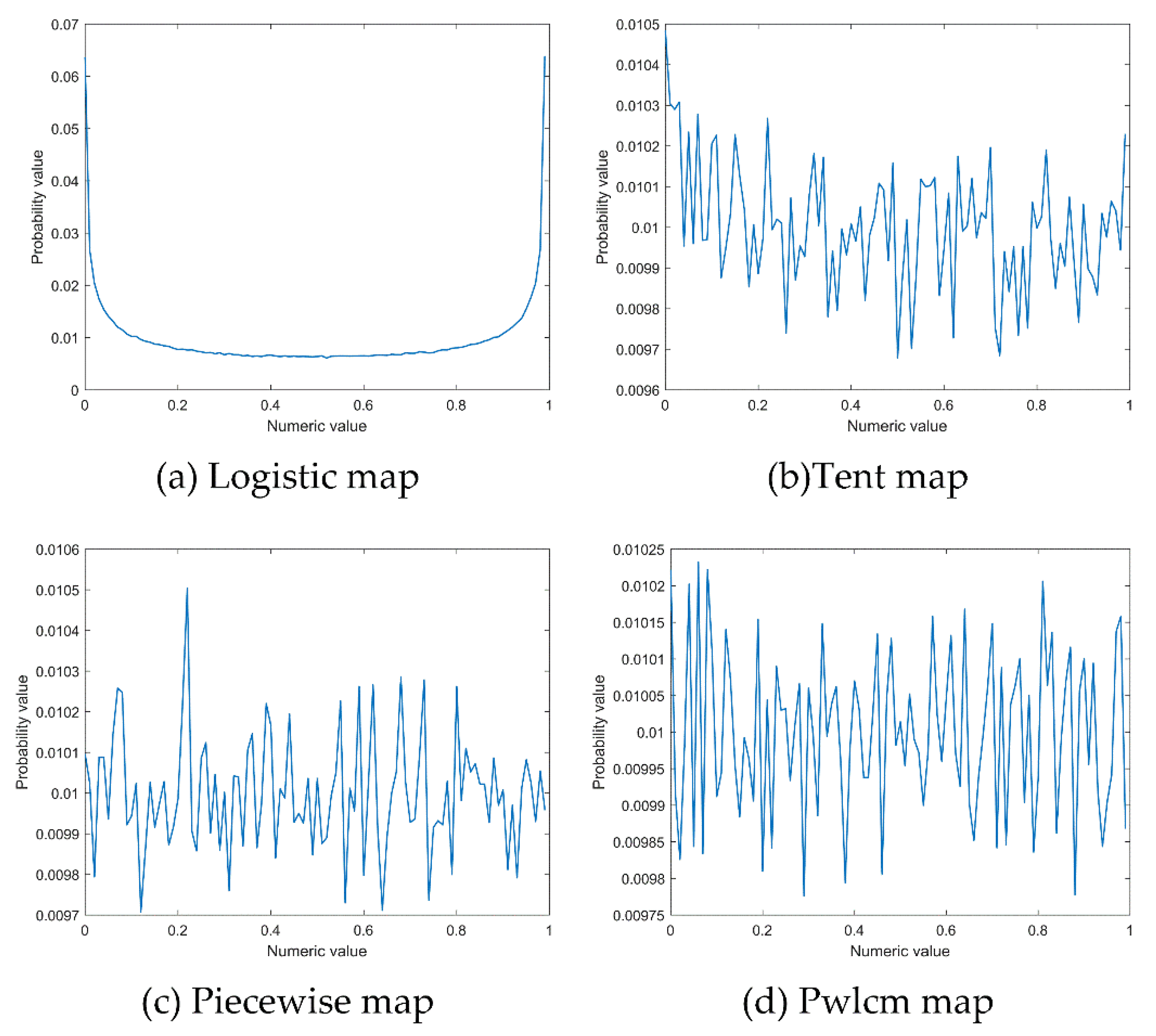
In order to intuitively display the characteristics of the four chaotic maps in Table 2, their probability distribution characteristics in the (0,1) interval are compared. Among them, the probability distribution is obtained in the following way: 50,000 chaotic numerical points generated by 50,000 iterations of chaotic mapping are used to count the probability of these 50,000 points falling into 100 intervals after equal division of interval (0,1), and the probability distribution diagram as shown in Figure 7 is drawn.

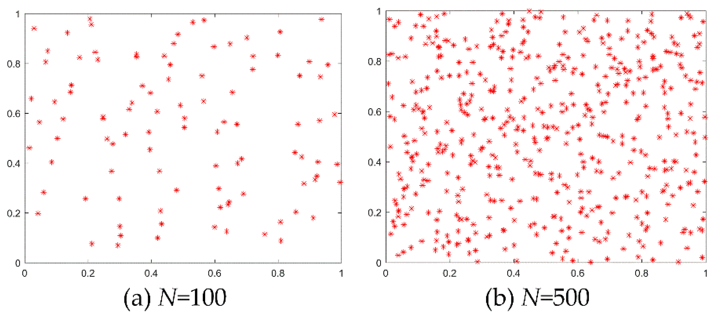
Analysis of Figure 7 shows that the logistic map shows a distribution trend that is large in the middle and small at both ends. If the global optimal solution of the function problem is distributed in the middle, there will be a large number of invalid searches, which will be very unfavorable for the global optimization. The probability distribution in the interval of the Tent map, the Piecewise map and the Pwlcm map (0,1) is uniform. The population initialized with these three distributions is evenly distributed in the solution space, so it can avoid excessive search in some local areas (such as the logistic map, a large number of searches are concentrated at both ends of the interval) and reduce the adverse impact caused by the incompatibility between the distribution characteristics of chaotic sequence and the location of the global optimal solution of the optimization problem. As can be seen from the figure, the probability fluctuation range of the Tent map is (0.0105, 0.00967), the probability fluctuation range of the Piecewise map is (0.0105, 0.0097), and the probability fluctuation range of the Pwlcm map is (0.01023, 0.00977). Compared with the Tent map and the Piecewise map, the probability distribution of the Pwlcm map is more uniform, and the interval size of the Pwlcm map probability distribution is 0.00046, which is much smaller than the other two sequences. As shown in Figure 8, if we use the Pwlcm map to initialize two two-dimensional populations with population numbers of 100 and 500 between (0, 1), it is obvious that compared with the randomly generated initial population in Figure 5, the distribution of the initial population generated by the Pwlcm map is more uniform, which is conducive to the complete search of the whole region in the initial stage of the algorithm. Therefore, this paper selects the Pwlcm map to initialize the individual population of the WPA.

After the chaotic ergodic sequence $z$ is obtained by the Pwlcm map search, the chaotic ergodic sequence $z$ needs to be transformed to the original solution space according to the following Equation (11).

$$X_i^0=lb+z_i·\left(ub-lb\right)$$

(11)

Among them, $ub$ and $lb$ represent the upper boundary and lower boundary of wolf $i$ activity, respectively.

4.1.2. Random Walk Based on Drunken Walk Model

Random walk [37] was put forward by Pearson in 1905. It is a random and irregular form of movement, and the next step in the movement process is uncertain. The idea of random walk is that an element starts random motion from any point, and after a certain period of time, it will traverse the entire space. Random walk has been widely used in many fields because of its strong applicability. Gupta et al. [38] designed an improved gray wolf optimization algorithm based on the idea of random walk, which shows good performance in solving continuous optimization problems and real-life optimization problems. Random walk can generally be divided into three types: Markov chain [39], Levy flight [40] and drunkard walk [41]. The drunk walking model is shown in Equation (12). In this model, the direction of each step of the drunk is in any direction in the whole space, which has great uncertainty and randomness and can better traverse the whole space.

$$\{\begin{array}{c}{x}_{id}^{k+1}=x_{id}^k+step·\sin {\theta }_p\\ {\theta }_p=\left(2·rand-1\right)\pi \end{array}$$

(12)

Therefore, in order to enhance the breakthrough ability of the scout wolf and avoid it falling into local areas, a walking behavior based on drunk walking is designed by combining drunk walking with greedy walking behavior, as shown in Figure 9. Equation (12) is the mathematical expression of the random walk based on the drunken walk model. In the process of wandering, scout wolf $i$ takes a greedy strategy according to Equation (12), advances one step in $h$ directions, respectively, records the position and corresponding fitness value before and after each step and then returns to the original position. Among the $h$ directions, the direction with the largest odor concentration and greater than the current odor concentration $Y_i$ is taken as the update direction of the scout wolf.

The step length $step$ of a drunk can be fixed or changed. A small step length is helpful to carry out a fine search, while a large enough step length is helpful to expand the search range or jump out of the local optimum. At the same time, considering the spatial distance between the position of the scout wolf and the lead wolf, the walking length is designed as the adaptive step length shown in Equation (13). The adaptive step length can effectively increase the randomness of the wolf search to enhance the ability of wolf breakthrough and optimization.

$$step=rand·norm\Vert x_i-g\parallel$$

(13)

$x_i$ is the position of wolf $i$, and $g$ is the position of the lead wolf.

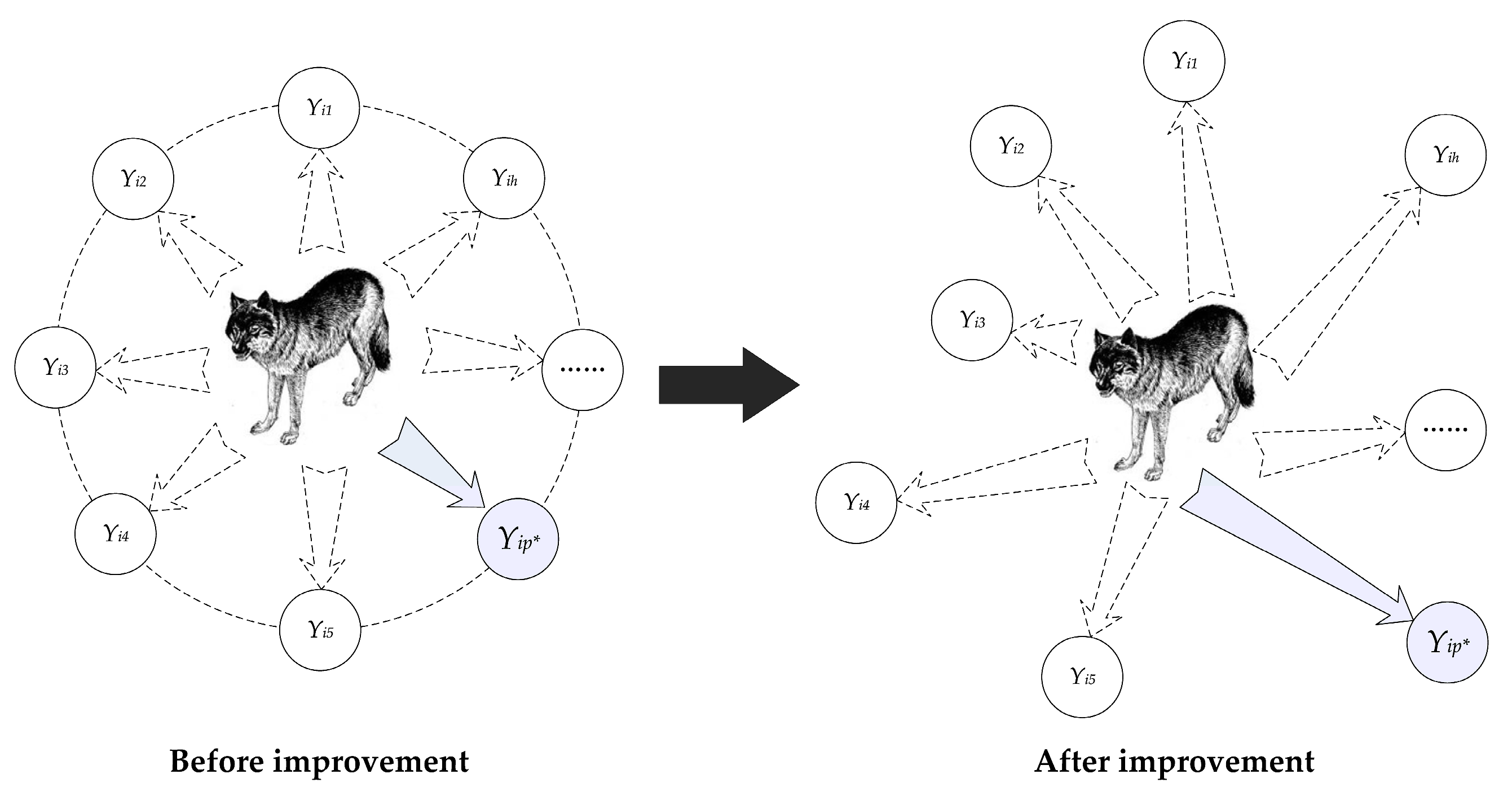
4.1.3. Half-Population Siege Strategy

The $N-1$ wolves except the lead wolf are regarded as fierce wolves, and fierce wolves quickly approach the lead wolf after receiving the summoning order. When the distance between more than half of the fierce wolves and the lead wolf is less than the determined distance $L_{near}$, all the fierce wolves will adjust their positions to be within the siege range to execute the siege behavior.

In the $k^{th}$ iteration, the maximum distance between the $N/2$ fierce wolves closest to the lead wolf and the lead wolf is $L_{Ig}^k$. In order to obtain the distance $L_{Ig}^k$, the distance between the fierce wolf and the lead wolf is sorted, and $ord\left(L_{ig}^k\right)$ represents the order of $L_{ig}^k$ in the sequence after the distance between each fierce wolf and the lead wolf is arranged in ascending order. The sequence encoding vector $P^k$ of all wolves is shown in Equation (14).

$$P^k=ord\left(L_{1g}^k\right),ord\left(L_{2g}^k\right),\dots ,ord\left(L_{ig}^k\right),\dots ,ord\left(L_{\left(N-1\right)g}^k\right)$$

(14)

In each iteration, when the maximum distance $L_{Ig}^k$ between the $N/2$ fierce wolves closest to the lead wolf and the lead wolf is less than $L_{near}$ (i.e., the siege conditions in Equation (15) are met), all fierce wolves adjust their positions and execute the siege behavior; Otherwise, they continue to perform the summoning behavior.

$$\{\begin{array}{c}ord\left(L_{ig}^k\right)=N/2\\ L_{Ig}^k\le L_{near}\end{array}$$

(15)

4.1.4. Evolutionary Mechanism Based on Hamming Distance

After several iterations of the WPA, most individual wolves are near the current optimal solution. As the similarity between individuals increases and the population diversity decreases, it is very easy to cause “stopping evolution prematurely”, leading to the stagnation of evolution. Therefore, this paper introduces the similarity judgment mechanism based on the Hamming Distance [42] to dynamically update the population in order to maintain the continuous evolution of the population. When the number of stagnant changes of the optimal value exceeds the preset threshold, we will calculate the the Hamming Distance between each wolf and the lead wolf to judge the similarity between individuals, eliminate the individual wolves with high similarity with the lead wolf and generate new individuals with low similarity with the lead wolf to enhance the diversity of the population to improve the ability of the algorithm to jump out of the local extreme value in the iteration and maintain the vitality of continuous evolution.

The Hamming Distance is mainly used to describe the difference between two vectors with the same dimension. As shown in Equation (16), the Hamming Distance is the sum $L_{ij}$ of the number of positions with different values at all corresponding positions of vector $X_i=\left(x_{i1},x_{i2},\dots ,x_{iD}\right)$ and vector $X_j=\left(x_{j1},x_{j2},\dots ,x_{jD}\right)$. It can accurately reflect the difference between two vectors, so as to objectively judge the similarity of vectors.

$$L_{ij}={\displaystyle \sum }_{d=1}^D{x}_{id}\oplus x_{jd}$$

(16)

In the above equation, $\oplus$ is the XOR operator, $D$ represents the dimension of the vector, and $d\in 1,2,\dots ,D$.

Suppose the similarity between individuals in the wolf pack is $S$, which represents the proportion of the sum of the number of dimensions with the same position in all the corresponding dimensional spaces of the two artificial wolves to the total dimension. Then, according to Equation (17), the similarity $S_{ij}$ of any two wolves in the wolf pack can be calculated. By contrast, if the calculated similarity $S_{ij}$, is less than the preset threshold $S_t$, it indicates that the similarity between the two individuals is low. Otherwise, the similarity between the two individuals is high.

$$S_{ij}=1-\frac{L_{ij}}{D}$$

(17)

When the population evolution is found to be stagnant in the iterative optimization process, the similarity between all individual wolves and the current alpha wolf is calculated by the Hamming Distance. Individuals with low similarity will be retained, individuals with high similarity will be eliminated, and individuals with low similarity to the head wolf will be generated to update the wolf group. Then the wolves are distributed in the solution space, and the global optimization ability of the algorithm is increased. The specific process is as follows:

Step 1: Calculate the similarity $S$ between all individual wolves and the lead wolf. Individuals whose $S$ is greater than $S_t$ form wolf pack $P_d$, and other individuals form wolf pack $P_x$. Let the scale of $P_d$ be $N_d$, then the scale of $P_x$ be $N-N_d$.

Step 2: In order to maintain the dominance of the population, only $r$ outstanding individuals in the wolf pack $P_d$ are retained, $r\in \left[\left(1-1/\beta \right)N_d,\left(1-1/\left(2\beta \right)\right)N_d\right]$, and the remaining individuals in $P_d$ are eliminated.

Step 3: In the optimization space, $R$ individuals whose similarity meets the requirements are randomly generated and supplemented to $P_d$, $R=\left[N_d/\left(2\beta \right),N_d/\beta \right]$.

Step 4: Combine $P_x$ and $P_d$ to form a new wolf pack, that is, the initial wolf pack $P_0$ of the next iteration.

It should be noted that wolves have good distribution in the solution space at the initial stage of evolution. In order to improve the convergence of the algorithm, save computing resources and reduce computing time, only when the population stagnant evolution algebra reaches the threshold can the population be updated by the population dynamic update method based on the Hamming Distance.

4.2. Basic Process of Improved WPA

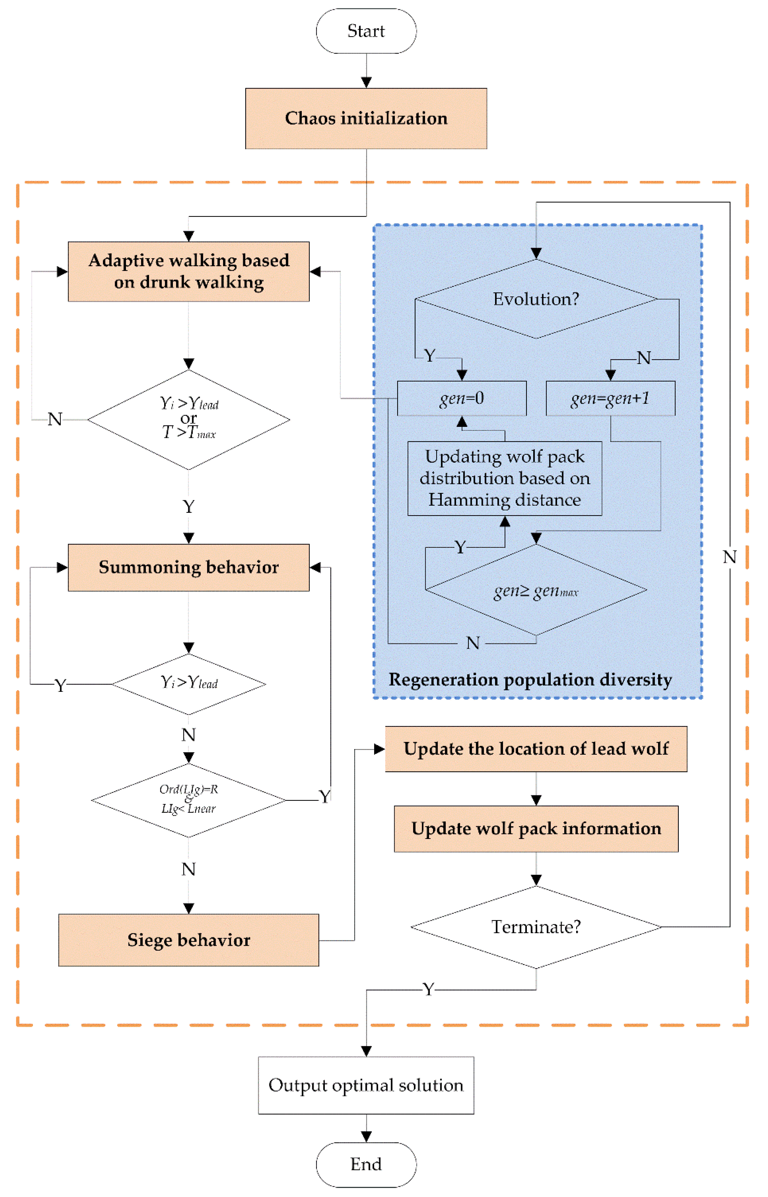
The flow of the improved algorithm is shown in Figure 10. The calculation steps of the algorithm are described below by taking the solution of the maximum value as an example:

Step 1: Initialization. According to the wolf pack generation method based on the Pwlcm map in Equation (11), $N$ artificial wolves are randomly generated in the Euclidean space of $N\times D$, with the position of artificial wolf $i$ as $X_i$, the step length factor as $S$, the maximum number of walks as $T_{max}$, the distance judgment factor as $\omega$, the maximum number of iterations as $k_{max}$, the update scale factor as $\beta$, the evolution stop threshold as $ge{n}_{max}$ and the similarity judgment threshold as $S_t$.

Step 2: Wandering behavior. Select the lead wolf and treat all other wolves except the lead wolf as scout wolves. Let all scout wolves have random walk based on the exploration direction of the drunk walk model, then decide the best position in the next step and move forward by using the adaptive greedy mechanism, calculate the fitness value of the scout wolves’ positions and update the lead wolf in real time.

Step 3: Summoning behavior. All other wolves except the lead wolf are considered fierce wolves. After the lead wolf issues the summoning command, all scout wolves quickly move closer to the lead wolf according to Equation (6). If the fierce wolf $i$ finds a better fitness value than the position of the lead wolf during the attack, that is: $Y_i\ge Y_{lead}$, then the fierce wolf $i$ replaces the lead wolf and initiates a call; otherwise, continue to attack until the siege conditions of half the population are met, end the summoning behavior and turn to Step 4.

Step 4: Siege behavior. The position of the lead wolf is regarded as the position of the prey, and all wolves besiege the prey according to Equation (9).

Step 5: Wolf pack update. Compare the objective function value $Y_{max}^{k+1}$ corresponding to the lead wolf after each iteration with the function value $Y_{lead}^k$ corresponding to the lead wolf in the previous generation. If $Y_{max}^{k+1}\ge Y_{lead}^k$, update the position of the lead wolf, and update the $R$ wolves with poor fitness value according to Equation (11).

Step 6: Determine whether to terminate. Judge whether the maximum number of iterations $k_{max}$ or the accuracy requirement is reached, and if so, output the optimal solution and its corresponding fitness value; otherwise, go to step 7.

Step 7: Determine whether to update the wolf pack. If there is no artificial wolf with a new optimal position in the current generation of the wolf pack, record the algebra $gen$ that has stopped evolving, and determine whether the conditions for updating the population are met. If $gen>ge{n}_{max}$, go to step 8; otherwise, go to step 2.

Step 8: Population update. By updating the individuals with high similarity to the lead wolf in the population based on the Hamming Distance, a new wolf pack is obtained, which is used as the initial population for the next generation evolution, then $gen=0$, and go to step 2.

4.3. Time Complexity Analysis of the Algorithm

In order to illustrate the operation efficiency of the DCWPA, this paper uses the time complexity analysis method in [43] to analyze the time complexity of the proposed algorithm.

In the WPA, the population size is $N$, and the length of individual wolf positions is $m$. The setting time of parameters such as basic motion step $step$, maximum walking period $T_{max}$ of wolf detection, siege judgment distance $L_{near}$ and update scale factor $\beta$ is ${\eta }_0$, the time of generating the initial population is ${\eta }_1$, and the time of calculating the fitness function value is $f\left(m\right)$, then the time complexity of algorithm initialization is:

$$o\left({\eta }_0+N\left(m{\eta }_1+f\left(m\right)\right)\right)=o\left(m\right)$$

(18)

If we assume the time consumption of the competition process of the lead wolf as ${\eta }_2$, the time consumption of the wandering process of the scout wolf as ${\eta }_3$, the time consumption of the fierce wolf performing the calling behavior and approaching the lead wolf as ${\eta }_4$, the time consumption of the fierce wolf moving towards the lead wolf in each dimension space as ${\eta }_5$, and the time consumption of judging whether to end the calling behavior as ${\eta }_6$, then the time complexity of the algorithm in this stage is:

$$o\left(N\left({\eta }_2+{\eta }_3+{\eta }_4+n{\eta }_5+{\eta }_6\right)\right)=o\left(m+f\left(m\right)\right)$$

(19)

From the above, the time complexity of each iteration in the WPA is:

$$T_m=o\left(m\right)+o\left(m+f\left(m\right)\right)=o\left(m+f\left(m\right)\right)$$

(20)

We put the time complexity of the algorithm analyzed in combination with the basic process of the DCWPA. In the initialization phase of the algorithm, the time consumption of generating the initialization population by chaotic mapping is $t_1$, and the other initialization processes are the same as the WPA. Therefore, the time complexity of DCWPA initialization is:

$$o\left({\eta }_0+N\left(n{\eta }_1+f\left(n\right)+t_1\right)\right)=o\left(n\right)$$

(21)

The time consumption of calculating the adaptive walk step length of the scout wolf as ${\eta }_7$, the time consumption of judging whether the siege condition of half the population is reached as ${\eta }_8$, the time consumption of population diversity detection and population evolution update as ${\eta }_9$, and the rest of the process is the same as that of the WPA. Then the time complexity of this stage is:

$$o\left(N\left({\eta }_2+{\eta }_3+{\eta }_4+n{\eta }_5+{\eta }_6+{\eta }_7+{\eta }_8+{\eta }_9\right)\right)=o\left(\mathrm{n}+f\left(n\right)\right)$$

(22)

In summary, the time complexity of each iteration process in the DCWPA is:

$$o\left(n\right)+o\left(n+f\left(n\right)\right)=o\left(n+f\left(n\right)\right)$$

(23)

Therefore, compared with the WPA, the time complexity of the DCWPA does not change, and the operating efficiency of the algorithm does not decrease.

5. Algorithm Performance Test

5.1. Benchmark Function

In order to verify the effectiveness and feasibility of the algorithm in this paper, the DCWPA and six swarm intelligence optimization algorithms are used to optimize eight Benchmark functions [44] with different mathematical characteristics and dimensions in

Table 3. Benchmark functions in experiments.

No.	Trait	Functions	Formulation	Range	Min
F1	UN	Easom	$f\left(X\right)=-\cos \left(x_1\right)·\cos \left(x_2\right)·e^{\left(-{\left(x_1-\pi \right)}^2-{\left(x_2-\pi \right)}^2\right)}$	${\left[-10,10\right]}^2$	−1
F2	UN	Matyas	$f\left(X\right)=0.26\left(x_1{}^2+x_2{}^2\right)-0.48x_1{x}_2$	${\left[-10,10\right]}^2$	0
F3	US	Sumsquares	$f\left(X\right)={\displaystyle {\displaystyle \sum }_{i=1}^D}i·{\left(x_i\right)}^2$	${\left[-10,10\right]}^D$	0
F4	US	Sphere	$f\left(X\right)={\displaystyle {\displaystyle \sum }_{i=1}^D}{x}_i{}^2$	${\left[-1.5,1.5\right]}^D$	0
F5	MS	Booth	$f\left(X\right)={\left(x_1+2x_2-7\right)}^2+{\left(2x_1+x_2-5\right)}^2$	${\left[-10,10\right]}^2$	0
F6	MS	Quadric	$f\left(X\right)={\displaystyle {\displaystyle \sum }_{i=1}^D}{\left({\displaystyle {\displaystyle \sum }_{k=1}^i}{x}_k\right)}^2$	${\left[-30,30\right]}^D$	0
F7	MN	Bohachevsky3	$f\left(X\right)=x_1{}^2+2x_2{}^2-0.3\cos \left(3\pi x_1+4\pi x_2\right)+0.3$	${\left[-100,100\right]}^2$	0
F8	MN	Eggcrate	$f\left(X\right)=x_1{}^2+x_2{}^2+25\left({\sin }^2{x}_1+{\sin }^2{x}_2\right)$	${\left[-2\pi ,2\pi \right]}^2$	0

. US and UN in trait column in Table 3 are single-peak separable and non-separable functions, respectively, while MS and MN are multi-peak separable and multi-peak non separable functions, respectively. Here, the unimodal function is mainly used to test the local exploration ability of the algorithm, the multi-modal function is mainly used to test the global search ability of the algorithm, and the higher-dimension and non-separable function is mainly applied to test the performance of the algorithm to solve complex functions.

5.2. Parameter Setting

The comparison algorithms in this paper are the WPA, the opposite wolf pack algorithm (OWPA) [45], the cultural wolf pack algorithm (CWPA) [46], PSO, ABC and ASFA. Due to the differences in the test parameters adopted by the intelligent evolutionary algorithm in different reference, this paper selects the same setting of general parameters; that is, the maximum number of iterations is 200, the initial population size is 50, and the other parameter settings are shown in

Table 4. Parameter setting of the intelligent optimization algorithms.

Methods	Parameter Setting
PSO	$\omega =0.7298$, $c_1=c_2=1.4946$, ${\mathrm{limit}}_v\in \left(-0.5,0.5\right)$
ABC	$N=2$, $\mathrm{limit}=100$
ASFA	$tr{y}_{num}=100$, $v=1$, $de=0.618$, $step=0.1$
WPA	$T_{max}=10$, $S=0.06$, $\omega \omega =0.04$, $\beta =5$
OWPA	$T_{max}=10$, $S=0.06$, $\omega \omega =0.04$, $\beta =5$
CWPA	$T_{max}=10$, $S=0.06$, $\omega \omega =0.04$, $\beta =5$
DCWPA	$T_{max}=10$, $S=0.06$, $\omega \omega =0.04$, $\beta =5$

.

5.3. Analysis of Simulation Results

The above seven intelligent algorithms are used to conduct 20 independent experiments on the eight typical test functions shown in Table 3. The simulation experiment environment is as follows: HONOR Magic Book Pro, WIN10 operating system, Intel corei5-10210U processor, the program is implemented in MATLAB R2019b, m language. In this paper, the optimal value (BEST), worst value (WORST), mean value (MEAN) and standard deviation (STD) of the objective function, optimization success rate (SR) and average optimization success evolution number (AEN) are used to evaluate the pros and cons of the algorithm [47].

Table 5. Comparison of test results of the intelligent optimization algorithms.

FUN	Dim	Index	PSO	ABC	AFSA	WPA	OWPA	CWPA	DCWPA
F1	2	BEST	−1	−1	−1	−1	−1	−1	−1
		MEAN	−1	−1	−0.701	−0.95	−0.9999	−0.9999	−1
		WORST	−1	−1	−8.06 × 10−5	−8.11 × 10−5	−0.9997	−0.9998	−1
		STD	7.8644 × 10−5	0	0.4678	0.2236	7.6544 × 10−5	5.8551 × 10−5	2.1721 × 10−8
		SR	100%	100%	0	95%	10%	25%	100%
		AEN	200	37.4	200	200	200	200	200
F2	2	BEST	7.9904 × 10−11	9.6388 × 10−7	6.7805 × 10−9	3.6266 × 10−20	2.9776 × 10−22	1.8871 × 10−14	1.3166 × 10−23
		MEAN	4.4123 × 10−8	2.0856 × 10−4	9.2214 × 10−7	1.8457 × 10−17	1.2073 × 10−16	6.0856 × 10−7	4.4866 × 10−20
		WORST	2.4008 × 10−7	8.5121 × 10−4	1.3451 × 10−5	1.1829 × 10−16	1.1454 × 10−15	5.2634 × 10−6	5.1666 × 10−19
		STD	5.9306 × 10−8	2.418 × 10−4	2.9783 × 10−6	3.2654 × 10−17	2.8883 × 10−16	1.1774 × 10−6	1.2333 × 10−19
		SR	100%	20%	95%	100%	100%	100%	100%
		AEN	12.2	175.25	133.8	19.6	13.95	32.3	4.85
F3	150	BEST	476.9659	8.9914 × 104	1.5141 × 104	1.4595 × 10−11	15.1564	8.0471 × 10−7	5.0886 × 10−12
		MEAN	633.0432	1.133 × 105	1.6486 × 104	2.5592 × 10−9	40.8419	0.262	9.8624 × 10−10
		WORST	750.0193	1.3107 × 105	1.7742 × 104	1.6101 × 10−8	158.2036	5.1268	8.005 × 10−9
		STD	66.4026	1.1949 × 104	703.0988	4.1411 × 10−9	29.0761	1.1453	2.0005 × 10−9
		SR	0	0	0	100%	0	65%	100%
		AEN	200	200	200	134.8	200	192.35	142.9
F4	200	BEST	11.8498	57.257	451.6054	6.2244 × 10−15	0.0525	3.7845 × 10−10	1.5957 × 10−15
		MEAN	16.2412	65.6567	473.3768	6.8221 × 10−13	0.0936	4.7262 × 10−9	2.532 × 10−13
		WORST	19.2437	74.0817	493.5115	5.3258 × 10−12	0.1488	3.7217 × 10−8	1.236 × 10−12
		STD	2.0312	4.9783	10.3599	1.2832 × 10−12	0.03	8.2814 × 10−9	3.9012 × 10−13
		SR	0	0	0	100%	0	100%	100%
		AEN	200	200	200	82.85	200	117.7	92.45
F5	2	BEST	3.4468 × 10−8	5.7334 × 10−12	1.1403 × 10−6	2.8894 × 10−7	4.0935 × 10−8	1.2224 × 10−7	6.1414 × 10−17
		MEAN	1.4946 × 10−6	1.1554 × 10−10	1.3081 × 10−5	2.3196 × 10−6	6.5075 × 10−6	1.0868 × 10−5	1.3109 × 10−10
		WORST	9.3532 × 10−6	6.0774 × 10−10	4.5909 × 10−5	1.1638 × 10−5	1.5391 × 10−5	9.7972 × 10−5	2.4185 × 10−9
		STD	2.1951 × 10−6	1.6551 × 10−10	1.4181 × 10−5	2.4271 × 10−6	3.6939 × 10−6	2.1291 × 10−5	5.3893 × 10−10
		SR	100%	100%	50%	95%	90%	65%	100%
		AEN	65.3	88.55	167.05	52.45	106.7	122.15	18.25
F6	100	BEST	15.0907	1.396 × 104	2.2416 × 10−5	6.9983 × 10−11	1.0112 × 103	2.3952 × 10−6	9.9569 × 10−12
		MEAN	25.9454	2.7012 × 104	2.2547	2.817 × 10−8	3.3495 × 103	0.6243	2.7455 × 10−9
		WORST	42.8016	3.4634 × 104	35.0245	1.9521 × 10−7	1.2198 × 104	12.4852	2.7331 × 10−8
		STD	6.9341	4.6356 × 103	7.9096	5.337 × 10−8	2.3253 × 103	2.7918	6.5291 × 10−9
		SR	0	0	0	100%	0	20%	100%
		AEN	200	200	200	149.65	200	198.8	134.05
F7	2	BEST	3.5387 × 10−7	9.6579 × 10−7	0.0039	3.1742 × 10−10	8.3267 × 10−16	3.967 × 10−9	0
		MEAN	6.6341 × 10−6	7.0323 × 10−5	701.6509	0.5579	0.1808	0.6211	2.6368 × 10−16
		WORST	7.8543 × 10−5	4.5012 × 10−4	7.2342 × 103	0.9399	2.0327	0.9412	2.8311 × 10−15
		STD	1.7217 × 10−5	1.0936 × 10−4	1.5802 × 103	0.3904	0.4839	0.3834	6.507 × 10−16
		SR	90%	35%	0	20%	75%	10%	100%
		AEN	106.4	158.3	200	193.95	87.05	193.85	12.8
F8	2	BEST	1.0388 × 10−6	4.639 × 10−20	4.8442 × 10−5	4.4745 × 10−19	1.1689 × 10−18	3.6379 × 10−13	5.3206 × 10−21
		MEAN	1.2549 × 10−5	5.0131 × 10−18	2.8511	5.802 × 10−16	0.9488	4.2246 × 10−4	2.7143 × 10−18
		WORST	5.5292 × 10−5	2.1425 × 10−17	9.4893	5.525 × 10−15	9.4882	0.0021	1.9367 × 10−17
		STD	1.2975 × 10−5	5.6373 × 10−18	4.4582	1.2884 × 10−15	2.9204	5.669 × 10−4	4.4522 × 10−18
		SR	65%	100%	0	100%	90%	30%	100%
		AEN	150.2	23.35	200	37.4	48.05	155.6	4.2

shows the comparison results of the seven algorithms for the simulation calculation of the test function.

In order to visually show the performance of each algorithm, Figure 11 shows the radar chart comparing the obtained indicators. The closer the corresponding point of each index is to the center, the better the performance of the algorithm on this index is and vice versa. The area of the closed image composed of each color can represent the overall performance of the algorithm; that is, the smaller the area, the better the overall performance of the algorithm.

From Table 5 and Figure 11, it can be seen that compared with other algorithms, the BEST, MEAN, WORST, STD and AEN obtained by the DCWPA are all better. The DCWPA shows better performance. The detailed analysis is as follows:

(1)

The DCWPA has strong global search ability. For high-dimensional functions, the complexity of problem solving will increase exponentially as the spatial dimension of the solution increases, that is, to cause the “dimensional disaster” in computing. The six algorithms, PSO, ABC, ASFA, WPA, OWPA, and CWPA, have good calculation results for 2-dimensional and low-dimensional functions, but it is difficult to successfully optimize the multi-dimensional and multi-modal functions F6. However, the DCWPA not only performs well for low-dimensional functions, but also performs better for high-dimensional complex functions, indicating that the DCWPA has a very strong ability to jump out of local optima.

(2)

The DCWPA has good local exploration ability. When the classical algorithms PSO, ABC and ASFA are used to solve the low-dimensional, multimodal function F4, they cannot find a solution that meets the accuracy requirements, and generally fall into local optimum. The WPA, the OWPA and the CWPA are not good for solving F1 except that the success rate of solving the unimodal function F2 is 100%, and the accuracy of the solution is high. The optimization success rate of the DCWPA for eight functions is 100%, indicating that the DCWPA is applicable to most functions. The DCWPA obtains a solution that meets the accuracy requirements for each function with a small number of iterations, and the solution accuracy is much higher than other algorithms, and even the solution results for F1 and F7 are the most optimal in theory.

(3)

The DCWPA has high solution efficiency. In the 20 solving calculations, except that the average number of iterations for solving the low-dimensional, unimodal function F1 reaches 200 and is lower than only ABC, the average number of iterations for solving all other functions is smaller than that of other algorithms to obtain solutions that meet the accuracy requirements.

(4)

The DCWPA has good robustness. It can be seen from the solution results of the eight standard test functions that the variance of the DCWPA is the smallest, and the stability of the DCWPA is stronger than other algorithms.

In order to further analyze the performance of the proposed algorithm, Figure 12 shows the comparison of the average convergence curves of the seven algorithms for solving eight functions, respectively.

It can be seen from Figure 12 that the convergence speed and solution accuracy of the seven algorithms for Easom function are generally higher than other functions. As a whole, PSO, ABC, ASFA and CWPA converge faster, but the effect of solving high-dimensional complex functions is far from satisfactory and the continuous evolution ability is weak, which are easy to fall into local optimization. In the process of iteration, the accuracy of the results obtained by the OWPA and the WPA is constantly improving; it is not easy to fall into local optimization, and it is even possible to find the optimal solution, which shows the advantages of the wolf pack algorithm in solving complex functions, but the convergence speed of the algorithm is slow, and the solution efficiency is low. The average convergence curve of the DCWPA is the straight line with the largest change speed and the smallest final function value, which shows that the DCWPA has not only the fastest convergence speed, the highest solution efficiency, but also the highest solution accuracy and the strongest optimization ability in the solution of eight functions.

To sum up, in the aspects of global search efficiency, convergence speed and local development accuracy, the DCWPA has the best performance with better optimization effects than that of the other six algorithms. It shows the effectiveness of the algorithm improvement strategy for solving complex functions in continuous space.

6. Parameter Identification of the PV Module Model

6.1. Effectiveness and Feasibility Test

To verify its effectiveness in parameter identification, the DCWPA is used to extract parameters for SDM, DDM and PV module models. The measured data of the current (I) and voltage (V) of the three models are all from reference [48]. All the parameter settings and the experimental environment are the same as those in Section 4 of this paper, except that the maximum number of iterations for each calculation is set to 2000. The objective functions of the three models are calculated 20 times independently by using the DCWPA. The obtained I–V features and related experimental data are shown in

Table 6. Simulation results of using the DCWPA for three models solution.

SDM				DDM				PV
${\mathit{V}}_{\mathit{m}} \left(\mathbf{V}\right)$	${\mathit{I}}_{\mathit{m}} \left(\mathbf{A}\right)$	${\mathit{I}}_{\mathit{c}} \left(\mathbf{A}\right)$	$\mathit{D}(\mathbf{\%})$	${\mathit{V}}_{\mathit{m}} \left(\mathbf{V}\right)$	${\mathit{I}}_{\mathit{m}} \left(\mathbf{A}\right)$	${\mathit{I}}_{\mathit{c}} \left(\mathbf{A}\right)$	$\mathit{D}(\mathbf{\%})$	${\mathit{V}}_{\mathit{m}} \left(\mathbf{V}\right)$	${\mathit{I}}_{\mathit{m}} \left(\mathbf{A}\right)$	${\mathit{I}}_{\mathit{c}} \left(\mathbf{A}\right)$	$\mathit{D}(\mathbf{\%})$
−0.2057	0.764	0.7640	−0.0003	−0.2057	0.764	0.7639	−0.0087	0.1248	1.0315	1.0295	−0.1986
−0.1291	0.762	0.7626	0.0788	−0.1291	0.762	0.7625	0.0720	1.8093	1.03	1.0276	−0.2356
−0.0588	0.7605	0.7613	0.1075	−0.0588	0.7605	0.7613	0.1023	3.3511	1.026	1.0258	−0.0187
0.0057	0.7605	0.7601	−0.0474	0.0057	0.7605	0.7601	0.0512	4.7622	1.022	1.0241	0.2019
0.0646	0.76	0.7591	−0.1235	0.0646	0.76	0.7590	−0.1260	6.0538	1.018	1.0222	0.4081
0.1185	0.759	0.7581	−0.1228	0.1185	0.759	0.7581	−0.1243	7.2364	1.0155	1.0197	0.4159
0.1678	0.757	0.7571	0.0178	0.1678	0.757	0.7571	0.0173	8.3189	1.014	1.0161	0.2087
0.2132	0.757	0.7569	−0.1058	0.2132	0.757	0.7562	−0.1055	9.3097	1.01	1.0102	0.0244
0.2545	0.7555	0.7552	−0.0454	0.2545	0.7555	0.7552	−0.0447	10.2163	1.0035	1.0004	−0.3069
0.2924	0.754	0.7537	−0.0343	0.2924	0.754	0.7537	−0.0335	11.0449	0.988	0.9844	−0.3621
0.3269	0.7505	0.7515	0.1293	0.3269	0.7505	0.7515	0.1298	11.8018	0.963	0.9595	−0.3627
0.3585	0.7465	0.7474	0.1241	0.3585	0.7465	0.7474	0.1238	12.4929	0.9255	0.9229	−0.2762
0.3873	0.7385	0.7402	0.2264	0.3873	0.7385	0.7402	0.2251	13.1231	0.8725	0.8728	0.0347
0.4137	0.728	0.7274	−0.0812	0.4137	0.728	0.7274	−0.0836	13.6983	0.8075	0.8075	0.0035
0.4373	0.7065	0.7070	0.0657	0.4373	0.7065	0.7069	0.0625	14.2221	0.7265	0.7286	0.2872
0.459	0.6755	0.6752	−0.0391	0.459	0.6755	0.6752	0.0425	14.6995	0.6345	0.6373	0.4460
0.4784	0.632	0.6307	−0.2078	0.4784	0.632	0.6307	−0.2105	15.1346	0.5345	0.5363	0.3382
0.496	0.573	0.5718	−0.2017	0.496	0.573	0.5718	−0.2025	15.5311	0.4275	0.4295	0.4681
0.5119	0.499	0.4995	0.1058	0.5119	0.499	0.4995	0.1081	15.8929	0.3185	0.3187	0.0517
0.5265	0.413	0.4136	0.1432	0.5265	0.413	0.4136	0.1497	16.2229	0.2085	0.2072	−0.6177
0.5398	0.3165	0.3175	0.3109	0.5398	0.3165	0.3175	0.3227	16.5241	0.101	0.0960	−4.9950
0.5521	0.212	0.2122	0.0763	0.5521	0.212	0.2122	0.0953	16.7987	−0.008	−0.0085	6.0499
0.5633	0.1035	0.1023	−1.1754	0.5633	0.1035	0.1023	−1.1448	17.0499	−0.111	−0.1110	0.0073
0.5736	−0.01	−0.0087	−13.187	0.5736	−0.01	−0.0087	−13.286	17.2793	−0.209	−0.2092	0.0890
0.5833	−0.123	−0.1255	2.0161	0.5833	−0.123	−0.1255	2.0360	17.4885	−0.303	−0.3006	−0.7882
0.59	−0.21	−0.2085	−0.7248	0.59	−0.21	−0.2085	−0.6964	-	-	-	-

, and the I–V characteristics are shown in Figure 13.

In Table 6, $V_m$ and $I_m$ are measured voltage and measured current data, respectively, $I_c$ is the current data obtained from simulation calculation, $D$ is the error rate between the simulated current and the measured current, $D=I_c/I_m-1$. The closer $D$ is to 0, the more accurate $I_c$ is. As can be seen from Table 6, when $V_m=0.5736$, the $D$ of the single-diode model and the double-diode model reach the maximum value of −13.1878% and −13.2862%, respectively. When $V_m=16.5241$ and $V_m=16.7987$, the $D$ of the PV model reaches a relatively large value of −4.9950% and 6.0499%. The results show that the simulation data of the DCWPA are highly consistent with the measured data in the whole voltage range. The practical application effect of the parameters identified by the DCWPA is more intuitively shown in Figure 13. It can also be seen from the figure that the measured and simulated I and V on the three models have a high degree of coincidence, indicating that the error of the predicted parameters in practical application is very small, and the accuracy is relatively high. In particular, the parameter identification of the double-diode model and the PV module model is more difficult than that of the single-diode model, but the DCWPA can still obtain more accurate identification results. It shows that the DCWPA can show good performance in parameter identification, and the identified parameters can be used in practical application. It is proved that the DCWPA has excellent comprehensive performance.

6.2. Stability and Robustness Test

To verify the superiority in performance, the proposed DCWPA is compared with five algorithms, ABC, IJAYA [49], PSO, crow search algorithm (CSA) [50] and the WPA. ABC, PSO, IJAYA and CSA are commonly used algorithms in the field of PV parameter identification. The overall size of all the compared algorithms is set to 100, the maximum number of iterations of the algorithms are all set to 2000, and other algorithm parameters are set in [49,50] and Section 4 of this paper. There is no completely correct solution to the parameter identification problem. The RMSE is the most important criterion for evaluating the performance of the algorithm. The smaller the RMSE value, the better the performance of the algorithm. Each algorithm is run independently for 20 times, and the obtained simulation results are shown in

Table 7. Solution results of three models by different algorithms.

Model	Index	PSO	ABC	CSA	IJAYA	WPA	DCWPA
SDM	BEST	3.1262 × 10−2	1.0140 × 10−3	2.9826 × 10−3	1.2816 × 10−3	2.3252 × 10−3	9.8745 × 10−4
	WORST	0.1004	1.2414 × 10−3	1.1751 × 10−2	1.8729 × 10−3	2.7204 × 10−3	9.9366 × 10−4
	MEAN	6.1721 × 10−2	1.1405 × 10−3	6.0005 × 10−3	1.4222 × 10−3	2.5813 × 10−3	9.9182 × 10−4
	SD	2.9675 × 10−2	8.6246 × 10−5	3.8113 × 10−3	2.5345 × 10−4	2.2205 × 10−4	2.4858 × 10−6
DDM	BEST	1.2001 × 10−2	9.9687 × 10−4	5.4739 × 10−3	1.6090 × 10−3	3.8205 × 10−3	9.8780 × 10−4
	WORST	0.2467	1.0371 × 10−3	1.3528 × 10−2	2.3040 × 10−3	3.8207 × 10−3	9.8882 × 10−4
	MEAN	0.1126	1.0038 × 10−3	9.6281 × 10−3	1.9171 × 10−3	3.8206 × 10−3	9.8831 × 10−4
	SD	9.9695 × 10−2	1.9256 × 10−5	3.0123 × 10−3	2.7273 × 10−4	5.4595 × 10−8	4.3543 × 10−7
PV	BEST	8.7645 × 10−3	2.4399 × 10−3	4.7107 × 10−3	2.4520 × 10−3	5.3838 × 10−3	2.4320 × 10−3
	WORST	1.0904	2.5122 × 10−3	8.8175 × 10−3	2.4986 × 10−3	5.3846 × 10−3	2.4331 × 10−3
	MEAN	0.5371	2.4803 × 10−3	6.8965 × 10−3	2.4682 × 10−3	5.3841 × 10−3	2.4326 × 10−3
	SD	0.3784	2.6510 × 10−5	1.7547 × 10−3	1.8621 × 10−5	4.6818 × 10−7	4.2351 × 10−7

.

Table 7 shows the best value (BEST), the worst value (WORST), the mean value (MEAN) and the standard deviation (SD) obtained by the six algorithms for optimizing the three models. It can be clearly seen from Table 7 that, except for the standard deviation of the double-diode model, which is inferior to the WPA, the rest of the indexes obtained by the DCWPA are better than those obtained by other algorithms. Especially under the condition of the same number of calculation iterations, the solution accuracy of the DCWPA is obviously better than other algorithms. It shows that the accuracy of the optimal value searched by the DCWPA algorithm on the single-diode model is higher, and the execution process of the algorithm is more stable. Compared with the five comparison algorithms, the DCWPA algorithm still has certain advantages when applied to solve practical problems, which proves that the improvement of the algorithm in this paper is practical and effective. It can be concluded that in the field of PV system parameter identification in industrial applications, the DCWPA can achieve relatively good parameter identification results, ahead of the other five comparison algorithms, proving the superior performance of the DCWPA in practical applications.

The convergence curves of the six algorithms for the three PV models are shown in Figure 14. Obviously, among the three models, the DCWPA has the fastest convergence speed, and the optimal solution is better than other algorithms. As can be seen from Figure 14, PSO converges rapidly but falls into the local optimal solution. The convergence speed of CSA is slow, and it is difficult to find the optimal value. The WPA has some advantages in solving, but its local exploration ability is weak, and the accuracy of the solution is low. IJAYA and ABC have faster convergence speed and higher accuracy, but the solution results of the two algorithms are slightly inferior to the DCWPA. The DCWPA has the fastest convergence speed and the highest solution accuracy and shows strong optimization ability.

Therefore, through the practical application of the DCWPA in PV system parameter identification, it is proved that the proposed DCWPA is effective and superior in practical production and life.

7. Conclusions

Aiming at the low accuracy problem of parameter identification by the current intelligent optimization algorithm in a PV model, this paper improves the basic wolf pack algorithm and puts forward a novel drunken adaptive walking chaotic wolf pack algorithm, which is named the DCWPA for short. The DCWPA uses the chaotic map sequence to initialize the population, thus to improve the diversity of the initial population. It adopts the walking direction mechanism based on the drunk walking model and the adaptive walking step size to increase the randomness of walking, enhance the individual’s ability to explore and develop and improve the ability of algorithm optimization. It also designs the judgment conditions for half siege in order to accelerate the convergence of the algorithm and improve the speed of the algorithm. In the iterative process, according to the change of the optimal solution, the Hamming Distance is used to judge the similarity of individuals in the population, and the individuals of the population are constantly updated to avoid the algorithm from stopping evolution prematurely due to falling into local optimization. This paper selects eight standard test functions (Benchmark) with different characteristics to verify the performance of the DCWPA algorithm for continuous optimization and uses it for parameter identification of a single-diode five-parameter model, a double-diode seven-parameter model and a photovoltaic module model. The results show that the DCWPA has stronger optimization ability in high-dimensional complex continuous reading space and can accurately and reliably identify the model parameters of photovoltaic modules. This research provides a new idea and method for solving the parameter identification problem of a PV module model.

Although the DCWPA shows better performance in PV module model parameter identification, there are still some works that need further improvement. First, whether the proposed method still has good performance for complex PV module models requires continued validation and research. In addition, in terms of the DCWPA algorithm, too many parameters and complex algorithm processes still need to be solved in the next step. Finally, the method should be further extended to other practical engineering problems.

References

1. Liu, L.; Wang, Z.; Zhang, H.; Xue, Y. Solar energy development in China—A review. Renew. Sustain. Energy Rev. 2010, 14, 301–311. [Google Scholar] [CrossRef]
2. Zhou, G.; Li, K.; Liu, W.; Su, Z. Grey wolf optimizes mixed parameter multi-classification twin support vector machine. J. Front. Comput. Sci. Technol. 2020, 14, 628–636. [Google Scholar] [CrossRef]
3. Ren, Y.; Yan, W. An efficient algorithm for high-dimensional function optimization. Soft Comput. 2013, 17, 995–1004. [Google Scholar] [CrossRef]
4. Errouha, M.; Motahhir, S.; Combe, Q.; Derouich, A. Parameters extraction of single diode PV model and application in solar pumping. In International Conference on Integrated Design and Production; Springer: Cham, Switzerland, 2019; pp. 178–191. [Google Scholar] [CrossRef]
5. Alam, D.F.; Yousri, D.A.; Eteiba, M.B. Flower pollination algorithm based solar PV parameter estimation. Energy Convers. Manag. 2015, 101, 410–422. [Google Scholar] [CrossRef]
6. Hamadi, S.A.; Chouder, A.; Rezaoui, M.M.; Motahhir, S.; Kaddouri, A.M. Improved Hybrid Parameters Extraction of a PV Module Using a Moth Flame Algorithm. Electronics 2021, 10, 2798. [Google Scholar] [CrossRef]
7. Wang, R. Parameter Identification of Photovoltaic Cell Model Based on Enhanced Particle Swarm Optimization. Sustainability 2021, 13, 840. [Google Scholar] [CrossRef]
8. Kennedy, J.; Eberhart, R. Particle swarm optimization. In Proceedings of the ICNN’95-International Conference on Neural Networks, Perth, Australia, 27 November–1 December 1995; pp. 1942–1948. [Google Scholar]
9. Li, X.L.; Shao, Z.J.; Qian, J.X. An optimization model based on animal commune: Fish swarm algorithm. Syst. Eng. Theory Pract. 2002, 22, 32–38. [Google Scholar]
10. Colorni, A.; Dorigo, M.; Maniezzo, V. Distributed optimization by ant colonies. In Proceedings of the First European Conference on Artificial Life, Paris, France, 11–13 December 1991; pp. 134–142. [Google Scholar]
11. Passino, K.M. Biomimicry of bacterial foraging for distributed optimization and control. IEEE Control Syst. Mag. 2002, 22, 52–67. [Google Scholar] [CrossRef]
12. Karaboga, D.; Basturk, B. A powerful and efficient algorithm for numerical function optimization: Artificial bee colony (ABC) algorithm. J. Glob. Optim. 2007, 39, 459–471. [Google Scholar] [CrossRef]
13. Wu, H.; Zhang, F.; Wu, L. A new swarm intelligence algorithm-wolf pack algorithm. Syst. Eng. Electron. Technol. 2013, 35, 2430–2438. [Google Scholar]
14. Chu, D.; Chen, H.; Wang, X. Whale optimization algorithm based on adaptive weight and simulated annealing. Acta Electron. Sin. 2019, 47, 992–999. [Google Scholar] [CrossRef]
15. Long, W.; Cai, S.; Jiao, J.; Wu, T.B. An improved grey wolf optimization algorithm. Acta Electron. Sin. 2019, 47, 169–175. [Google Scholar] [CrossRef]
16. Ma, W.; Sun, Z.A. Global cuckoo optimization algorithm using coarse-to-fine search. Acta Electron. Sin. 2015, 43, 2429–2439. [Google Scholar] [CrossRef]
17. Jordehi, A.R. Enhanced leader particle swarm optimisation (ELPSO): An efficient algorithm for parameter estimation of photovoltaic (PV) cells and modules. Sol. Energy 2018, 159, 78–87. [Google Scholar] [CrossRef]
18. Gong, W.; Cai, Z. Parameter extraction of solar cell models using repaired adaptive differential evolution. Sol. Energy 2013, 94, 209–220. [Google Scholar] [CrossRef]
19. Oliva, D.; Cuevas, E.; Pajares, G. Parameter identification of solar cells using artificial bee colony optimization. Energy 2014, 72, 93–102. [Google Scholar] [CrossRef]
20. Yu, K.; Qu, B.; Yue, C.; Ge, S.; Chen, X.; Liang, J.A. Performance-guided JAYA algorithm for parameters identification of photovoltaic cell and module. Appl. Energy 2019, 237, 241–257. [Google Scholar] [CrossRef]
21. Liang, J.; Ge, S.; Qu, B.; Yu, K.J. Improved particle swarm optimization algorithm for solving power system economic dispatch problem. Control Decis. 2020, 35, 1813–1822. [Google Scholar]
22. Liang, J.; Ge, S.; Qu, B.; Yu, K.; Liu, F.; Yang, H.; Wei, P.; Li, Z. Classified perturbation mutation based particle swarm optimization algorithm for parameters extraction of photovoltaic models. Energy Convers. Manag. 2020, 203, 112138. [Google Scholar] [CrossRef]
23. Jian, X.; Weng, Z. A logistic chaotic JAYA algorithm for parameters identification of photovoltaic cell and module models. Optik 2020, 203, 164041. [Google Scholar] [CrossRef]
24. Yu, K.; Liang, J.J.; Qu, B.Y.; Cheng, Z.; Wang, H. Multiple learning backtracking search algorithm for estimating parameters of photovoltaic models. Appl. Energy 2018, 226, 408–422. [Google Scholar] [CrossRef]
25. Xu, Y.; Gao, Z.; Zhu, X. Parameter identification method of photovoltaic array based on shuffled frog leaping algorithm. Actor Energy Sol. Sin. 2019, 40, 1903–1911. [Google Scholar]
26. Yang, C.; Tu, X.; Chen, J. Algorithm of marriage in honey bees optimization based on the wolf pack search. In Proceedings of the 2007 International Conference on Intelligent Pervasive Computing (IPC 2007), Jeju Island, Korea, 11–13 October 2007; pp. 462–467. [Google Scholar]
27. Wu, H.; Zhang, F.; Zhan, R.; Wang, S. A binary wolf pack algorithm for solving 0–1 knapsack problem. Syst. Eng. Electron. 2014, 36, 1660–1667. [Google Scholar]
28. Wu, H.; Zhang, F.; Li, H.; Liang, X. Discrete wolf pack algorithm for traveling salesman problem. Control Decis. 2015, 30, 1861–1867. [Google Scholar]
29. Liu, Y.L.; Li, W.M.; Wu, H.S.; Song, W.J. Track planning for unmanned aerial vehicles based on wolf pack algorithm. J. Syst. Simul. 2015, 27, 1838–1843. [Google Scholar]
30. Wang, Y.; Chen, M.; Cheng, T.; Shen, Q.; Dong, L. Research on improved Wolf pack algorithm based on kitting differential evolution. Comput. Appl. Res. 2019, 36, 2305–2310. [Google Scholar]
31. Hui, X.; Guo, Q.; Wu, P.; Zhao, Y. An improved wolf pack algorithm. Control Decis. 2017, 32, 1163–1172. [Google Scholar]
32. Yu, L.; Zhang, L.; Gu, X. Methanol synthesis mechanism modeling and parameter estimation based on improved wolf pack algorithm. J. East China Univ. Sci. Technol. 2017, 43, 815–823. [Google Scholar]
33. Zhou, J.; Tian, M.; Zhong, F. High density wireless sensor network efficient clustering method based on chaotic niche wolf algorithm. Gansu Sci. Technol. 2016, 32, 38–40. [Google Scholar]
34. Ma, L.; Lu, C.; Gu, Q.; Chen, X. Cellular wolf pack optimization algorithm for multi-objective 0–1 programming. Oper. Manag. 2018, 27, 17–24. [Google Scholar]
35. Kang, T.; Yao, J.; Jin, M.; Yang, S.; Duong, T. A Novel Improved Cuckoo Search Algorithm for Parameter Estimation of Photovoltaic (PV) Models. Energies 2018, 11, 1060. [Google Scholar] [CrossRef] [Green Version]
36. Gandomi, A.H.; Yang, X.S.; Talatahari, S.; Alavi, A.H. Firefly algorithm with chaos. Commun. Nonlinear Sci. Numer. Simul. 2013, 18, 89–98. [Google Scholar] [CrossRef]
37. Pearson, K. The problem of the random walk. Nature 1905, 72, 294. [Google Scholar] [CrossRef]
38. Gupta, S.; Deep, K. A novel random walk grey wolf optimizer. Swarm Evol. Comput. 2019, 44, 101–112. [Google Scholar] [CrossRef]
39. Norris, J.R.; Norris, J.R. Markov Chains; Cambridge University Press: Cambridgeshire, UK, 1998. [Google Scholar]
40. Viswanathan, G.M.; Afanasyev, V.; Buldyrev, S.V.; Murphy, E.J.; Prince, P.A.; Stanley, H.E. Lévy flight search patterns of wandering albatrosses. Nature 1996, 381, 413–415. [Google Scholar] [CrossRef]
41. Nie, S.; Liang, T. A historical study about random walk model. J. Weinan Norm. Univ. 2012, 27, 19–21. [Google Scholar]
42. Cong, P.; Li, L.; Chen, Y. Particle Swarm Optimization Algorithm Based on Optimization Hamming Distance and Immune Thought. J. Chongqing Univ. Technol. 2019, 33, 122–127. [Google Scholar]
43. Zhou, H.; Li, Y. Cuckoo search algorithm with dynamic inertia weight. CAAI Trans. Intell. Syst. 2015, 10, 645–651. [Google Scholar]
44. Solano-Aragón, C.; Castillo, O. Optimization of benchmark mathematical functions using the firefly algorithm with dynamic parameters. In Fuzzy Logic Augmentation of Nature-Inspired Optimization Metaheuristics; Springer: Cham, Switzerland, 2015; pp. 81–89. [Google Scholar]
45. Li, H.; Wu, H. An oppositional wolf pack algorithm for parameter identification of the chaotic systems. Optik 2016, 127, 9853–9864. [Google Scholar] [CrossRef]
46. Qian, R. A wolf pack algorithm based on cultural mechanism. Inf. Technol. 2015, 12, 98–102. [Google Scholar]
47. Xue, J.; Ying, W.; Li, H.; Xiao, J. An intelligent algorithm for wolves and its convergence analysis. Control Decis. 2016, 12, 2131–2139. [Google Scholar]
48. Easwarakhanthan, T.; Bottin, J.; Bouhouch, I.; Boutrit, C. Nonlinear minimization algorithm for determining the solar cell parameters with microcomputers. Int. J. Sol. Energy 1986, 4, 1–12. [Google Scholar] [CrossRef]
49. Yu, K.; Liang, J.J.; Qu, B.Y.; Chen, X.; Wang, H. Parameters identification of photovoltaic models using an improved JAYA optimization algorithm. Energy Convers. Manag. 2017, 150, 742–753. [Google Scholar] [CrossRef]
50. Omar, A.; Hasanien, H.M.; Elgendy, M.A.; Badr, M.A.L. Identification of the photovoltaic model parameters using the crow search algorithm. J. Eng. 2017, 2017, 1570–1575. [Google Scholar] [CrossRef]
Figure 1. Equivalent circuit diagram for SDM.
Energies 15 06340 g001
Figure 2. Equivalent circuit diagram for DDM.
Energies 15 06340 g002
Figure 3. Equivalent circuit of PV module model.
Energies 15 06340 g003
Figure 4. Basic principle model of the WPA.
Energies 15 06340 g004
Figure 5. Pseudo-random number initialization population distribution.
Energies 15 06340 g005
Figure 6. Schematic diagram of scout wolf.
Energies 15 06340 g006
Figure 7. Probability distribution of four typical chaotic maps.
Energies 15 06340 g007
Figure 8. Pwlcm map sampling point distribution.
Energies 15 06340 g008
Figure 9. Schematic diagram of random walk search.
Energies 15 06340 g009
Figure 10. Flowchart of the improved algorithm.
Energies 15 06340 g010
Figure 11. Algorithm level radar chart.
Energies 15 06340 g011
Figure 12. Comparison of the average convergence curves of the eight functions.
Energies 15 06340 g012
Figure 13. Comparison between measured and simulated data for the three models.
Energies 15 06340 g013
Figure 14. Convergence curves of the algorithm solution.
Energies 15 06340 g014