Article

Embedded FPGA Controllers for Current Compensation Based on Modern Power Theories

by
Nicholas D. de Andrade
,
Ruben B. Godoy
*,
Edson A. Batista
,
Moacyr A. G. de Brito
and
Rafael L. R. Soares
Electrical Engineering Department, Faculty of Engineering, Architecture and Urbanism and Geography—FAENG, Federal University of Mato Grosso do Sul—UFMS, Costa e Silva Avenue, Campo Grande 79070-900, MS, Brazil
*
Author to whom correspondence should be addressed.
Energies 2022, 15(17), 6284; https://doi.org/10.3390/en15176284
Submission received: 14 July 2022 / Revised: 16 August 2022 / Accepted: 21 August 2022 / Published: 29 August 2022
(This article belongs to the Section F3: Power Electronics)

Abstract

:
This work compares the performance of two embedded FPGA controllers that can be used in Active Parallel Power Filters (APPF). Both controllers are validated through the FPGA-in-the-loop (FIL) technique, the algorithm’s synthesis is accomplished using the Quartus II® platform, and the board used is from Altera®—Cyclone IV DE2-115. The main difference between the controllers resides in the power theories used to obtain the currents for compensation. The results confirm that the FPGA is a suitable digital device for the parallel operation of multiple compensators and calculation stages, being a viable solution for the requirements imposed in the control of APPF. Furthermore, the effectiveness of the FIL technique for validating the operation of digital circuits and control systems is also confirmed. Finally, a comparison between the processing costs of each of the implemented power theories is presented to guide novel proposals.

1. Introduction

In addition to active power, electrical power systems supply energy for asymmetric and reactive loads. The greater the preponderance of these loads, the more the electrical system is required, resulting in higher distribution losses, voltage drop increase, and underutilization of the installed capacity [1,2,3,4].
Furthermore, with the advent of semiconductors, non-linear loads were introduced and spread all over the electrical system. These, in turn, generate current harmonics that deform the sinusoidal characteristic of the voltage at the point of common coupling, further impairing the grid power factor. In addition to having the same impacts as the reactive ones, they can cause failures in the system’s protection, generate resonances, increase maintenance costs, and reduce the average life of equipment [5,6].
Mainly found in industrial environments to obtain a better power factor, capacitor banks are used for reactive compensation. It is also common to install capacitor banks and reactors in transmission lines, in order to improve quality standards to supply electrical energy within those standards [7]. However, the use of passive banks does not consider the influence of unbalanced loads and non-linear loads on the insertion of harmonics in the electrical system and the consequent impact on the functioning of these compensation elements [8].
In this sense, new methodologies are proposed that allow analysis, monitoring, pricing, disturbance compensation, and responsible management of modern electrical systems. Among these methodologies, Active Parallel Power Filters (APPFs) have the objective of detecting and compensating the non-active current portions arising from reactive or non-linear loads and from the unbalance between the supply phases [9]. With compensation, the system source is only responsible for the active power portion, reducing technical and economic impacts arising from the non-active currents [10].
However, despite the APPFs presenting themselves as a viable alternative to instantaneous compensation, the employment of these devices faces two important obstacles: the calculation of the compensation currents and the implementation of power theories in embedded systems.
The first obstacle refers to the compensation currents; after all, conventional power theory is limited to the frequency domain and does not predict the behavior of non-linear loads. In this sense, modern power theories have been shown to be viable alternatives for the detection of the parcels to be compensated. Among them, the Instantaneous Power Theory (IPT) [11] is not subjected to describing the behavior of the electrical system by redefining the powers, but operating on other bases to facilitate its manipulation. Consequently, they are more restricted to the separation between active and non-active currents. On the other hand, the Conservative Power Theory (CPT) [12] presents new definitions for power calculus. By redefining the entire power calculus, it can be used to describe electrical circuits and power systems in a different mode than usual. It can be characterized as a more complete theory, as it also allows for the separation of each portion of power according to the electrical element that originated it. In this way, the analysis of the impact of the insertion of the different components can be carried out to provide more concise data on its real impact on the electrical system.
The second obstacle to overcome is related to the implementation of power theories in embedded systems, since the complexity of the mathematical operations and computational cost are impeditive factors to achieving good performance in different compensation scenarios. Due to these requirements, among the main digital devices for embedded logic, FPGAs (Field-Programmable-Gate-Arrays), have become a viable alternative. The FPGA has advantageous characteristics since it allows parallel processing of its data in addition to working at higher frequencies. Parallel processing allows the analysis and evaluation of different results simultaneously, and its processing time makes it ideal for embedded systems as it minimizes the delays inherent to digital implementation [13,14]. Additionally, the number of bits from either the acquired variables or the coefficients of a mathematical operation can be changed according to the needed precision, and its flexibility makes possible the implementation of complex control systems.
This work proposes to implement, validate, and compare the performance of an APPF whose compensation currents will be obtained from the IPT and CPT. For that, the FPGA-in-the-Loop (FIL) technique will be used, which consists of the communication between the simulator and the FPGA board. In this case, plant behavior is obtained from the simulator and the calculations of the theories and the APPF control are implemented in FPGA through a hardware description language using VHDL (VHSIC hardware description language) [15]. It is worth mentioning that this language describes the behavior and structure of a digital system, that is, the logic units of the FPGA board are rearranged and interconnected to organize themselves in the synthesized circuitry, being able to assume the most varied circuits, according to the synthesis stage [16,17,18,19]. It is also important to highlight that FIL is a crucial tool for prototyping, since the control techniques and other calculations necessary for the operation of the desired topology can be physically validated, without the need for the physical plant itself [20]. Additionally, aiming to guide novel proposals, this paper presents as a contribution a comparison between the processing costs of the implemented power theories.
For the comparison tests between the theories implemented in FIL, the description of the circuits was carried out in Quartus II® software and the board used was from Altera® (San Jose, CA, USA), Cyclone IV DE2-115. The simulation environment was MATLAB/Simulink® (Natick, MA, USA).

2. System Overview

2.1. Simulator System Parameters

Figure 1 presents all the power and control circuits for the implementation of an APPF. Firstly, it is important to point out that all the power circuits are implemented in the MATLAB/Simulink® platform, whereas all the calculations and control circuits are implemented in the FPGA board. At the top of Figure 1, there is an electrical circuit whose currents must be compensated. Basically, it consists of a three-phase voltage source with a grounded neutral and an unbalanced three-phase non-linear load. Just below, the APPF can be seen, which in this figure is divided into two parts. On the left, in the set called FIL, we can see the control circuit where the power theories and all the calculations are implemented. On the right, in the APPF block, the power circuit of the active filter can be observed.
Essentially, the APPF is a voltage source inverter, whose topology can be with three or four arms. In the case of this article, where a four-wire system is required to be compensated, a four-arm inverter is used, which is capable of compensating each of the phases and the neutral one. The capacitance Cf plays an important role in the circuit, being the voltage source that will allow current circulation in the inverter. Additionally, the APPF behaves like a current source since the inductances Lf_a, Lf_b, Lf_c, and Lf_n have their currents controlled based on the compensation references derived from the implemented power theories.
The FIL block is responsible for communicating the simulator software with the FPGA board. The three-phase supply voltages and currents, the filter inductance currents, and the inverter capacitance voltage are input data on the FPGA for the implementation of both theories and their controllers.
Due to FPGA speed, a switching frequency (fs) of 400 kHz was chosen for the inverter. This characteristic is advantageous since the necessary filter inductances, observed in (1), are inversely proportional to fs. In this way, the drastic reduction of the inductance values implies reduction in size and cost of the inductors that will be implemented. The usage of a higher switching frequency obligates the correct choice of semiconductors to maintain a desirable efficiency, with reduced conduction and commutation losses. In that sense, Silicon Carbide power switches (SiC) are good choices for future implementation [21]. Additionally, using 400 kHz of switching frequency the APPF can easily compensate harmonics up to the 40th.
L f _ μ = 0.25 × V C C 2 × f s × Δ i m á x .
The Cf capacitance can be obtained by the reactive energy ( Δ Q ) that this element can exchange in the system to compensate the active losses of the inverter and at the connecting elements (Ploss). Thus, through (2), and after mathematical manipulation, one can obtain (3). Frequency ω equals 3 × 2 π f g , as it is a three-phase system. Δ V D C is the allowed ripple voltage.
Δ Q = P l o s s = Δ V D C 2 X C f = Δ V D C 2 1 / ( ω × C f ) .
C f = P l o s s ω × Δ V D C 2 .
For the proper operation of the APPF, the Cf voltage must remain at a value higher than the line peak voltage, that is, a sufficient value for the modulation and control of the injected current, and remain constant during the converter’s operation. The chosen capacitance is 1.8 mF with 2% ripple at 125 W of compensation losses, aiming for 97.5% efficiency in a 5 kW application. The losses are low considering the usage of proper SiC Mosfets.
Table 1 summarizes the control parameters and physical elements of the proposed system. The loads to be compensated are shown in Table 2.

2.2. Control of the Inverter

To control the APPF, two loops are proposed: one for the current and other for the capacitor voltage. The converter transfer functions to be controlled by these loops are presented, respectively, in (4) and (5). They are obtained based on the converter topology using small-signal analysis [22].
G i ( s ) = V C C s × L f ,
G v ( s ) = 3 × V L R M S × 2 C f × s × 2 × V C C .
For the current loop, the crossing-over frequency ωc was defined as ten times lower than fs. For the control system, a proportional-integral (PI) compensator (Ci(s)) was designed with its zero positioned in the middle of ωc. For the voltage loop, a crossing-over frequency of 1300 Hz was chosen for IPT and of 100 Hz for CPT, ensuring a dynamic response slow enough not to interfere with the current compensation. The adopted voltage controller (CV(s)) was also a PI compensator.
Considering that the controllers must be discretized for FPGA implementation, the zero-order-hold analog-to-digital conversion method was used [23]. The chosen sampling time was 1 µs, minimizing problems with delays and preventing information loss during signal conversions. The APPF implemented in the simulation software runs with a sample time of 10 ns with a relative tolerance of 1 μs using the Ode-23tb solver—proper for power electronics applications. The values of voltage and currents are transferred from the simulator to the board at a 1 GHz rate, and the FIL was synchronized to acquire these data in the correct and fixed time step of 1 μs. For the controllers, the difference equation can be represented according to (6) [24], where x corresponds to the inputs, y to the outputs, g to the gains, and k to the sampling present time.
y ( k ) = g x 1 x ( k ) + g x 2 x ( k 1 ) + y ( k 1 ) .
Both analog and digital controller gains are summarized in Table 3.
Since the strategy to maintain the voltage on the capacitor is different for both theories, it was decided to use different gains in the voltage controllers.
In Figure 2, the control loops for the IPT are shown. In this figure, the voltage loop generates a power signal corresponding to what is necessary to keep the capacitor charged, which must be processed together with the powers used in the theory. Figure 3 shows the control loops for the CPT. In the external loop, which controls the capacitor voltage, the generated signal corresponds to a compensation current which is the result of the product between a phase reference and the voltage compensator output. K i and K v are considered unitary.
Precisely, due to the way the capacitor control reference is calculated, the outer voltage control in IPT theory is dynamically slower than in CPT theory. To rearrange the two theories with similar settling times for the capacitor voltage, adjustments were made to the gains, which resulted in the differences noticed in Table 3.

3. Power Theory

3.1. Instantaneous Power Theory

The IPT has, as proposed, the usage of the Clarke transform in the three-phase current and voltage signals [25,26]. According to (7), from a base change matrix, the a, b, and c axes are transcribed into the α, β, and 0 axes. In this transformation, the manipulation and determination of the instantaneous currents are simplified. Consequently, the separation of non-active from active currents is performed by determining the powers that effectively feed the loads. The base matrix is power invariant.
[ u 0 u α u β ] = 2 3 [ 1 2 1 2 1 2 1 1 2 1 2 0 3 2 3 2 ] [ u a u b u c ] .
According to (8), the powers are divided into zero sequence, present in unbalanced systems with neutral conductor, real power, and imaginary power. Such powers can be separated into average and oscillating portions.
[ p 0 p q ] = [ v 0 0 0 0 v α v β 0 v β v α ] [ i 0 i α i β ] .
The real and zero sequence powers are associated with the energy consumed by the load; however, the great interest of compensation lies in allowing the power source to supply only the average real power. Thus, all zero-sequence power, imaginary, and real oscillating power are related to phenomena associated with unbalance, reactive loads, and non-linear loads. Therefore, the current responsible for all non-active content feeding the loads is calculated to be compensated by the APPF, and the power source will supply balanced, sinusoidal, and in-phase currents with the input voltage.
Something very important to consider is that the IPT allows for bidirectional power flow control. In the case of an APPF, the capacitance Cf must remain charged, that is, the system losses must be supplied. Consequently, in addition to the power portions to be compensated, the power to maintain Cf must be introduced for the calculation of the compensation currents (9).
[ i C α i C β ] = 1 v α 2 + v β 2 [ v α v β v β v α ] [ p ˜ p c a p q ] .
Finally, through the inverse Clarke transform (10), the compensation currents are referenced in the a, b, and c axes, being available for the action of the current compensators.
[ i C a * i C b * i C c * ] = 2 3 [ 1 2 1 0 1 2 1 2 3 2 1 2 1 2 3 2 ] [ i 0 i C α i C β ] .

3.2. Conservative Power Theory

The CPT works with new power concepts, allowing active compensation in both single and three-phase systems. Furthermore, it fully achieves compensation of the system currents even under unbalanced and non-sinusoidal power supplies [27,28].
Its main difference is the splitting of the powers between those derived from reactive and unbalances from those arising from current harmonics. Another contrast is found in the obtainment of reactive power as a non-conservative quantity since it depends on the frequency of the multiple harmonics of a signal. To overcome this difficulty, reactive power is presented and used together with active and residual power for active compensation.
In addition, the before-mentioned theory introduces the equivalent quantities responsible for defining the equivalence between phases for voltages, active power, and reactive energy. The average active power (P) is calculated as usual, and in a period T, it is the average value of the product of voltage and current in the m phases (11). To calculate the average reactive energy (W), the unbiased voltage v ^ ( t ) is used as shown in (12) and (13).
P =   1 T μ = 1 m 0 T v ( t ) μ . i ( t ) μ d t ,
W =   1 T μ = 1 m 0 T v ^ ( t ) μ . i ( t ) μ d t ,
v ^ ( t ) μ = 0 t v ( τ ) μ d τ 1 T 0 T v ( t ) μ d t .
With the view to obtain instantaneous power values, essential in compensation systems, the active power p(t) and the reactive energy w(t) can be obtained according to (14) and (15).
p ( t ) = μ = 1 m v μ ( t ) i μ ( t ) ,
w ( t ) = μ = 1 m v ^ μ ( t ) i μ ( t ) .
The instantaneous ( v e q ) and effective ( V e q ) values of the equivalent voltage and the instantaneous ( v ^ e q ) and effective ( V ^ e q ) values of the equivalent unbiased voltage are calculated according to (16) and (17).
v e q = v a 2 + v b 2 + v c 2 ,   V e q = V a 2 + V b 2 + V c 2 ,
v ^ e q = v ^ a 2 + v ^ b 2 + v ^ c 2 ,   V ^ e q = V ^ a 2 + V ^ b 2 + V ^ c 2 .
The CPT proposes the separation of currents into active ( i u a ) , reactive ( i u r ) , and residual ( i u v ) portions. Active currents (18)–(20) are separated into active balanced ( i μ a b ) and unbalanced ( i μ a u ) . Reactive currents (21)–(23) are split into reactive balanced ( i μ r b ) and unbalanced ( i μ r u ) . Residual currents (24), or void, can be divided into scattered active and scattered reactive. These consider the different harmonics of the voltage and current signals, and in harmonics generated in the load, present only in the currents. However, it should be noted that there is no necessity to separate the residual currents, since they must be fully compensated for, along with all the reactive current and the unbalanced active currents.
i u a = P μ V μ 2 v μ ,
i μ a b = P V e q 2 v e q ,
i μ a u = i μ a i μ a b ,
i u r = W μ V ^ μ 2 v ^ μ ,
i μ r b = W V ^ e q 2 v ^ e q ,
i μ r u = i μ r i μ r b ,
i μ v = i μ i μ a i μ b .
Inside an APPF, the current flowing through the inverter will result in losses in the elements of the circuit. Therefore, the losses need to be compensated for by employing the capacitor charging current i μ C . This current must be balanced and completely in phase with the input voltages, that is, according to (25), it must be proportional to i μ a b , being icap the result of the voltage compensator of Cf and i m á x a reference value for normalization of i μ a b . Thus, the resulting current to be compensated is expressed in (26).
i μ C = i c a p × i μ a b i m á x ,
i C μ = i μ r + i μ a u + i μ v + i μ C .

4. Programming Architecture

As can be seen in Table 4, the use of logic elements responsible for rearranging the board hardware for the circuit described in VHDL is about 7 times higher for CPT. However, the high capacity of the FPGA board opens the possibility for the implementation of any of the tested theories in addition to more robust controllers.
Registers are not a limitation of the FPGA device once they are built with the board’s logic elements to store data. For the calculus of the CPT and control of the APPF, approximately three times more information was stored when comparing to the IPT strategy.
The pins used are the same for both implementations, as they correspond to the input and output signals. Considering a three-phase system and an APPF fed from the DC capacitance, the number of parallel processes for both theories is the same.
The multiplier elements are the board’s units, extra for the logic elements, and for executing signal multiplication operations efficiently. In this regard, CPT requires about 2.6 times more elements than IPT, occupying almost all the blocks of the board. For both cases, PLL blocks, responsible for adjusting the phase of a signal generated by the code to match an input signal, and memory bits, used for implementations using look-up tables, were not used.
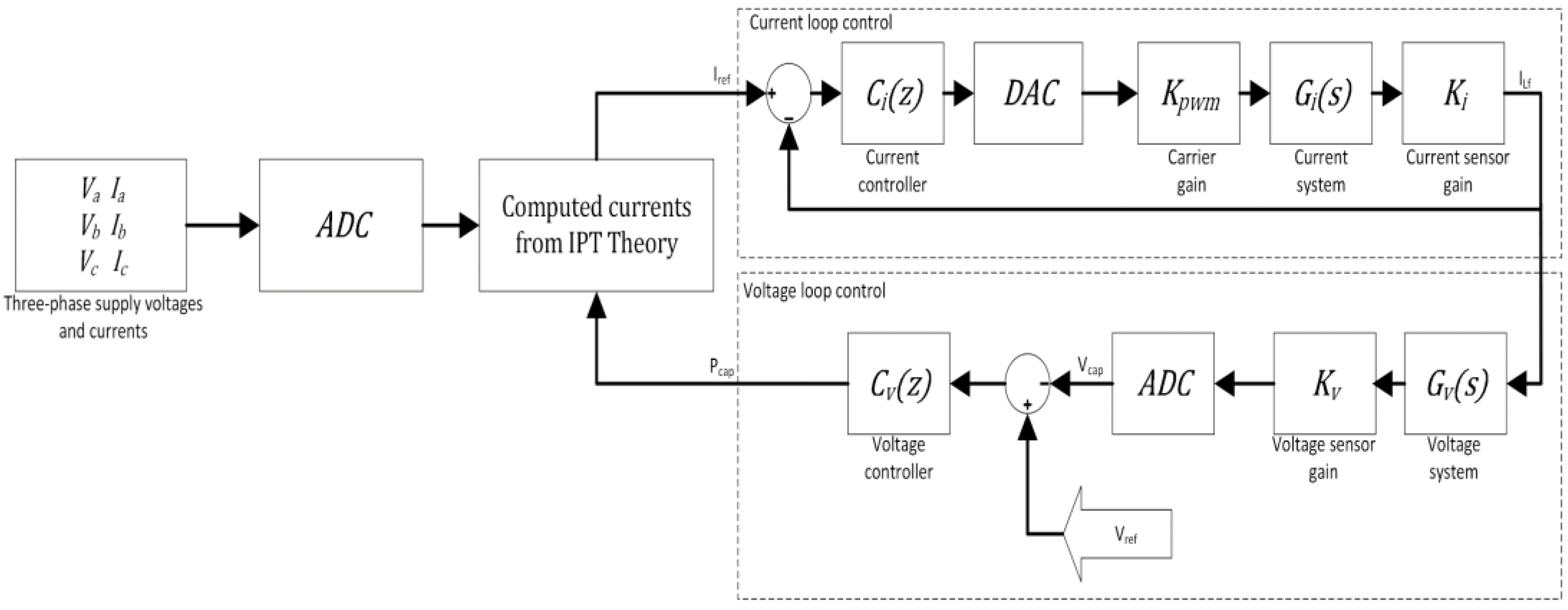
Figure 4 shows a flowchart to illustrate the steps for programming the power theories with the FIL technique. The ADC represents the conversion from the simulator to the board, and the DAC represents the simulator receiving the signals. The calculus are based on the equations of Section 3 and Table 4.

5. Simulation Results
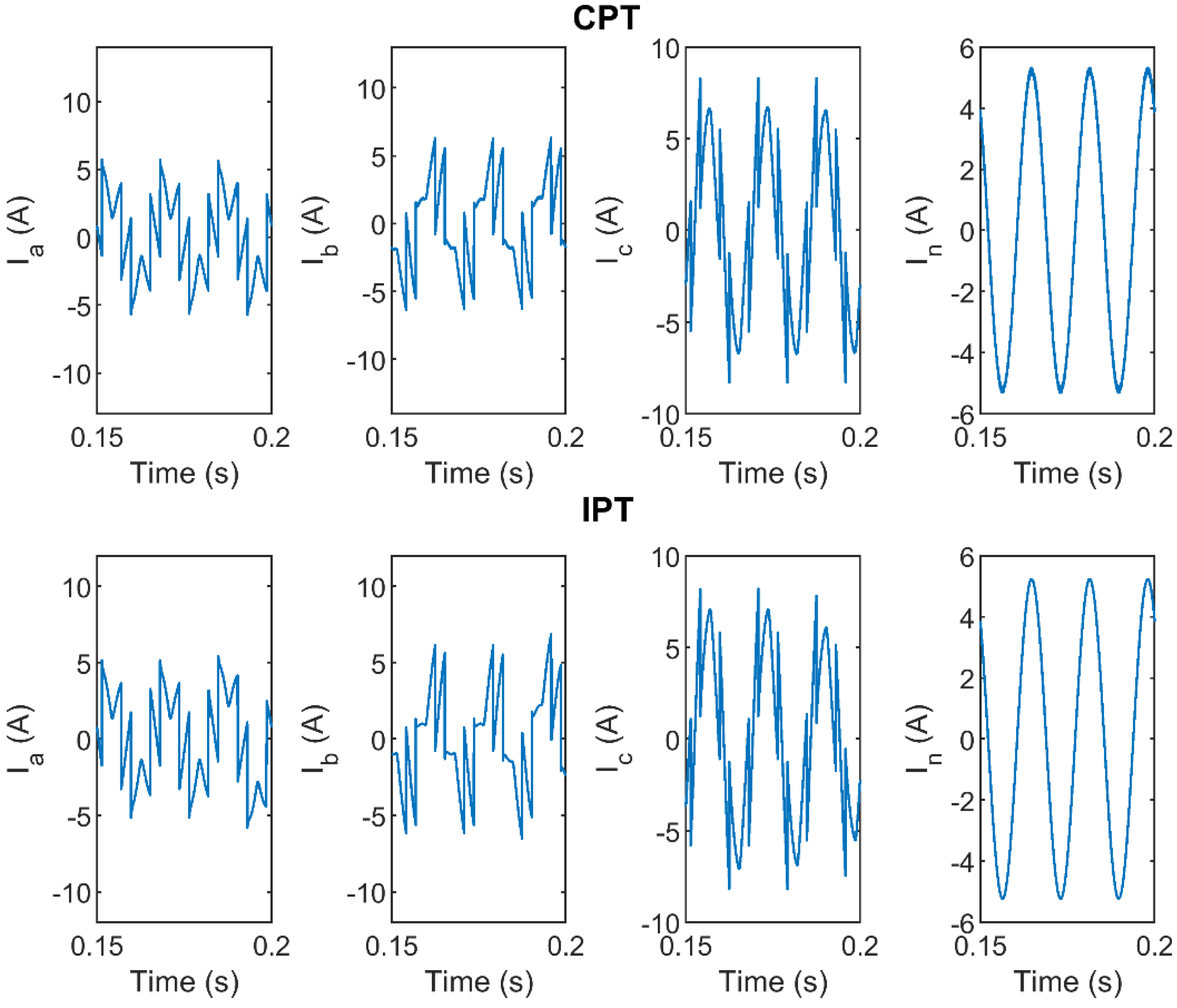
In Figure 5, it is possible to observe the compensation currents for each phase and the neutral of both theories responsible for providing the reference to the APPF.
For the selected loads, it appears that the compensation currents are quite similar. This result demonstrates that for certain cases of compensation, the two theories coincide in their formulation.
For the system operating with FIL, in Figure 6 and 
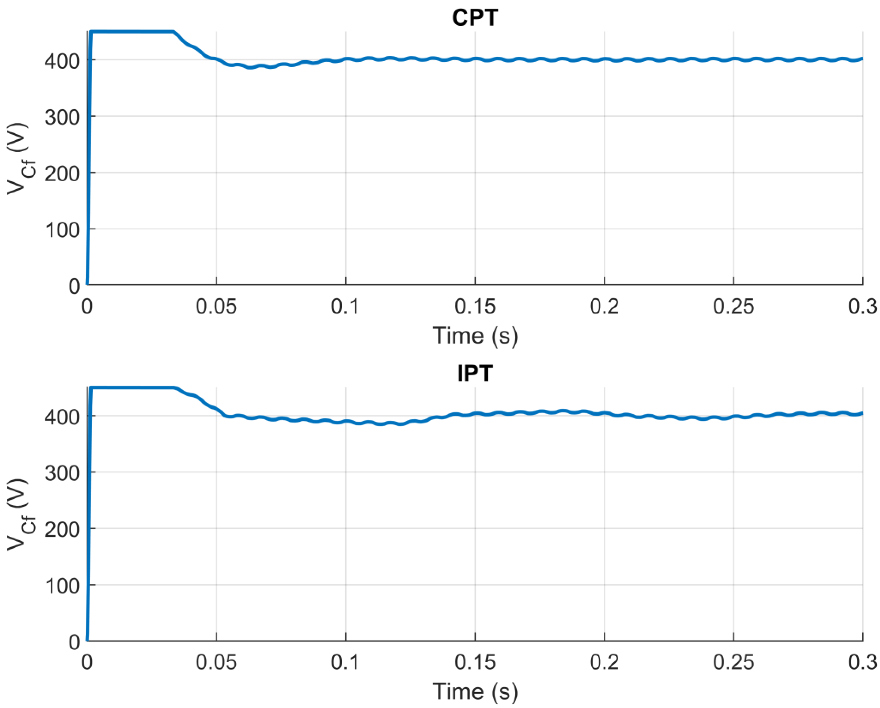
Figure 7, respectively, the source currents and the voltage in the APPF capacitance for both theories are observed.
The source currents can be analyzed in three distinct periods. In the first, not considered in this work, the capacitance Cf is charged. In the second, the unbalanced currents and the presence of harmonics are observed. In the third period, both controllers are started and the APPF starts to operate.
As can be seen, as soon as the compensation starts, the CPT presents a greater transient in the currents. This transient is a consequence of the multiple integral calculus and RMS values necessary to calculate the compensation currents. However, after the end of the transitory period, the compensation is as effective as in the IPT, leading the source to feed the system with a power factor (PF) of 0.9988.
Right at the beginning of the APPF operation, there is a relevant behavior to consider. The action of compensation causes sudden changes in the currents, leading to high derivatives that are not instantly absorbed by the circuit. Therefore, a transitory period is necessary until the stabilization of the currents according to the generated references.
As for the capacitance voltage, it is noticed that its dynamics in the CPT are faster than in the IPT even though its crossing-over frequency is higher than in the CPT. This is due to the quantities that are used in the voltage loop in each of the theories. In both theories, the voltage controller receives the difference between the 400 V reference and the capacitor voltage. However, the controller at the IPT sends a power signal that is added to the theory’s calculations and then transformed into current signals. In the CPT, the controller output is already given in a current format and is added directly to the compensation currents. Furthermore, it is observed that due to the voltage transient in the IPT, its current transient is also affected, and it is slower than that noticed in TPC. Additionally, the CPT provided a less oscillatory power as observed in Figure 7.
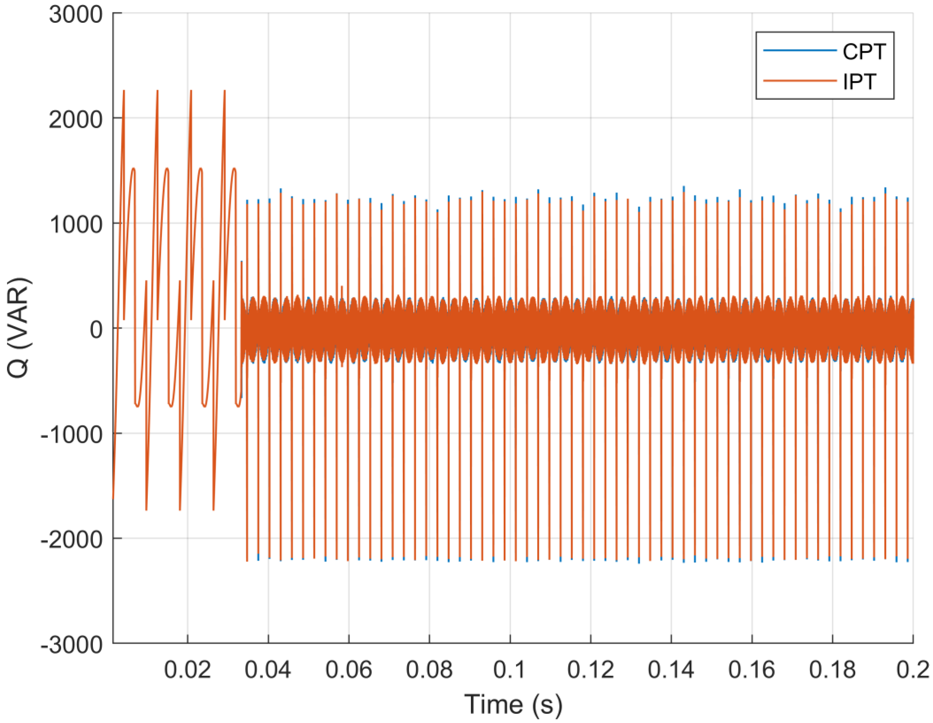
Because the reached PF is basically unitary, it is evident that the grid currents do not remain with some lag due to the presence of harmonics or uncompensated reactive energy. From Figure 8 and Figure 9, in which, respectively, the active and reactive powers supplied from the grid are presented, it is confirmed that in average terms, the entire reactive portion has been compensated.
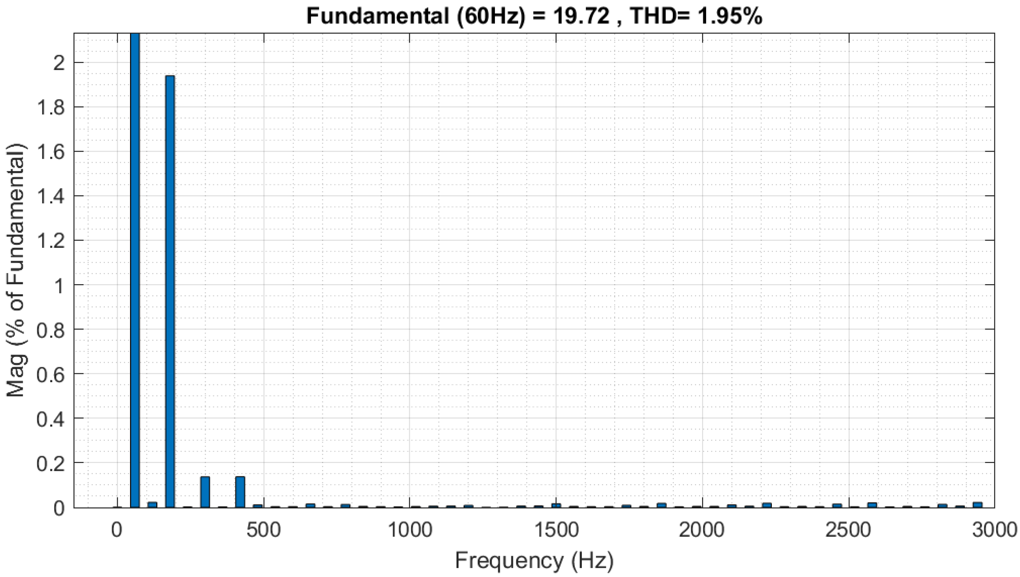
By analyzing the Total Harmonic Distortion (THD), it is possible to observe how the harmonics were treated in the system. Table 5 presents the data regarding the THD for the grid phases before and after the insertion of the APPF in the system.
According to the results, one can verify that the THD is considerably reduced compared to the system without APPF correction, resulting in 1.9% and 2.1%, when CPT is in operation, and in less than 1% when IPT is in operation. In Figure 10, the harmonic content up to the fiftieth order of phase “a” is presented for the APPF running with the CPT. This behavior is similar for the remaining phases and for the IPT theory.
It is also important to verify the compensation effectiveness by observing the individual harmonics as shown in Table 6. Table 6 shows the individual harmonics up to the 13th. For higher orders, all verified values are lower than 0.03%. As can be seen, the CPT has a higher harmonic content than the IPT, considering the load scenario in Table 2. However, its harmonic content is distributed among the 3rd, 5th, and 7th harmonics. As in the IPT, this content is relevant until the 13th.
Another behavior that should be highlighted is the greater impact of the third harmonic (180 Hz). For the case analyzed in Figure 10, this harmonic corresponds to about 1.94% of the fundamental. This frequency inserted into the current is associated with the capacitor voltage control. Its power is provided by the operation as a three-phase rectifier, which, in turn, ends up generating current harmonics with triple the fundamental frequency.
Eventually, one can conclude why the harmonics of the CPT and the IPT are slightly different. Basically, it is a direct consequence of the voltage outer loop in each theory. Depending on the tuning, the outer loop dynamic can be somewhat significant on the current and the resulting THD.
In order to compare the compensation effectiveness of the present work, we have chosen two works from the current literature. The work in [29] shows the effectiveness of an APPF regarding current compensation using a Genetic Algorithm and a Queen-Bee assisted Genetic Algorithm to optimize the controller coefficients. In [30], the current control is performed through a model predictive control. The strategy has as its purpose balance between THD, to maintain its level below IEEE standards and the value of the switching frequency. Therefore, they used a variable switching frequency around the base value shown in Table 7.
It is worth mentioning that in both works, resistances and inductances are used in the power source and at the point of connection of the loads, representing the cables impedance. Another important fact is the usage of an initial voltage in the DC bus capacitor. In [29] it is assumed as 200 V, whereas in [30], it is assumed as 100 V. In both cases, these assumptions facilitate the compensation of the APPF reducing the current peaks and settling time. Regarding the impedance, it helps the compensation currents to flow exclusively to the load. However, it is important to emphasize that in this work, the used initial capacitor voltage nor additional impedances are used.
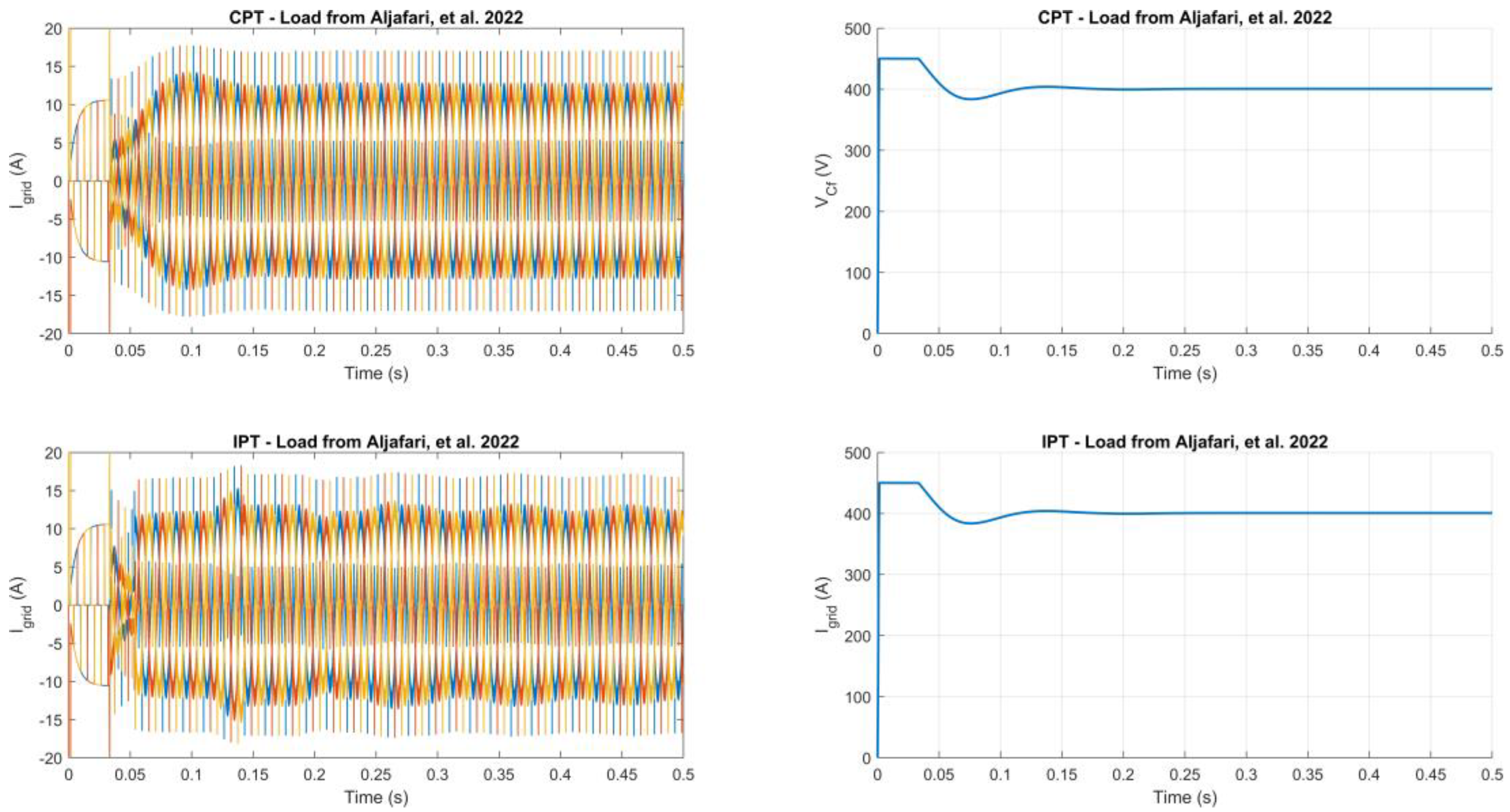
For the comparison scenario, the grid and the power electronics converter were the same, but the loads were changed to comply with the aforementioned references. A full-wave rectifier feeds the RL loads, and these data are shown in Table 7. Figure 11 and Figure 12 show the current and voltage waveforms at the power source for both load situations of [29,30]. Table 8 compares the THD of the current for each phase with the two mentioned controls.
Furthermore, the results of the settling time for each case are also analyzed. Observing the work of [29], the obtained settling time was 0.23 s and for [30], there is no available data.
Regarding the application of the PI controllers in IPT and CPT, ignoring the charging time of the capacitor, which is negligible, and knowing that the control starts to operate after two grid cycles, in t = 0.033 s, the settling time for IPT with loads of [29,30] are, respectively, t = 0.17 s and t = 0.10 s. As for the CPT, they are t = 0.12 s and t = 0.10 s. The steady-state regime was considered when the values were within ± 2 % .

6. Conclusions

The operation of parallel processes and the high processing speed of the FPGA are significant differentials for implementing APPF with a high switching frequency. Furthermore, the usage of the simulator and the FPGA board establishing the FIL operation to validate the control and the necessary calculations proved to be a powerful prototyping tool. Such technology allowed for the comparison between the two compensation strategies, with different methods for the reference currents generation with embedded controllers without the necessity for the physical topology for validations and without changing hardware for digital implementation.
Both theories proved valid for the APPF operation, hardware synthesis, and FPGA-in-the-loop implementation. However, since the CPT presents a more complex calculus with more processes than the IPT, a great processing requirement was identified in the usage of logic elements and blocks dedicated to the multiplication on the FPGA board. As a result, the implementation of each theory must be evaluated given the needs of the project and the available computational resources. If the compensation necessity is only related to the reactive power and the available resources are of worry one may use the IPT. If the computational resource is not an important point and different portions of power are necessary to be known or compensated, the CPT is the ideal theory to be implemented.
It is noteworthy that the FIL validation technique opens doors for comparing the performance of different linear and non-linear controllers for the implementation of APPF. In addition, other topologies and control techniques for active power filters can be analyzed to reduce the consequences of their insertion into the system through the FIL implementation. Finally, it is important to verify the quality of the achieved compensation with very low remaining distortion using the FPGA in comparison to other proposals. This is related to the high switching frequency of the used APPF allowed by the high processing power of the FPGA board.

Author Contributions

Conceptualization and methodology, N.D.d.A. and R.B.G.; validation, N.D.d.A., R.B.G. and R.L.R.S.; formal analysis, R.B.G., E.A.B. and M.A.G.d.B.; investigation, N.D.d.A. and R.L.R.S.; resources, N.D.d.A., M.A.G.d.B. and R.L.R.S.; writing—original draft preparation, N.D.d.A.; writing—review and editing, M.A.G.d.B. and E.A.B.; supervision, R.B.G.; project administration, R.B.G.; funding acquisition, E.A.B. All authors have read and agreed to the published version of the manuscript.

Funding

This study was financed in part by the Coordenação de Aperfeiçoamento de Pessoal de Nível Superior—Brasil (CAPES)—Finance Code 001 and the Research and Development Project—P&D ANEEL. PD-06961-0010/2019.

Institutional Review Board Statement

Not applicable.

Informed Consent Statement

Not applicable.

Data Availability Statement

Not applicable.

Acknowledgments

The authors want to thank the Federal University of Mato Grosso do Sul—UFMS.

Conflicts of Interest

The authors declare no conflict of interest.

References

  1. Bao, G.; Ke, S. Load Transfer Device for Solving a Three-Phase Unbalance Problem under a Low-Voltage Distribution Network. Energies 2019, 12, 2842. [Google Scholar] [CrossRef]
  2. Pires, V.F.; Cordeiro, A.; Foito, D.; Pires, A.J.; Hao, C.; Martins, J.F.; Castro, R. Compensation of Unbalanced Low-Voltage Grids Using a Photovoltaic Generation System with a Dual Four-Leg, Two-Level Inverter. Electronics 2022, 11, 320. [Google Scholar] [CrossRef]
  3. Graña-López, M.A.; García-Diez, A.; Filgueira-Vizoso, A.; Chouza-Gestoso, J.; Masdías-Bonome, A. Study of the Sustainability of Electrical Power Systems: Analysis of the Causes that Generate Reactive Power. Sustainability 2019, 11, 7202. [Google Scholar] [CrossRef]
  4. Montoya, O.; Alarcon-Villamil, J.; Hernández, J. Operating Cost Reduction in Distribution Networks Based on the Optimal Phase-Swapping including the Costs of the Working Groups and Energy Losses. Energies 2021, 14, 4535. [Google Scholar] [CrossRef]
  5. Grasel, B.; Baptista, J.; Tragner, M. Supraharmonic and Harmonic Emissions of a Bi-Directional V2G Electric Vehicle Charging Station and Their Impact to the Grid Impedance. Energies 2022, 15, 2920. [Google Scholar] [CrossRef]
  6. Satish, R.; Vaisakh, K.; Abdelaziz, A.Y.; El-Shahat, A. A Novel Three-Phase Harmonic Power Flow Algorithm for Unbalanced Radial Distribution Networks with the Presence of D-STATCOM Devices. Electronics 2021, 10, 2663. [Google Scholar] [CrossRef]
  7. Mohamed, M.; Ali, Z.; Ahmed, M.; Al-Gahtani, S. Energy Saving Maximization of Balanced and Unbalanced Distribution Power Systems via Network Reconfiguration and Optimum Capacitor Allocation Using a Hybrid Metaheuristic Algorithm. Energies 2021, 14, 3205. [Google Scholar] [CrossRef]
  8. Xu, S.; Wang, Y.; Xiao, X.; Xu, W.; Wang, Y. Adaptive Damping—An Improved Resonance Mitigation Scheme for Shunt Capacitors. IEEE Trans. Power Deliv. 2022, 37, 755–764. [Google Scholar] [CrossRef]
  9. Buła, D.; Grabowski, D.; Maciążek, M. A Review on Optimization of Active Power Filter Placement and Sizing Methods. Energies 2022, 15, 1175. [Google Scholar] [CrossRef]
  10. Lumbreras, D.; Gálvez, E.; Collado, A.; Zaragoza, J. Trends in Power Quality, Harmonic Mitigation and Standards for Light and Heavy Industries: A Review. Energies 2020, 13, 5792. [Google Scholar] [CrossRef]
  11. Akagi, H.; Watanabe, E.H.; Aredes, M. Instantaneous Power Theory and Applications to Power Conditioning. In SciTech Book News; John Wiley & Sons: Hoboken, NJ, USA, 2007; Volume 31. [Google Scholar]
  12. Tenti, P.; Paredes, H.K.M.; Mattavelli, P. Conservative Power Theory, a Framework to Approach Control and Accountability Issues in Smart Microgrids. IEEE Trans. Power Electron. 2010, 26, 664–673. [Google Scholar] [CrossRef]
  13. Queiroz, J.; Carvalho, S.; Barros, C.; Barros, L.; Barbosa, D. Embedding an Electrical System Real-Time Simulator with Floating-Point Arithmetic in a Field Programmable Gate Array. Energies 2021, 14, 8404. [Google Scholar] [CrossRef]
  14. Sankar, D.; Syamala, L.; Ayyappan, B.C.; Kallarackal, M. FPGA-Based Cost-Effective and Resource Optimized Solution of Predictive Direct Current Control for Power Converters. Energies 2021, 14, 7669. [Google Scholar] [CrossRef]
  15. Cirugeda-Roldán, E.M.; Martínez-García, M.S.; Sanchez, A.; de Castro, A. Evaluation of the Different Numerical Formats for HIL Models of Power Converters after the Adoption of VHDL-2008 by Xilinx. Electronics 2021, 10, 1952. [Google Scholar] [CrossRef]
  16. Garrido, M.J.; Pescador, F.; Chavarrias, M.; Lobo, P.J.; Sanz, C. A High Performance FPGA-Based Architecture for the Future Video Coding Adaptive Multiple Core Transform. IEEE Trans. Consum. Electron. 2018, 64, 53–60. [Google Scholar] [CrossRef]
  17. Urbina, M.; Moreira, N.; Rodriguez, M.; Acosta, T.; Lázaro, J.; Astarloa, A. Secure Protocol and IP Core for Configuration of Networking Hardware IPs in the Smart Grid. Energies 2018, 11, 510. [Google Scholar] [CrossRef]
  18. Valente, G.; Muttillo, V.; Muttillo, M.; Barile, G.; Leoni, A.; Tiberti, W.; Pomante, L. SPOF—Slave Powerlink on FPGA for Smart Sensors and Actuators Interfacing for Industry 4.0 Applications. Energies 2019, 12, 1633. [Google Scholar] [CrossRef]
  19. Xing, Y.; Liang, S.; Sui, L.; Jia, X.; Qiu, J.; Liu, X.; Wang, Y.; Shan, Y.; Wang, Y. DNNVM: End-to-End Compiler Leveraging Heterogeneous Optimizations on FPGA-Based CNN Accelerators. IEEE Trans. Comput. Des. Integr. Circuits Syst. 2019, 39, 2668–2681. [Google Scholar] [CrossRef]
  20. Dai, X.; Ke, C.; Quan, Q.; Cai, K.-Y. Simulation Credibility Assessment Methodology with FPGA-based Hardware-in-the-Loop Platform. IEEE Trans. Ind. Electron. 2020, 68, 3282–3291. [Google Scholar] [CrossRef]
  21. Infineon Technologies: Semicondutor & System Solutions. Silicon Carbide MOSFET Discretes. Available online: https://www.infineon.com/cms/en/product/power/mosfet/silicon-carbide/discretes/imw65r107m1h/ (accessed on 5 August 2022).
  22. Erickson, R.W.; Makisomovic, D. Fundamentals of Power Electronics, 3rd ed.; Springer: Berlin/Heidelberg, Germany, 2020; p. 1081. [Google Scholar]
  23. Ma, J.; Wang, X.; Blaabjerg, F.; Harnefors, L.; Song, W. Accuracy Analysis of the Zero-Order Hold Model for Digital Pulse Width Modulation. IEEE Trans. Power Electron. 2018, 33, 10826–10834. [Google Scholar] [CrossRef] [Green Version]
  24. Ogata, K. Discrete-Time Control Systems, 2nd ed.; Pearson: London, UK, 2000; p. 768. [Google Scholar]
  25. Eskandarian, N.; Beromi, Y.A.; Farhangi, S. Improvement of Dynamic Behavior of Shunt Active Power Filter Using Fuzzy Instantaneous Power Theory. J. Power Electron. 2014, 14, 1303–1313. [Google Scholar] [CrossRef]
  26. Depenbrock, M.; Staudt, V.; Wrede, H. A theoretical investigation of original and modified instantaneous power theory applied to four-wire systems. IEEE Trans. Ind. Appl. 2003, 39, 1160–1168. [Google Scholar] [CrossRef]
  27. Burgos-Mellado, C.; Cardenas, R.; Saez, D.; Costabeber, A.; Sumner, M. A Control Algorithm Based on the Conservative Power Theory for Cooperative Sharing of Imbalances in Four-Wire Systems. IEEE Trans. Power Electron. 2018, 34, 5325–5339. [Google Scholar] [CrossRef]
  28. Mota, D.; Tedeschi, E. On Adaptive Moving Average Algorithms for the Application of the Conservative Power Theory in Systems with Variable Frequency. Energies 2021, 14, 1201. [Google Scholar] [CrossRef]
  29. Sundaram, E.; Gunasekaran, M.; Krishnan, R.; Padmanaban, S.; Chenniappan, S.; Ertas, A.H. Genetic algorithm-based reference current control extraction-based shunt active power filter. Int. Trans. Electr. Energy Syst. 2020, 31, e12623. [Google Scholar] [CrossRef]
  30. Aljafari, B.; Rameshkumar, K.; Indragandhi, V.; Ramachandran, S. A Novel Single-Phase Shunt Active Power Filter with a Cost Function Based Model Predictive Current Control Technique. Energies 2022, 15, 4531. [Google Scholar] [CrossRef]
Figure 1. FIL scheme for the four-wire APPF simulation.
Energies 15 06284 g001
Figure 2. IPT control loops.
Energies 15 06284 g002
Figure 3. CPT control loops.
Energies 15 06284 g003
Figure 4. Flowchart to implementing FIL with IPT and CPT theories.
Energies 15 06284 g004
Figure 5. Power theory compensated currents obtained by FIL.
Energies 15 06284 g005
Figure 6. Comparison of the grid currents through FIL for the power theories. Phases (a), (b), (c) and neutral are in blue, red, yellow, and purple, respectively.
Energies 15 06284 g006
Figure 7. Comparison of Cf voltage using FIL for the power theories.
Energies 15 06284 g007
Figure 8. Grid supplied active power with APPF operating.
Energies 15 06284 g008
Figure 9. Grid supplied reactive power with APPF operating.
Energies 15 06284 g009
Figure 10. Phase “a” total harmonic distortion with APPF.
Energies 15 06284 g010
Figure 11. Comparison between CPT and IPT for the loads used in [29].
Energies 15 06284 g011
Figure 12. Comparison between CPT and IPT for the loads used in [30].
Energies 15 06284 g012
Table 1. Control parameters and system components.
ParametersValues
Switching frequency—fs400 kHz
Filter inductance—Lf_μ62.5 μH
DC bus capacitance—Cf1.8 mF
Filter resistance—Rf2.4 mΩ
DC bus voltage—VCC400 V
Electrical system line voltage—VLRMS220 V
Maximum current ripple—Δimáx2 A
Table 2. Loads supplied by the system.
LoadsPhase aPhase bPhase c
Linear—RL1 kW; 0.1 kVAr0.9 kW; 0.09 kVAr0.5 kW; 0.11 kVAR
Rectifier—RL10 mH; 40 Ω10 mH; 40 Ω10 mH; 40 Ω
Linear—R80 Ω80 Ω-
Table 3. Gains of analog (K) and digital (g) controllers.
ParametersCi(s); Ci(z) (IPT)Cv(s); Cv(z) (IPT)Ci(s); Ci(z) (CPT)Cv(s); Cv(z) (CPT)
Kp0.4257750.70.425757.88
Ki5.35 × 104 6.132 × 1055.35 × 1043637
gx10.42574634733750.6760244140.4257463473357.879697639
gx2−0.3722454834−750.062866166−0.3722454834−57.876060950
Table 4. Computational resources need for each theory.
Implemented Power TheoryIPTCPT
Logical elements7.839/114.480 (7%)54.833/114.480 (48%)
Registers 4631377
IOs483/529 (91%)483/529 (91%)
Memory bits0/3.981.312 (0%)0/3.981.312 (0%)
9 bits embedded multipliers180/532 (34%)461/532 (87%)
PLLs0/4 (0%)0/4 (0%)
Table 5. System total harmonic distortion.
THDPhase aPhase bPhase c
Without APPF10.79%11.24%17.72%
APPF—CPT1.95%2.05%1.99%
APPF—IPT0.80%0.81%0.81%
Table 6. Individual harmonics up to the 13th.
CPT IPT
OrderFrequencyPhase aPhase bPhase cPhase aPhase bPhase c
2nd1200.020.030.030.210.390.40
3rd1801.951.991.960.820.740.86
4th2400.000.010.010.050.160.16
5th3000.140.150.140.120.160.24
6th3600.000.010.010.020.090.09
7th4200.140.140.140.120.150.18
8th4800.010.010.020.020.060.06
9th5400.000.000.000.010.060.06
10th6000.000.010.010.010.050.05
11th6600.020.020.020.060.090.05
12th7200.000.000.000.010.050.05
13th7800.010.010.010.050.080.05
Table 7. Load parameters for comparison purposes.
Parameters[29][30]
LoadsLL = 40 mH; RL = 50 ΩLL = 160 mH; RL = 28 Ω
Grid frequency and voltage fg = 50 Hz; Vg = 140 Vfg = 50 Hz; Vg = 100 V
DC linkCf = 3300 µF; VDC = 300 VCf = 100 µF; VDC = 200V
Switching frequencyfs = 15 kHz (base)fs = 20 kHz
Table 8. THD of the supply current in %.
Phase aPhase bPhase c
Control/Power TheoryWorkbenchWithout APPFWith APPFWithout APPFWith APPFWithout APPFWith APPF
PI/IPT (Load [29])FIL29.450.7029.451.0629.450.96
PI/CPT (Load [29])FIL29.450.2829.450.2729.450.28
PI/IPT (Load [30])FIL34.200.4534.200.5134.200.58
PI/CPT (Load [30])FIL34.200.2534.200.2534.200.25
GA [29]Simulation22.633.1522.633.1522.633.15
GA [29]Hardware22.633.7122.633.9422.633.18
QBGA [29]Simulation22.631.9622.631.9622.631.96
QBGA [29]Hardware22.633.5022.633.1222.633.01
MPC [30]Simulation28.47 3.53 1∅
MPC [30]Hardware24.90 3.70 1∅
Publisher’s Note: MDPI stays neutral with regard to jurisdictional claims in published maps and institutional affiliations.

