Machine Learning Approach for Short-Term Load Forecasting Using Deep Neural Network

Abstract

Power system demand forecasting is a crucial task in the power system engineering field. This is due to the fact that most system planning and operation activities basically rely on proper forecasting models. Entire power infrastructures are built essentially to provide and serve the consumption of energy. Therefore, it is very necessary to construct robust and efficient predictive models in order to provide accurate load forecasting. In this paper, three techniques are utilized for short-term load forecasting. These techniques are deep neural network (DNN), multilayer perceptron-based artificial neural network (ANN), and decision tree-based prediction (DR). New predictive variables are included to enhance the overall forecasting and handle the difficulties caused by some categorical predictors. The comparison among these three techniques is executed based on coefficients of determination R² and mean absolute error (MAE). Statistical tests are performed in order to verify the results and examine whether these models are statistically different or not. The results reveal that the DNN model outperformed the other models and was statistically different from them.

1. Introduction

Load forecasting is a significant component of distribution-system planning and operation [1]. By means of predictive models, the pattern of the demand is being investigated, and some electrical generators are assigned to meet this demand at subtransmission and distribution networks, so any large deviation in the forecasting could cause technical and economical problems [2]. Furthermore, in deregulated power system marketing, all the bidding strategies from both the energy producer and the customer are directly dependent on the forecast demand [2]. Frequently, there is a delay between awareness of an increase in load demand and the occurrence of that increase. This time allows electrical engineers to perform the task of planning and forecasting to meet the expected demand increase. A load forecast is required in order to determine when an increase on load will occur so that suitable actions can be taken.

The required forecast horizon determines the type of forecasting, whether it is long, medium, or short term. In short-term forecasting, the time span is intended to be 1 h ahead up to 1 week, including daily forecasting (24 h). Many operation activities are done in this short period, such as generator dispatching, unit commitment, voltage regulating, real-time pricing in the energy market, and more. As such, accurate short-term load forecasting methods require data that are mainly associated with the time dimension: historical load, historical weather conditions, predicted weather conditions, and the nature of the day and the season are examples of the required data for the short-term electric load forecast. The following are the generalized important factors for proper load forecast studies [3]:

• Historical load data in megawatts (MW) and megavolt amperes (MAVR).
• Weather conditions (temperature, dew point, pressure, sky cover, visibility, wind speed, etc.).
• Economic indicators (energy prices, local industrial production, housing starts, etc.).
• Time factor (time of the year, the day of the week, and hour of the day).
• Customers’ classes (residential, commercial, industrial, hospitals, etc.).

Time factors and weather conditions besides the historical load demand should be handled carefully in electric load forecast studies. The time factor takes into account different scales, such as the months in a year, days in a week, and hours in a day. Also, an index can be utilized in load forecasting studies that distinguish between weekdays and weekends. The second important factor in short-term power demand forecast is how the weather conditions affect the behavior of the load. Various weather variables are considered by different utilities and research engineers to capture the effect of weather conditions (temperature, wind, humidity) on electric load forecast. Utilities widely utilize two factors to capture these effects: the first factor is related to temperature and humidity indices and is usually utilized in summer to capture the effect of heat and humidity on electric consumption. Other indices that are related to wind speed, temperature, and rate of ice falling are utilized in winter. Customers’ classes play an essential role as well in order to define the pattern of the forecast load. Each individual dataset should be inspected manually. However, when there are large datasets to analyze, manually cleaning each data file individually will require substantial time and effort, and automated examination may be the best alternative, using some well-established statistically based methods.

A variety of methods, such as naïve approaches, simple regression analysis, time-series analysis, and methods based on soft computing, have been deployed for short electric load forecast [4,5,6,7,8,9,10,11,12,13,14,15,16,17,18,19,20,21,22,23]. Short-term load forecasting was presented using multiple linear regression incorporating polynomial terms in [4]. Papalexopoulos et al. [5] proposed a linear regression model incorporating heating and cooling functions, as well as binary variables. SA short-term load forecast is presented in reference [6] using the application of nonparametric regression inspired by the probability distribution function for the load and some affecting variables. Song et al. [7] employed a fuzzy regression analysis for short-term demand prediction that encompassed the effect of holidays on the predictive model. Load forecasting was employed by Heinemann et al. [8] using regression analysis, taking into account two components of loads: temperature-sensitive load and non-temperature-sensitive load. An adaptive short-term forecasting of hourly loads using multivariate regression was applied in [11]. Krogh et al. [12] combined regression with autoregression integrated moving average to provide an online load prediction. Artificial neural network (ANN) is used to forecast the electric demand in [13,14]: the only data involved in the model are temperature and load data. Short-term load forecasting is implemented utilizing cascaded learning methods parallel with load and temperature records [15], and this method is called cascaded artificial neural networks (CANNs). A fuzzy neural network is proposed for the short-term load forecast [16,17]. Chen et al. [18] used a non-fully connected ANN for short-term forecasting in order to minimize the training time. In [19], load pattern based on both weekdays and weekends was modeled. Active selection for training data, k-nearest neighbors, and pilot simulation are incorporated with ANN to forecast the short-term demand [20]. Ho et al. [21] designed a multilayer neural network with an adaptive learning algorithm for short-term load forecast. The authors in [22] used the decision tree ID3 to forecast the load in the long term, while the authors in [23] applied expert systems besides the ID3 decision tree to forecast the short-term demand.

To the best of our knowledge, this is the only work to compare two machine based learning techniques (ANN and DT) with a regression model. In addition, there is a lack in the literature of utilizing decision tree-based machine learning in short-term load forecasting, so this work focuses on that as well. Many published papers in the literature have not used statistical tests (parametric/nonparametric); hence, results cannot be verified without using statistical tests [24]. Therefore, this paper applies statistical tests in order to verify the results and examine whether the predictive model that has been used produces results that are statistically different or not.

This paper is organized into four sections: (1) introduction in Section 1, (2) Section 2 shows the datasets and methodology, which include the proposed approach, brief information of datasets for the experimental demonstration, data preparation and correlation analysis; methods for load forecasting (such as DNN, ANN, DT implementation), and model performance criteria, and (3) Section 3 presents the results and discussion for three different type of forecasting (per hour, per day, and per week), and (4) the conclusion is presented in Section 4.

2. Datasets and Methodology

The proposed approach is shown in Figure 1, which is a combination of 7 basic steps. These steps are: (1) online/offline dataset collection, (2) data preprocessing, (3) feature extraction, (4) most relevant feature selection, (5) AI model development, (6) forecast value extraction, and (7) result comparison. The collected dataset may be online or offline, which is selected as per the user’s application. After collecting the dataset, data preprocessing is performed to eliminate the spikes and fill missing values, if any. Generally, spikes and missing values in the dataset occur due to several issues/reasons, such as unwanted weather conditions and/or instrumental/operational/technical and human error. After preprocessing the dataset, feature extraction is performed, which includes several possible combinations of features, such as statistical features (mean, SD, variance, kurtosis, etc.), time-domain features, frequency-domain features, and time-frequency-domain features. Feature selection is performed to select the most relevant input variables/features that affect the performance of the AI/machine learning model for forecasting. Thereafter, forecasting model development is performed, which may include different types of models, such as linear time-series model (AR, MA, ARMA, ARIMA, ARFIMA, SARIMA, etc.), nonlinear time-series model (ARCH, GARCH, EGARCH, TAR, NAR, NMA, etc.), and AI/ML-based model (ANN, SVM, ELM, PSO, GA, ACO, decision tree, etc.). After the model development, training and testing are performed to validate the model performance, and finally obtained results are compared to obtain the best model for future forecasting applications. For more detail regarding demonstration of step-step-wise procedure of implementation of feature extraction and selection, the reader may refer [25,26,27,28,29,30,31] and [25,26,27,32,33,34], respectively.

Figure 1. Proposed approach for load forecasting.

2.1. Brief Information on Datasets for the Experimental Demonstration

Short-load forecasting mainly depends on the weather conditions and the previous historical data for the demand. Three datasets have been used in this paper. The first dataset, which is related to the historical recorded power demand, is obtained from Independent Electricity System Operator (IESO) [35]. These demand readings represent the power demand in Ontario province in Canada. The second dataset is related to the weather conditions which was obtained from Canadian Climate Data—Environment Canada [36]. Enormous recorded data, including temperature, dew-point temperature, humidity, and others, are obtained in dataset 2. The third dataset was acquired from Independent Electricity System Operator as well [35], and it contains the hourly Ontario energy prices (HOEP). Energy prices play a key role in influencing the load patterns [37]. Since the dataset for the demand is quite large, a random sample containing 200 hourly readings from dataset 1 is generated. Then, the other variables in the remaining datasets are mapped into this hourly sample. To illustrate, if hour 50 is selected randomly from dataset 1, then all the predictors’ variables in each dataset in hour 50 will be selected and mapped to this hour to represent the first reading in the new dataset and so on. As such, the new dataset that will be used in the analysis contains 200 readings randomly selected to be unbiased. This sample was selected randomly using PHStat package [38]. Because the model is about to forecast the load for a short period of time, the hourly power demand is selected to be the dependent variable (model’s output), while the other variables shown in Table 1 are independent variables (model’s inputs). All the variables are numeric. It is worth mentioning that the predictor PW (previous week load for the same time) implicitly includes whether this hour in weekdays or weekends. Therefore, it gave an advantage for the model to transfer the categorical predictors into numeric predictors, making the model easy to implement. 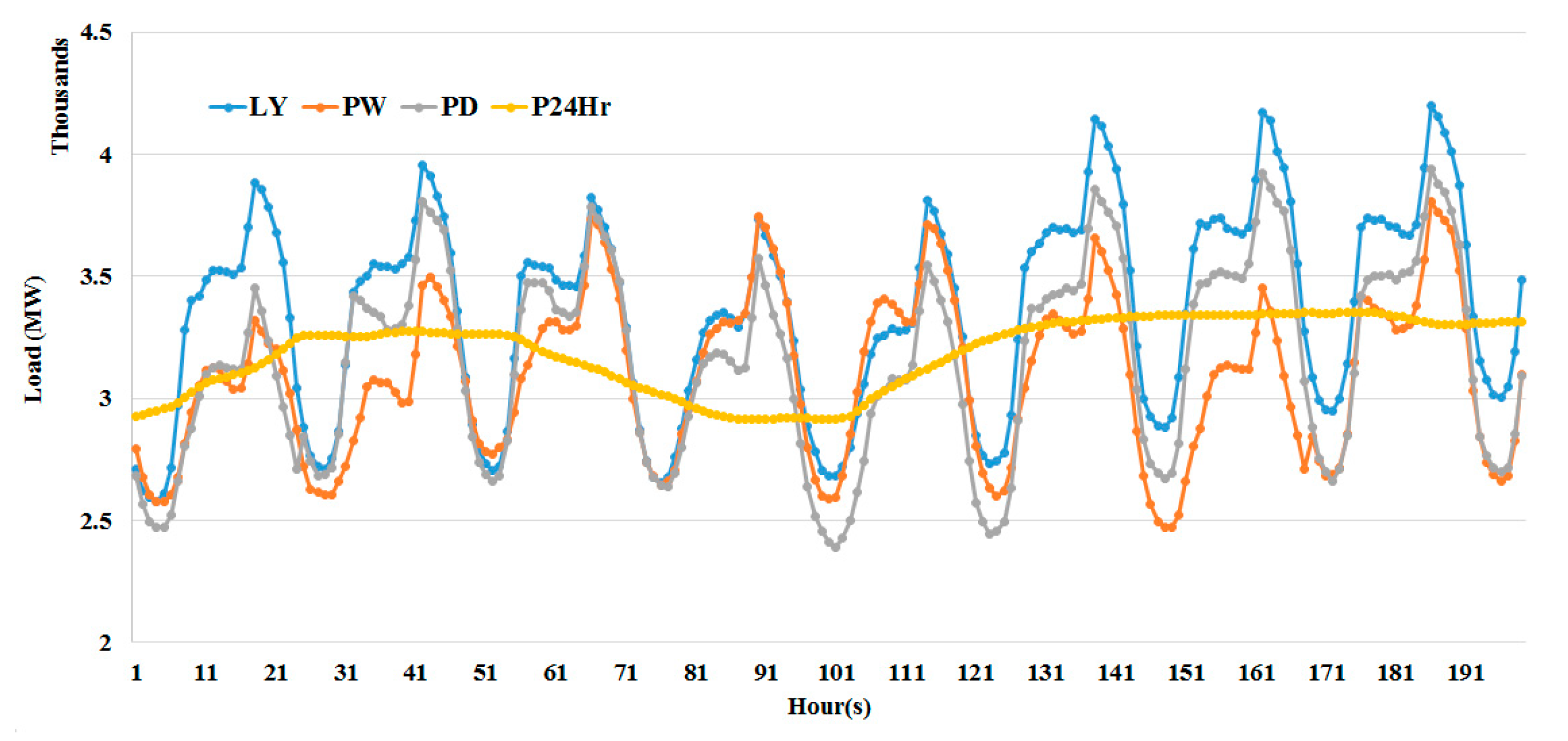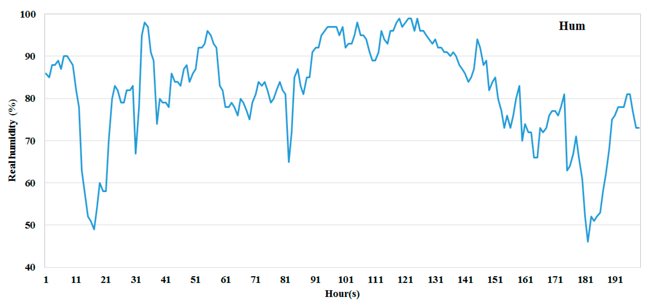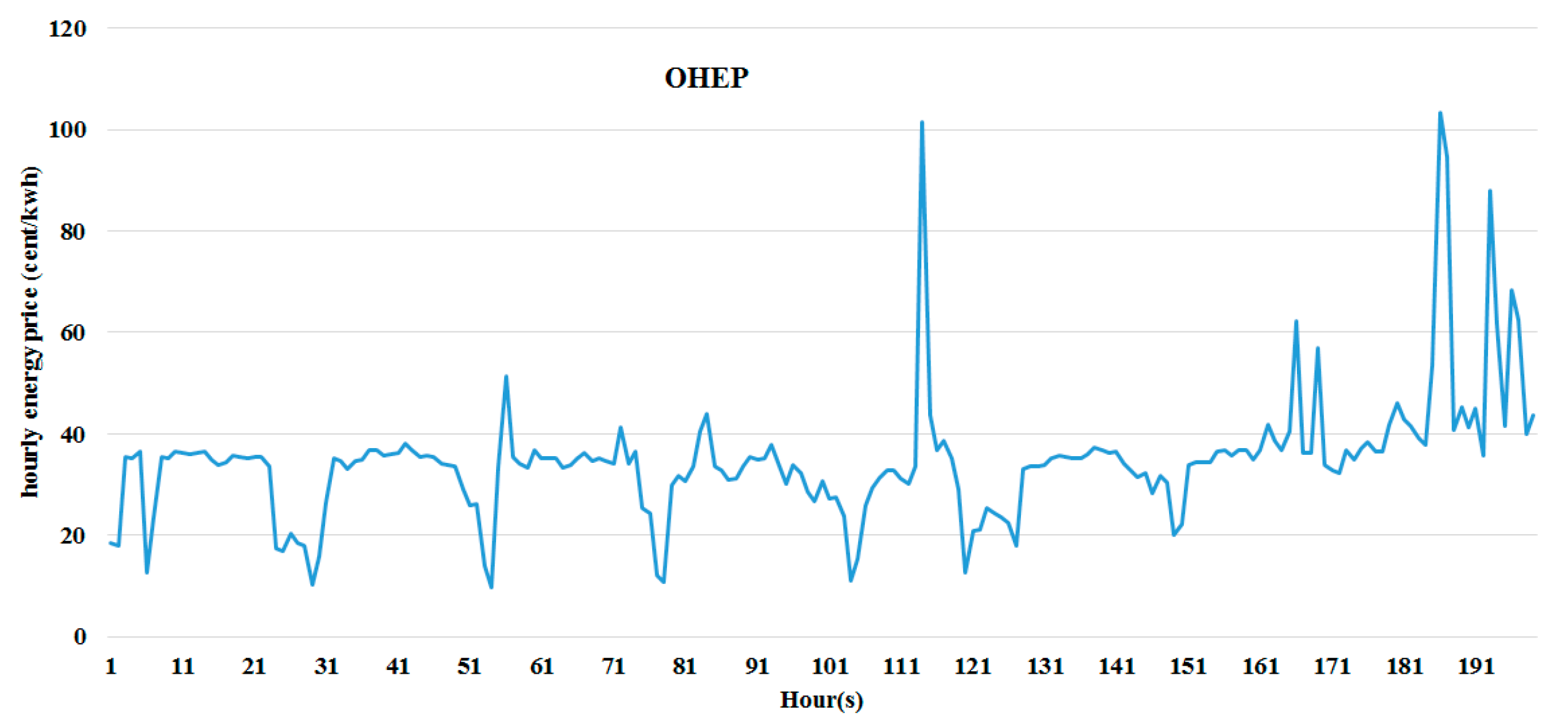Moreover, dataset characteristic is shown in Table 2 and are represented graphically in Figure 2, Figure 3, Figure 4, Figure 5, Figure 6 and Figure 7.

Table 1. Description of the dependent and independent variables.

Variable	Description—Type
Hourly Load	The estimated hourly load for the system (MW)
LY	Last year load at the same time (MW)
PW	Previous week load for the same time (MW)
PD	Previous day load for the same time (MW)
P24Hr	Average load for the 24 h prior to this time (MW)
Temp	Outside temperature (°C)
DT	Dew point temperature (°C)
Hum	Real humidity (%)
WS	Average wind speed (km/h)
AP	Outside air pressure (kPa)
OHEP	Ontario hourly energy price (cents/kwh)

Table 2. Dataset characteristics.

Variables	Statistical Information for Data
	Min	Mean	Max	STD
Hourly load	2387.356	3198.982	3937.756	396.3217
LY: Last year load at the same time (MW)	2574.196	3359.433	4197.332	408.688
PW: Previous week load for the same time (MW)	2473.032	3089.212	3807.772	329.1408
PD: Previous day load for the same time (MW)	2387.356	3151.728	3937.756	395.8146
P24Hr: Average load for the 24 h prior to this time (MW)	2912.799	3188.113	3351.651	149.6213
Temp: Outside temperature (°C)	5.8	13.40905	22.9	3.995968
DT: Dew point temperature (°C)	2.2	9.210553	15.9	4.57159
Hum: Real humidity (%)	46	81.96985	99	12.01837
WS: Average wind speed (km/h)	0	14.15578	35	6.852418
AP: Outside air pressure (kPa)	98.94	100.0777	101.34	0.568973
OHEP: Ontario hourly energy price (cent/kwh)	9.8	34.62302	103.39	12.51388

Figure 2. Load data information in MW.

Figure 3. Temperature data information (°C).

Figure 4. Humidity data information (%).

Figure 5. Wind speed data information (km/h).

Figure 6. Outside air pressure data information (kPa).

Figure 7. Hourly energy price data information (cents/kwh).

Data Preparation and Correlation Analysis

The data preparation procedure for the predictive models is common in most steps, especially in the preparation stage. The independent variables and dependent variables should be clearly distinguished. All data in this work are numeric. Then, the outliers are tested before applying any machine learning-based methods. Dixion’s Q test [39] is applied in order to identify the outliers in the dataset. In Dixion’ Q test, it is assumed that all data values come from the same normal population. The alternative hypothesis is that the smallest or largest values are outlier at a 5% significance level.

For multiple linear regression, stepwise regression is applied first in order to consider only the predictors that are statistically significant at 95% confidence. Descriptive analysis should be obtained, especially the coefficient of skewness (CS) and coefficient of kurtosis (CK). When CS is ranging between −0.5 and 0.5, this indicates that the data are relatively symmetric. The conditions of applying multiple linear regression should be tested before applying MLR, as stated previously. It has been found that the conditions to apply the MLR model, such as the normality of variables’ distribution and the linear relationship between the output variable and the predictors, are not met, so we used MLR with logarithmic transformation. Lastly, cross-validation with leave-one-out (LOO) was used in the model development. For machine learning methods, the models were trained and tested using the LOO technique. It is important to state that in machine learning techniques, all predictors were considered as inputs. This is because a predictor that was not considered significant in the regression model might be significant in machine learning-based models.

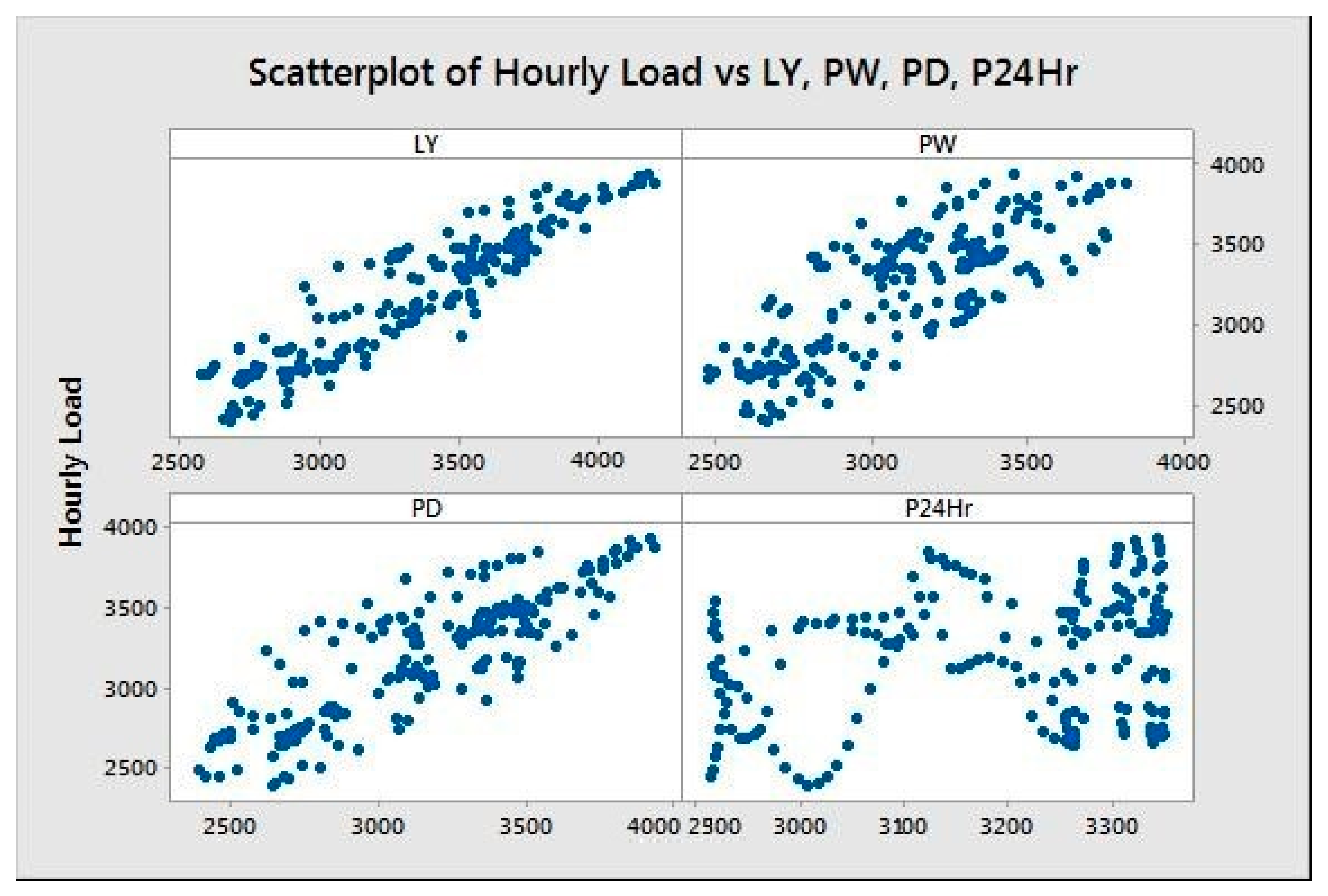
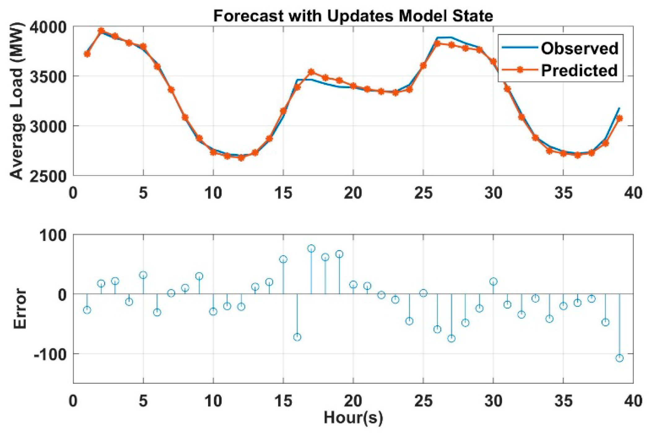
It is worth mentioning that the three models were trained/tested using the same datasets with LOO validation. This is to ensure that the comparison among these three models is fair and unbiased. Figure 8 shows the relationships between the hourly load and the independent variables LY, PW, PD, and P24Hr.

Figure 8. The relationships between the hourly load and the independent variables LY, PW, PD, and P24Hr.

2.2. Methods for Load Forecasting

Short-load forecast mainly depends on the weather conditions and the previous historical data for the demand. Three datasets have been used in this paper. The first dataset, which is related to the historical recorded power demand, is obtained from Independent Electricity System Operator (IESO) [35].

2.2.1. Deep Neural Network (DNN)

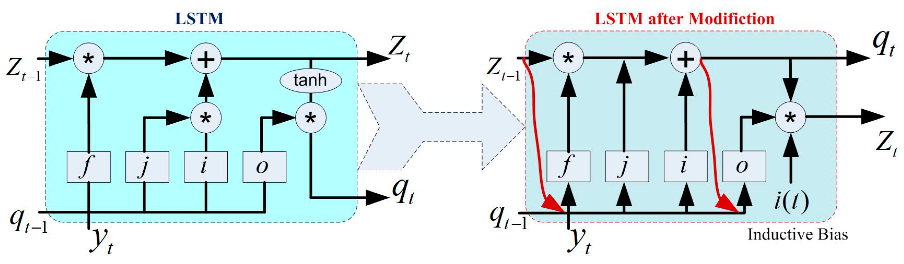
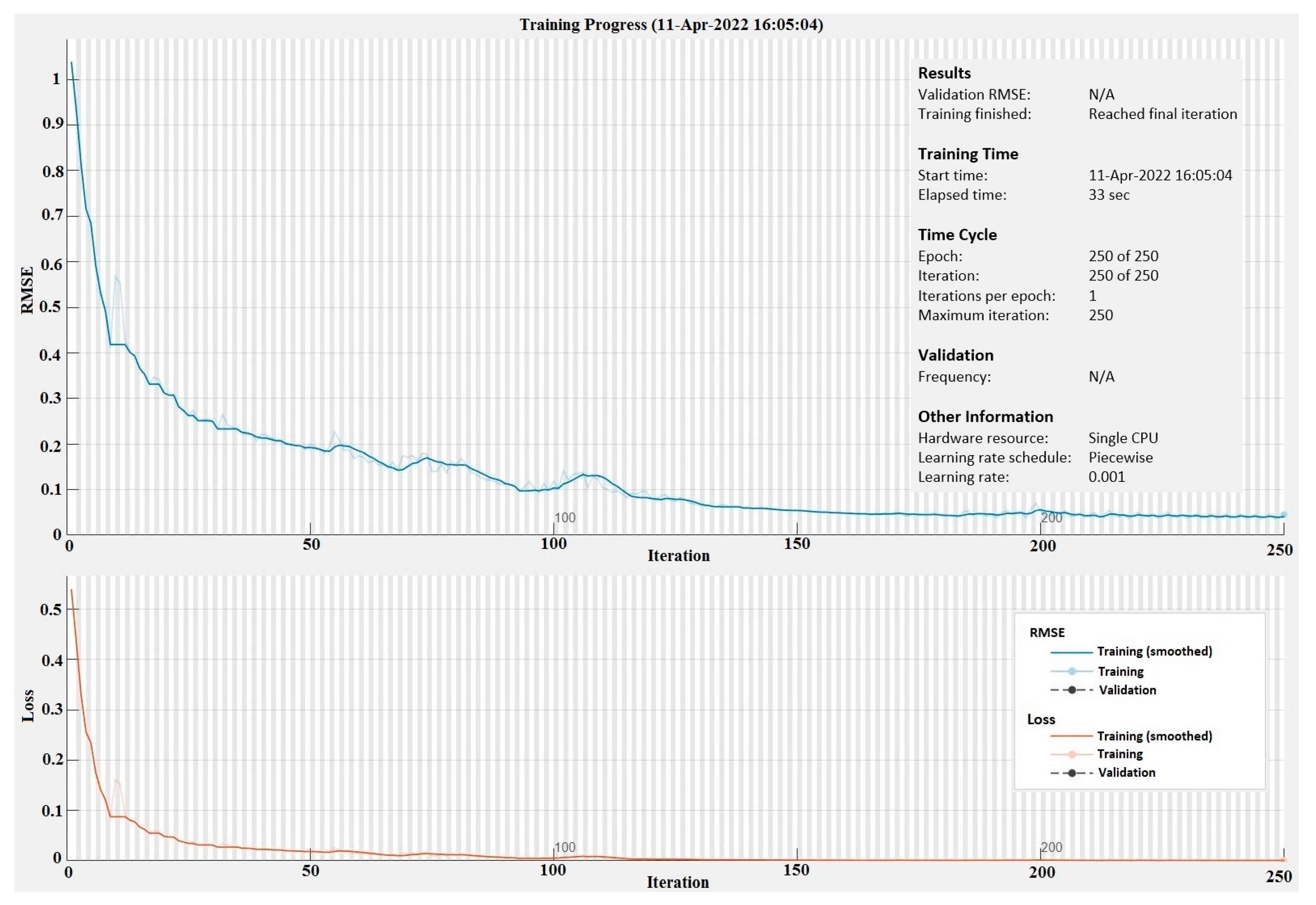
In the DNN, CNN is a type of ANN, which is the most implemented technique. But CNN is limited to the flow of parameter sharing and sequence data. After that, RNN is introduced to overcome these problems. At the same time, RNN has limited memory to store the operation of each stage and suffers from gradient problems [25,26,27], such as vanishing or exploding, etc. To resolve these problems, an advanced version of RNN was formulated, LSTM, in 1997 [32]. LSTM also works based on the sequential structure of 4 states. In this study, a modified LSTM is developed, which may adapt inductive bias to compensate the missing cases. The modified LSTM, along with standard LSTM architecture, is presented in Figure 9. The reader may refer to [25] for mathematical implementation for more detail. The implementation of DNN based time-series forecasting includes the following steps: (1) load the dataset, (2) formulation of training and testing data file, (3) standardize both training and testing dataset for a better fit from the diverging, (4) define the DNN network architecture (i.e., hidden unit, layers, learning option, threshold, learning rate, search method, number of epochs, etc.), (5) train the DNN model (using function trainNetwork), (6) forecast future time steps (using the function of predictAndUpdateState), and (7) update the DNN network state with observed values. For more detail regarding LSTM implementation, the reader may refer to [25,26,27,32].

Figure 9. The modified LSTM along with standard LSTM architecture representation [25].

2.2.2. Artificial Neural Network (ANN)

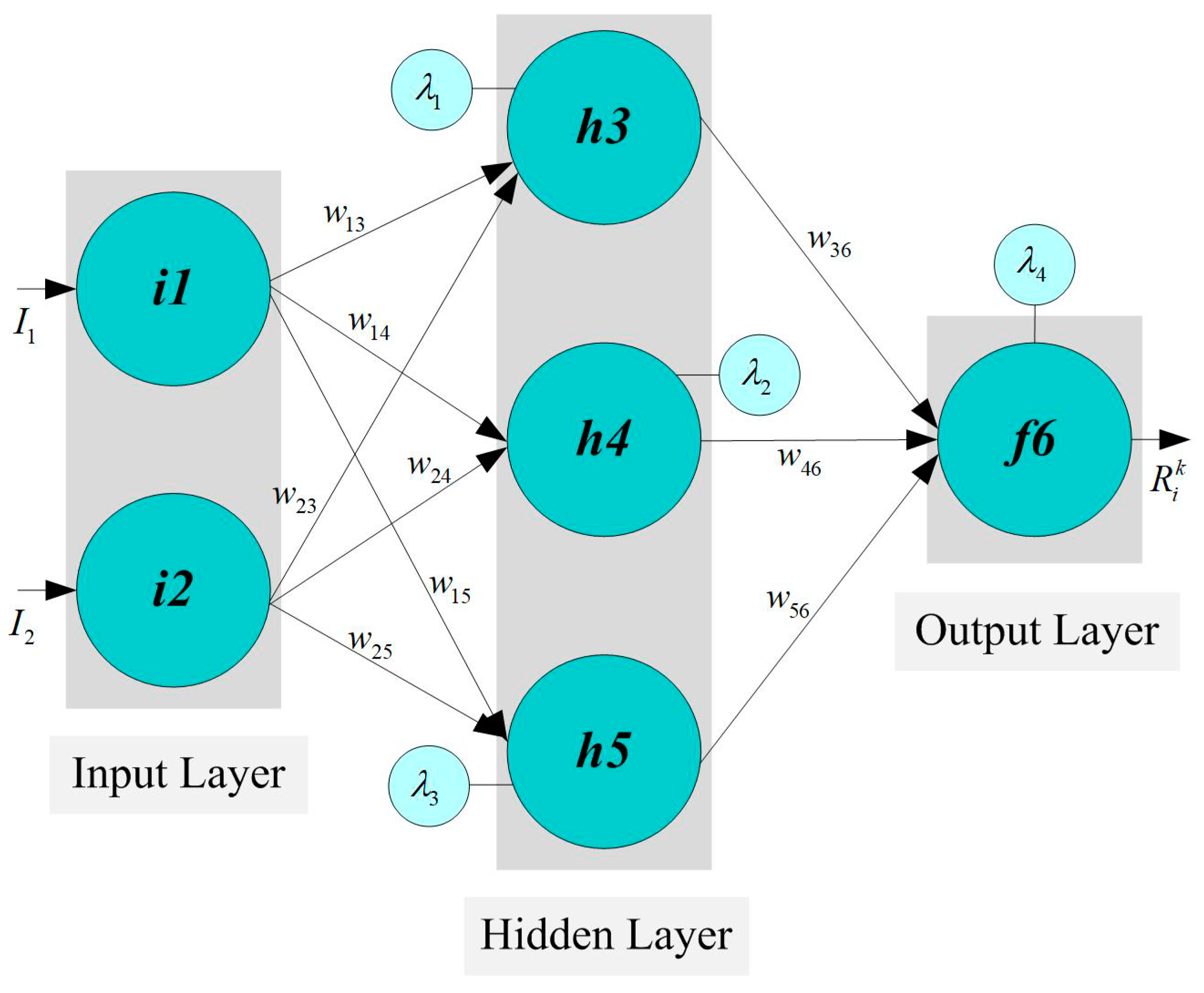
An artificial neural network is a machine learning type that uses the biological neural network as an inspiration for study [28,40]. The critical point of using ANN is estimating a mathematical function that relies on a huge amount of data with undescribed behavior. It consists of a fair number of interconnected neurons that capture the input parameters and direct them into a learning algorithm to compute the output values. A multilayer perceptron (MLP) is a feed-forward operation mechanism and is the most commonly used model among ANN models [33,40]. The primary function of an MLP model is to assign a group number of inputs to suitable output nodes. From its name, MLP has many layers that are fully interconnected in directed graphical representation. An activation function is required to operate all nodes, excluding the input node, this function being mostly a nonlinear function, and some cases have a linear activation function. It is essential to mention that the back-propagation technique, one of the supervised learning algorithms, can be used to train the network in multilayer perceptron ANN.

Generally, N layers indicate that there are N non-input layers of processing units and N layers of weights since the input layer is excluded as stated before. Figure 10 is an example of multiple-layer MLP. The relationships between these layers is described in the following equations:

$$ou{t}_n^{(2)}=f^{(2)}\left({\displaystyle \sum _{j=1}^{z}ou{t}_j^{(1)}{w}_{jn}^{(2)}}\right)$$

(1)

$$ou{t}_j^{(1)}=f^{(1)}\left({\displaystyle \sum _{i=1}^{t}ou{t}_i^{(O)}{w}_{ij}^{(1)}}\right)$$

(2)

$$ou{t}_i^{(O)}=i{n}_i$$

(3)

where f is the activation function, w is the weighting factor, z is the number of neurons in the hidden layer, and t is the total number of inputs in the first layer.

Figure 10. ANN architecture representation [28,40].

The nonlinear activation functions in MLP provide flexibility to the model in order to capture the variations in action potentials of biological neurons. The activation function should be normalized and able to be mathematically differentiated. There are two main activation functions widely used in the field of ANN. These functions are hyperbolic tangent and logistic function, and both are S-curve functions (sigmoid function). Hyperbolic tangent ranges −1 to 1, while logistic function ranges 0 to 1. Each node is connected to another node in the next layer with weighting factor, and these factors as summed using the following formula:

$$w_{in}={\displaystyle \sum _{j=1}^z{w}_{ij}^{(1)}{w}_{jn}^{(2)}}$$

(4)

Training neural network models in power-demand forecasting could be done offline or online. Neural network offline training depends on the input–output set, which is prepared to learn the neural network, and the use of neural network with data outside the training range may cause false results. The use of online training makes the network adapt itself to change in the dynamics of the system. The data collected for online training could contain bad data due to sensor errors. The network will respond to the bad data and produce an output that endangers the operation of the whole system, and this is the main factor that limits the use of neural network to online application in practice. In this paper, ANN is used as an offline application to predict the next 24 h loads and the next-week hourly loads.

2.2.3. Decision Tree (DT)

Decision tree is an effective algorithm in machine learning inspired by identifying a certain pattern to data in order to sort or predict events such that the goal is to optimally construct the decision tree with minimum generalization error [22,29]. In fact, decision tree is a pattern classification for trained subsets or objects in which the values of the properties of these objects are tested [22]. Decision tree structure starts from the first or initial node and ends up at the downstream nodes. The property of every node in the decision tree is evaluated using gain-below methodology. The procedures of decision tree can be summarized in the following steps:

A-

Initial node is selected and assigned to a discretional attribute value A.

B-

The border value of A is determined and the partition entropy aroused by value A is calculated; after that, the minimum one will be selected.

C-

For all attributes, gain below will be calculated and the attribute that has highest gain will be considered. The selected attribute will be the sort basis for the tree and the decision tree will be expanded at this particular node.

D-

The procedures above will be repeated until two main points are reached:

1-

Every node has only one node left and this node is called leaf node where there is no more expansion.

2-

The gain factor reaches the stopping criterion where there is no more sorting process.

Decision tree inducers can be classified into two types or conceptual phases [29]:

1-

Growing and pruning phase like C4.5 [34], CART [28], and M5 [29].

2-

Growing phase like ID3 [31].

M5 algorithm, which is used in this work, was constructed by Quinlan in 1992 for inducing trees of regression models [34]. It works initially by constricting a tree using induction. In order to reduce the intra-subset variation for the class values under each branch, a splitting methodology is utilized. Then, a back-pruning technique from the leaves is performed. Lastly, a smoothing step is applied to avoid the discontinuities among the subtrees. For more detail regarding DT implementation, the reader may refer to [22,28,29,31,34,37].

2.3. Model Performance Criteria

Several performance criteria have been proposed in the literature to evaluate the performance of predictive models. Mean magnitude relative error (MMRE), which is the average of residual error by the actual value, is a very popular performance criterion, but it was criticized, because it is biased and caters to models that underestimate [41]. For this purpose, the coefficient of determination R² and mean absolute residual MAR are used as evaluation criteria. Moreover, the time that each model takes for training is also considered. When R² gets closer to 1 and MAR gets closer to the zero, the accuracy of the model is very high. MAR depends on the unit of the predicted value. For instant, if the unit of the predicted value in megawatts (106 watts), it is reasonable to have some kilowatts as an error.

R² (the coefficient of determination) is a number (equal or below 1) that describes how well the data fit the regression model. It varies from 1 (when the regression line passes through all the data) to 0 (when there is no correlation—poor correlation). Mean absolute residual is measuring how far the predicted values are to the actual values. Clearly, the model is accurate when MAR is getting lower.

$$R^2=1-\frac{{\displaystyle \sum _{i=1}^n{\left(y_i(t)-{\widehat{y}}_i(t)\right)}^2}}{{\displaystyle \sum _{î=1}^n{\left(y_i(t)-{\overline{y}}_i(t)\right)}^2}}$$

(5)

$$MAR=\left(\frac{1}{n}\right){\displaystyle \sum _{i=1}^n\left|y_i(t)-{\widehat{y}}_i(t)\right|}$$

(6)

where $y_i$ is the actual value, ${\widehat{y}}_i$ the estimated value, ${\widehat{y}}_i$ the average value of $y_i$ and n the total number of observations.

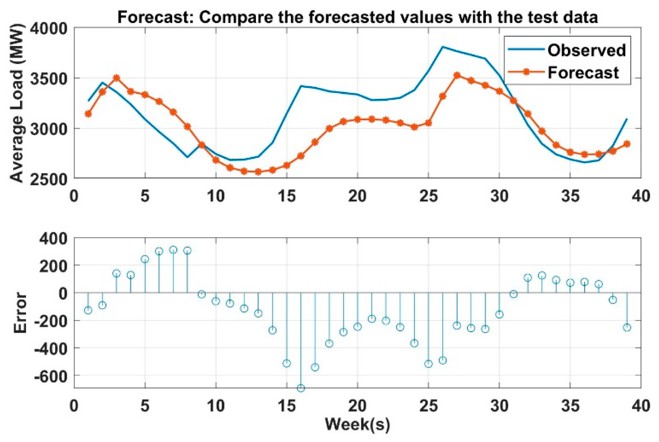
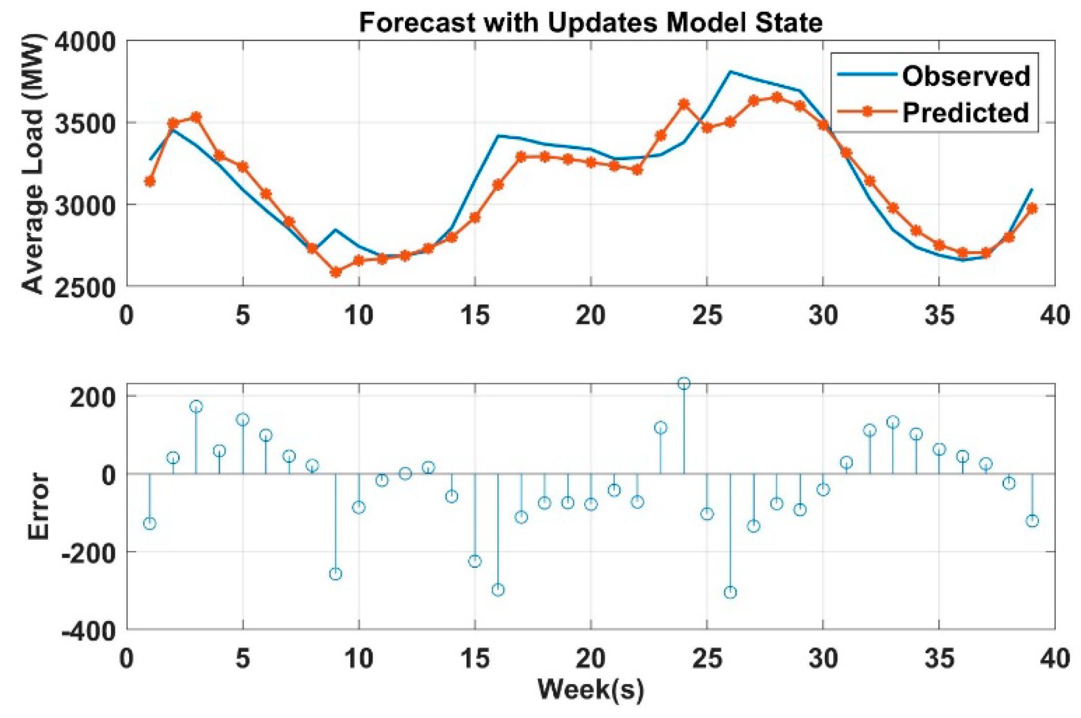
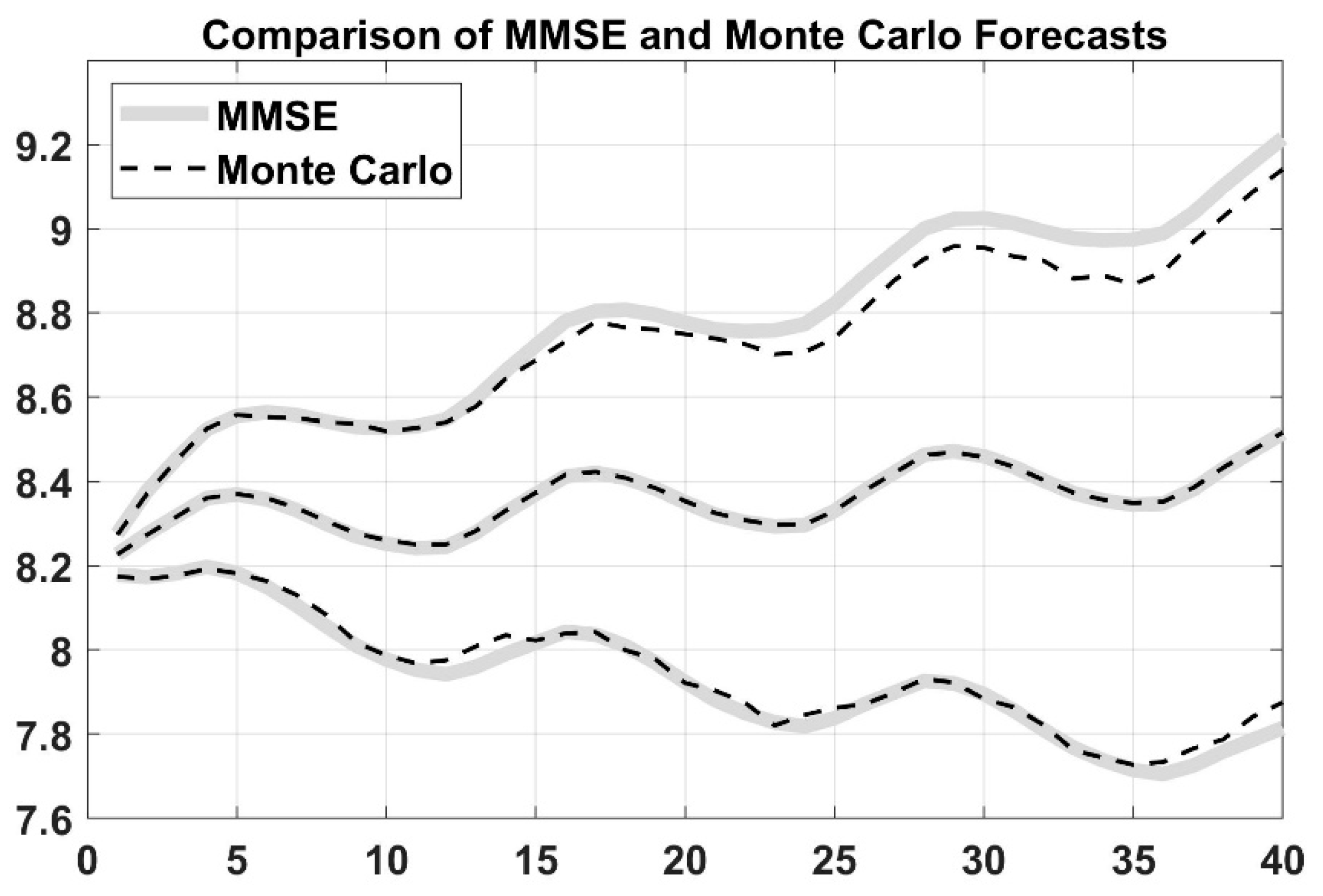
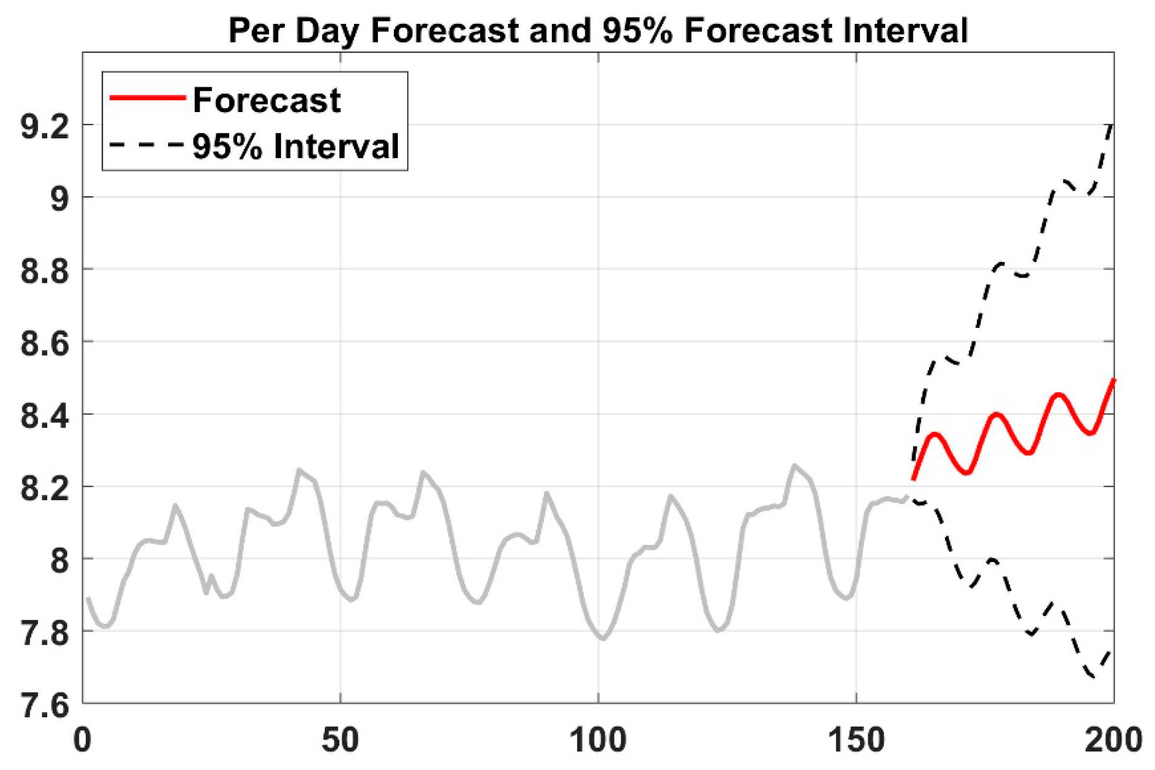
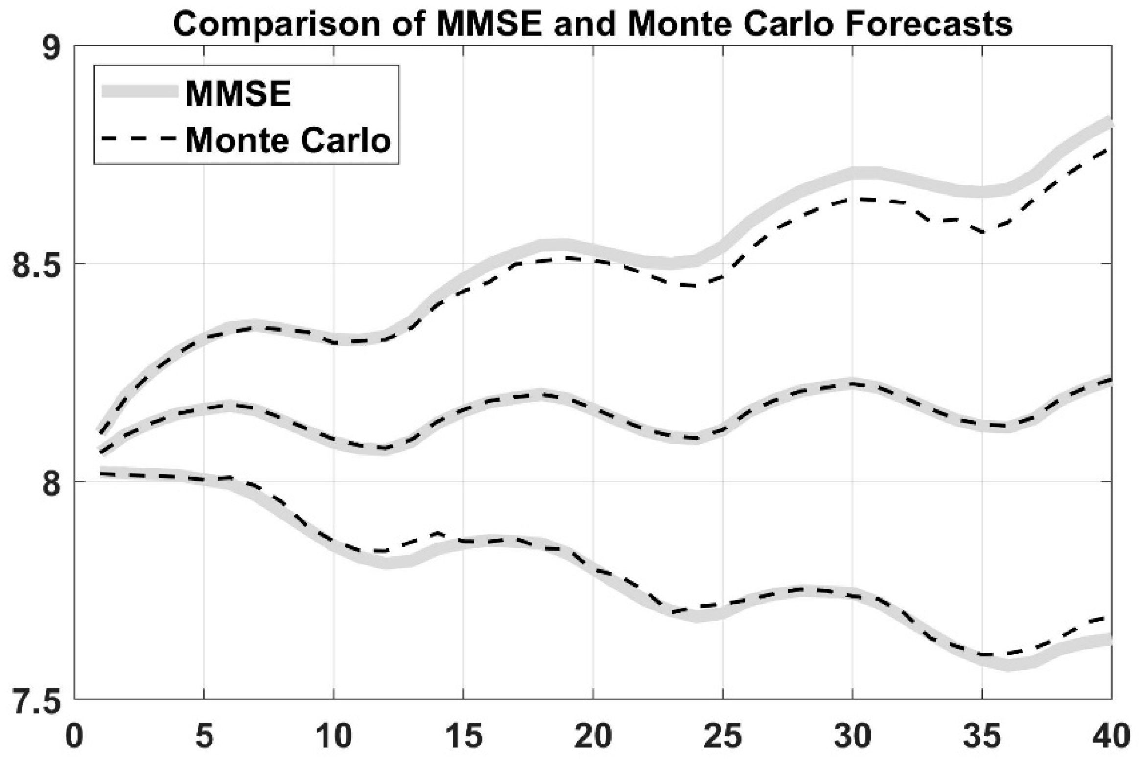
To examine whether these three models are statistically different or not, statistical tests (i.e., ARIMA and Monte Carlo method) are implemented. It is checked first if the conditions, such as the distribution of data and the value of variance for using parametric tests, are satisfied. If the results from the tests reveal that these conditions were not satisfied, then author used the nonparametric Kruskal–Wallis test to compare the different models.

3. Results and Discussion

The data are filtered from the outliers using Dixion’s Q test, and the clean datasets are utilized. Only nine data points are detected as outliers. Figure 8 (correlation diagram) shows how the relationship between some predictors and response is. It can be clearly seen from these figures that the relationship between the hourly load and last year load at the same time (LY) is linear. Furthermore, previous week load (PW), previous day load (PD), and average load for the 24 h prior to this time (P24H) are in linear relationship with the hourly load (response variable).

3.1. DNN-Based LF and Its Validation

3.1.1. DNN-Based LF

Based on the DNN model presented in Section 2.2.1, three distinct case studies have been analyzed in this section. These case studies are (1) per-hour forecasting, (2) per-day forecasting, and (3) per-week forecasting. Figure 11, Figure 12, Figure 13 and Figure 14, Figure 15, Figure 16, Figure 17 and Figure 18, Figure 19, Figure 20, Figure 21 and Figure 22 show the DNN performance analysis for case study 1, case study 2, and case study 3, respectively. The training progress representation for per-hour, per-day and per-week forecasting using LSTM based DNN is represented in Figure 11, Figure 15 and Figure 19 respectively, which shows all performance indices (e.g., validation limit, training type, start time, end time, epoch, iteration, maximum iteration, processing type, learning rate, etc.) of the DNN. In this study, following parameters are used for DNN model: numFeatures = 1; numResponses = 1; numHiddenUnits = 200; layers = […sequenceInputLayer (numFeatures), lstmLayer (numHiddenUnits), fullyConnectedLayer (numResponses), regressionLayer]; trainingOptions (‘adam’, …‘MaxEpochs’, 250, …‘GradientThreshold’, 1, …‘InitialLearnRate’, 0.005, …‘LearnRateSchedule’, ‘piecewise’, …‘LearnRateDropPeriod’, 125, …‘LearnRateDropFactor’, 0.2, …‘Verbose’, 0, …‘Plots’, ‘training-progress’).

Figure 11. Training progress representation for per-hour forecasting using LSTM-based DNN.

Figure 12. Per-hour forecast of future time series.

Figure 13. Comparison of per-hour forecast future time series with test data (observed value).

Figure 14. Comparison of per-hour forecast future time series using updated DNN model with test data (observed value).

Figure 15. Training progress representation for per-day forecasting using LSTM based DNN.

Figure 16. Per-day forecast of future time series.

Figure 17. Comparison of per-day forecast future time series with test data (observed value).

Figure 18. Comparison of per-day forecast future time series using updated DNN model with test data (observed value).

Figure 19. Training progress representation for per-week forecasting using LSTM-based DNN.

Figure 20. Per-week forecast of future time series.

Figure 21. Comparison of per-week forecast future time series with test data (observed value).

Figure 22. Comparison of per-week forecast future time series using updated DNN model with test data (observed value).

The proper completion of the training process for the forecast of future time series using the LSTM-based DNN model is represented in Figure 12, Figure 16 and Figure 20 for hourly, daily, and weekly, respectively. In these figures, blue lines represent the forecast (observed) values and red lines the forecast future value. The comparison of per-hour, per-day, and per-week forecast future time series with test data (observed value) is represented in Figure 13, Figure 17 and Figure 21, respectively, which show high correlation with each other, and the error value is very minimal for all data points: −200 to 200 only.

After this analysis, DNN model is updated with the observed new values and results are compared in between forecast with updated model state and observed value. Figure 14, Figure 18 and Figure 22 show the comparison of per-hour, per-day and per-week forecast future time series using updated DNN model with test data (observed value), which is more acceptable in performance limit.

As per the above explanation for the obtained results using DNN and its updated version, a comparative demonstration is tabulated in Table 3, which shows the result demonstration during testing phase conditions for all cases load forecasting. From the comparison, it is clear that the proposed DNN-based results are acceptable for further implementation on the actual site.

Table 3. DNN Based Result Demonstration with and without Updating the DNN Models.

Type of Forecasting	Testing Phase Result Demonstration
	DNN Model	Updated DNN Model
Per-hour forecasting	11.58186	4.08530
Per-day forecasting	16.93268	4.22537
Per-week forecasting	29.62043	15.00319

3.1.2. Validation Based on ARIMA and Monte Carlo Method

In this study, ARIMA and Monte Carlo (MC) approach [30,40] is used to validate the performance of DNN. Generally, ARIMA (p, D, q) model is used to forecast a non-stationary time-series dataset. Where, the parameters of ARIMA model are p, q and D are the order of autoregressive (AR), order of moving average (MA) and integrative part, respectively. For detailed information, reader may refer [30] and it can be represented as:

$${\mathsf{\Delta }}^D{y}_t=c+{\varphi }_1{\mathsf{\Delta }}^D{y}_{t-1}+\dots +{\varphi }_p{\mathsf{\Delta }}^D{y}_{t-p}+{\in }_t+{\theta }_1{\in }_{t-1}+{\theta }_q{\in }_{t-q}$$

(7)

MC is the model to create independent, random variables based on a probabilistic model. The development of the ARIMA and MC model is based on a similar dataset as used in the DNN model. The validated results are represented in Figure 23, Figure 24, Figure 25, Figure 26, Figure 27 and Figure 28. Figure 23, Figure 25 and Figure 27 represent the per-hour, per-day and per-week forecasting validation using the ARIMA model respectively. Moreover, Figure 24, Figure 26 and Figure 28 represent the per-hour, per-day and per-week forecasting validation using MC model respectively. The light gray color line represents the training dataset of the training phase whereas the red color line represents the forecast value during the testing phase of the ARIMA model (see Figure 23, Figure 25 and Figure 27). The forecast data is forecast in 95% forecast interval, which is highly acceptable. Similarly Figure 24, Figure 26 and Figure 28 represent the validation based on MC method (doted dark black color line) along with MMSE (light gray color line) based 2nd level of validation. All these figures show the high correlation between both methods and are acceptable for further use.

Figure 23. Per hour forecasting validation using ARIMA.

Figure 24. Per hour forecasting validation using MC.

Figure 25. Per day forecasting validation using ARIMA.

Figure 26. Per day forecasting validation using MC.

Figure 27. Per week forecasting validation using ARIMA.

Figure 28. Per week forecasting validation using MC.

3.2. ANN Based LF

Multilayer perceptron is used for ANN. There is one hidden layer. Theoretically, a single hidden layer as well as two layers with sufficient hidden neurons are capable to approximate any continuous function, and they are widely used and performing very well. Regarding the optimal selection of hidden neurons, there is no certain agreed formula and most of researchers depend basically on the experiments. However, there are several methods or rules of thumb for choosing the number of hidden neurons [42]. One of them that has been used in this work states that number of hidden neurons is the summation of number of inputs and outputs divided by two. Another rule of thumb states that depending on the problem, the number of hidden neurons is between one-third the number of input neurons to perhaps two or three times the number of input neurons. On the basis of these methodologies, we tested the problem twice, with one hidden layer and with two hidden layers. For single hidden layer, it has been found that the optimal number of neurons in single hidden layer is seven. When the number of hidden neurons increases above seven, the MAE increases. Figure 29 shows the variation of MAE with the number of hidden nodes. Learn rate and momentum are 0.3 and 0.2, respectively. Leave-one-out cross validation is utilized in neural network, as well. Mean absolute residual for the single hidden layer is 0.0558 kW and the coefficient of determination R² is improved to reach 0.958. Moreover, the performance with variation of hidden layers is represented in Figure 30.

Figure 29. MEA versus hidden layer neurons performance curve.

Figure 30. MEA versus hidden layers performance curve.

In case of double hidden layers, the experiments revealed that the optimal number of hidden neurons that gives minimum MAE is eight neurons in the first layer and six neurons in the second layer as shown in Figure 6. Mean absolute error is 0.051 kW and the coefficient of determination R² is 0.966.

3.3. DT Based LF

For the same data used in DNN, ANN, decision tree based predictive tool is utilized to predict hourly load. M5 technique is applied in this method as explained earlier. The optimal number of rules that minimize the mean absolute error was found to be 12 rules. So, the decision tree has 12 rules which means that we have 12 linear models that can forecast or represent the behavior of short-term power demand. Each rule is described in Table 4. The coefficients of each predictor in each rule are summarized in Table 5. Mean absolute residual was obtained from the decision tree model is 0.091 kW, which better than linear regression. The coefficient of determination R² is 0.904.

Table 4. Rule Characteristics.

Rule No.	Rule Characteristics
1	LY ≤ 2889, P24Hr ≤ 3039.3, Temp ≤ 18
2	LY ≤ 2889, P24Hr ≤ 3039.3, Temp > 18
3	LY ≤ 2889, P24Hr > 3039.3
4	LY > 2889, AP ≤ 100, PD ≤ 2758.2
5	LY > 2889, AP ≤ 100, PD > 2758.2
6	LY > 2889, AP > 100, P24Hr ≤ 3017.2
7	LY > 2889, AP > 100, P24Hr > 3017.2
8	LY ≤ 3584, AP ≤ 99.9
9	LY ≤ 3584, AP > 99.9
10	LY > 3584, AP ≤ 100
11	LY > 3584, AP > 100
12	LY > 3742

Table 5. The Coefficients of Each Predictor In Each Rule.

Attributes/Rule No.	LY	PW	PD	P24Hr	Temp	DT	Hum	WS	AP	OHEP	Constant
1	0.58	0.17	−0.26	0.19	16.53	−7.14	5.91	−0.91	11.24	−1.77	−1127.98
2	0.70	0.17	−0.26	0.19	23.81	−7.14	6.66	−0.91	11.24	−1.77	−1588.60
3	0.75	0.17	−0.26	0.19	17.57	−7.14	3.67	−0.91	11.24	−2.80	−1317.36
4	0.54	0.30	−0.23	−0.01	11.49	−7.14	—	−0.49	11.24	−1.98	−133.78
5	0.54	0.30	−0.22	0.20	11.49	−7.14	—	−0.91	11.24	−1.98	−797.84
6	0.76	0.34	−0.46	0.08	11.49	−7.14	—	−0.91	11.24	−1.98	−449.59
7	0.72	0.34	−0.43	0.08	11.49	−7.14	—	−0.91	11.24	−1.98	−426.06
8	1.14	0.12	−0.23	−0.18	16.73	−24.59	3.57	−0.87	−9.02	−1.97	964.80
9	0.93	0.08	−0.28	−0.18	28.95	−47.47	1.22	−0.87	24.24	−1.97	−1053.00
10	0.54	0.03	−0.21	−0.22	11.68	−18.37	0.72	−0.87	28.96	−9.37	289.99
11	0.54	0.03	−0.43	−0.22	11.68	−18.37	0.72	−0.87	28.96	−6.18	937.13
12	1.06	0.03	−0.34	−0.22	10.35	−16.88	0.72	−1.48	29.61	−0.39	−1526.00

3.4. Result Comparison and Validation

From Table 6, it is clear that the DNN model outperforms the other models based on the MAR and R² criteria. ANN model has the lowest MAR in single and double layers which are 0.0558 and 0.051, respectively. In addition, DNN models have the highest R² values.

Table 6. Comparison between DNN, ANN, and DT.

Model	R2	MAR	Model Building Time	Training Time
DNN	0.985	0.014	0.0002 s	32–33 s
ANN (1)	0.958	0.0558	0.42 s	1 min, 17 s
ANN (2)	0.966	0.051	0.42 s	3 min, 13 s
DR	0.904	0.091	0.16 s	15.2 s

However, DNN also took shortest time for generating and training the model compared to the other methods. Decision tree algorithm has lower MAR value than regression but higher than ANN, and the time to build and train the model is lower than ANN. From the above results, all the techniques provides very good results since R² for them are relatively high and MAR is small. All analyses were performed in both MINITAB and WEKA environments on a laptop with an Intel (R) Core i5 processor and 4 GB of RAM.

4. Conclusions

Load forecasting in power system is a very important daily duty in the operation section. Many activities in power system (or in power system planning) used the output from load prediction models as an input to their operation. For an example, LF (based on 1 week to 1 year) is required for maintenance scheduling. Similarly, LF (based on 1 min to 1 week) is required for unit commitment analysis (UCA), economic load dispatch flow analysis (ELD-FA), and automatic generation control and scheduling (AGCS). Therefore, it is very crucial to build an accurate and efficient predictive model to handle the uncertainty caused by load fluctuation. In this paper, three predictive models are created to predict the power load for short term period (i.e., 24 h to one week) to meet the demand and supply equilibrium, which is very helpful to the maintenance scheduling, UCA, ELD-FA, AGCS and PS dynamic analysis. These models prove its effectiveness and accuracy to predict the load. DNN, artificial neural network, and decision tree-based prediction are used in this paper. DNN performance is also validated based on ARIMA and MC method. As shown in the results, LSTM based DNN has the higher coefficient of determination R² among all models, and it has the lowest mean absolute residual. However, ANN takes more time for building and training the models compared to the others. Decision tree-based prediction algorithm has R² equals to 0.9 which is lower than ANN. The mean absolute residual of the decision tree model is lower than MLR and higher than ANN. The lowest R² value compared to the other is for multiple log-linear regression and it also has the higher MAR. However, with respect to the time taken to develop the model, DNN is very fast compared with ANN and DT. Broadly speaking, in the field of large power system, it is acceptable to have a few kilowatts errors in the forecast load since the total load is measured by megawatts or gigawatts, and it can been seen the differences between the MAR are relatively small. After conducting the Kruskal–Wallis nonparametric test, one can conclude that there is statistical significant difference between all the models at 5% level of significance. This work is also validated with stochastic time-series methods such as ARIMA and MC simulation which are very useful in short term prediction as well. This work can be applied to predict the micro-grid operation in power system by forecasting both renewable resources output and the existing demand output and making multiple relationships between the sources and demands. To sum up, machine learning algorithms and regression analysis provide an efficient and fairly accurate estimation for the power system demand.