Possibilities of Integrating Adsorption Chiller with Solar Collectors for Polish Climate Zone

Abstract

Solar-powered adsorption chillers are a particularly interesting alternative to energy-intensive conventional refrigeration systems. Integration of the adsorption chiller with solar collectors is a very promising concept since the increase in solar radiation coincides with the increased demand for cooling. Such a solution is very economical and environmentally friendly. It also fits in with current trends related to energy policy and sustainable development. The article presents the results of tests conducted for a two-bed adsorption chiller integrated with solar collectors. The tests were performed on selected days of the summer period (July and August) at the KEZO Research Centre PAS in Jablonna (Poland). Based on the results obtained, the performance parameters of the adsorption chiller were determined, and the problems associated with the integration of all components of the system were identified and discussed. The values of the determined Coefficient of Performance (COP) and cooling capacity for the tested adsorption chiller are, depending on the day on which the tests were conducted, from 0.531 to 0.692 and from 5.16 kW to 8.71 kW, respectively. Analysis of the test results made it possible to formulate conclusions related to the design of integrated systems of adsorption chillers with solar collectors.

1. Introduction

The demand for cooling, and thus the number of cooling systems being installed, is growing rapidly [1,2]. This is influenced, among other things, by global warming, which manifests itself through increasing average temperatures on the Earth and increasingly frequent temperature extremes. The global population growth, the increasing urbanisation and economic development additionally contribute to an intense increase in the demand for cooling. The thermal comfort of building occupants is a factor that significantly affects their productivity and well-being, and for this reason, too, air conditioning is becoming increasingly common [3]. Currently, it is electrically powered compression refrigeration systems that are most commonly used. Their advantages, which certainly include high efficiency and a relatively low price, are increasingly weakened by the disadvantages that alternative sources of cooling are devoid of. One of these is the high electricity consumption. A report by the International Institute of Refrigeration in Paris indicates that the refrigeration sector consumes about 20% of electricity globally [2]. The electricity required to power traditional chillers is primarily generated by burning fossil fuels [4]. This means that the production of cooling indirectly contributes to climate change. In 2019, air-conditioning units alone accounted for about 8.5 per cent of global electricity consumption generating 1 GT of CO₂ emissions into the atmosphere [5]. Additionally, during the summer period, traditional electrically powered chillers contribute to a more frequent occurrence of the peak load of the power system. Disadvantages of the traditional refrigeration systems also include the use of synthetic refrigerants. If leaked into the environment, they can contribute to the greenhouse effect and ozone depletion [6]. These disadvantages of conventional refrigeration systems have necessitated the search for alternative cooling methods. These include absorption and adsorption cooling systems. Adsorption refrigeration systems are typically supplied with low-temperature heat with a temperature between 50 °C and 90 °C [7,8], which can be waste heat obtained from solar energy or geothermal energy [9]. Consequently, adsorption chillers are a very promising alternative to conventional refrigeration technologies.

The fact that adsorption chillers are powered by low-quality heat is crucial to the broad prospect of integrating these devices into many types of systems. The utilisation of waste heat enables more efficient use of primary energy. For example, Sztekler et al., in their publication [10], described the possibility of integrating an adsorption refrigeration system with a gas turbine. Further, Krzywanski et al. [11] presented simulation and optimisation results for a two-bed adsorption chiller integrated into a single system with medium- and high-temperature buffer tanks, borehole thermal energy storage, thermal energy storage tank, a high-temperature heat pump and photovoltaic panels. In addition to the management of waste heat, the use of low-temperature heat to drive adsorption systems also enables the use of heat that is extracted from renewable resources in this form. One of such sources is solar energy.

The possibility of integrating adsorption chillers with solar thermal collectors has been described in numerous publications. There has been a growing interest in this subject for many years. Many simulations have been performed and prototypes made of this type of system in different parts of the world. The surge of interest in these issues is reflected in the graph shown in Figure 1. An increase in citations has been observed from zero in 2000 to more than 500 in 2021. The number of published papers has also increased. The highest number of publications was recorded for the year 2017. An increase in the number of published papers was again observed between 2019 and 2021 [12].

It is expected that the interest in the possibility of using heat from solar collectors to power adsorption chillers will increase significantly in the coming years. The integration of these two devices into a single system provides the unique benefit of being able to produce cooling using solar energy. The recorded increase in cooling demand over the course of the day coincides with the increase in solar irradiance. In locations where access to electricity is limited or impossible and solar irradiance is high, solar-powered adsorption chillers will enable the storage of food products, vaccines or medicines and provide cooling of rooms [13]. One of the characteristics of adsorption refrigeration systems is that their operation is not significantly affected by fluctuations in supply water temperature [14]. This is a major advantage in the context of integration with solar thermal collectors [15]. A system supported by an additional heat source or suitable heat storage is a versatile solution to stabilise the availability of solar energy. Solar power can be provided in two ways. The first one involves placing the adsorbent bed directly in the solar collector, while the second one is the use of a heat transfer fluid that circulates between the cooling system and the solar collector [15,16].

In a number of publications, researchers have proposed interesting design solutions. For example, Alelyani et al. [17] designed and analysed a single-tube adsorption chiller heated by solar energy. The structure was built with a solar vacuum collector and an adsorption chiller. It had a bed in the upper part and a condenser and evaporator in the lower part, as well as a heat extraction source. The authors performed an experimental investigation on the effect of the bed design on the performance parameters of the refrigeration system. A performance factor of 0.15 was obtained, and the bed design with a double tube filled with sorbent in a tube was found to be the most efficient. Moreover, it was found that in terms of the cost of the cooling produced, the system was not significantly different from a conventional system integrated with a photovoltaic system. Furthermore, Liu et al. [18] presented a solar tube chiller in the form of an integrated collector with an adsorbent bed. It was observed that the performance parameters changed depending on the length of the adsorption time. An optimum value for the adsorption duration of 45 min was selected. The COP and SCP values were then equal to 0.258 and 8.15 W/kg, respectively. The authors also compared the performance parameters of the device for the cases when silica gel and zeolite SAPO-34 were used as the adsorbent. They reported that the system achieved better performance for silica gel. Bouzeffour et al. [19] described an adsorption chiller system using a silica gel–water pair with a tubular bed directly integrated with a solar collector. The authors obtained a COP in the range of 0.083 to 0.09 during the testing. Further, Lattieff et al. [20] used two-tube and vacuum solar collectors with a total surface area of 4 m² integrated with a single-bed adsorption chiller. The tests were carried out in the Middle East. The authors performed tests on the system to determine the most favourable hot water flow rate. This was found to be 30 L/min. For an adsorption time of 10 min, a COP of 0.56 and an SCP of 39 W/kg were obtained. The temperature values of the heat source and the chilled water at the evaporator outlet were equal to approx. 75 °C and approx. 6.6 °C, respectively. Qadir et al. [21] published a paper on the issue of modelling the operation of a solar-powered two-bed chiller with adaptive cycle time. The length of the cycle time has a very significant impact on the performance parameters and is dependent on the operating conditions of the device. The use of such a solution enables real-time selection of the most favourable cycle time depending on the solar irradiance. The authors compared the performance parameters for a chiller operating without adaptive cycle time and in the case where adaptation of the cycle time occurs. The use of variable adsorption/desorption cycle time resulted in a 19% increase in average SCP and a 66% increase in average COP. The maximum COP could then reach a value of 1.06. Furthermore, Pan and Wang [22] performed a simulation of a two-bed adsorption chiller integrated with solar collectors, on the basis of which they optimised the duration of the cycle. The authors compared two scenarios where in the first case, the cycle time was constant with increasing hot water temperature, and in the second case, it was variable. They found that the COP increased as a result of using the variable duration of the cycle while the SCP remained almost unchanged. Rouf et al. [23] investigated a three-bed adsorption chiller integrated with solar collectors. The results were compared with those obtained for a two-bed adsorption chiller operating under the same conditions. It was found that the three-bed chiller could operate with fewer solar collectors and longer after sunset compared with the two-bed chiller. More favourable performance parameters were also obtained for the three-bed chiller. Alahmer et al. [24] carried out simulations for a two-bed adsorption chiller integrated with vacuum tube collectors under the climatic conditions prevailing in Perth (Australia) and Amman (Jordan). The most favourable collector parameters were determined, including a collector surface area of 36 m² and an inclination angle of 30°. The average COP and cooling capacity for both locations were determined. These were 0.491 and 10.3 kW for Perth and 0.467 and 8.43 kW for Amman, respectively. Jaiswal et al. [25] conducted a simulation study for a two-bed adsorption chiller with silica gel–water as the working pair, powered by heat from vacuum-tube collectors. It was found that the cooling capacity increases, and the average coefficient of performance decreases, with the increasing surface area of solar collectors. Parameters such as cycle time and the selection of an appropriate surface area of the collector were found to be crucial to the operation of the cooling system. Halon et al. [26] performed an experimental study of an adsorption chiller system powered by district heat and supported by heat from solar collectors. The use of two heat sources increased the cooling effect by three times compared with heat supplied from solar collectors only and by 14% compared with heat supplied from district heating only. Alahmer et al. [27] used a mathematical model of a two-bed adsorption chiller integrated with 38 m² parabolic concentrators to simulate the operation of a system installed in Western Australia. They obtained a COP of the system ranging from 0.4 to 0.55. It was shown that this type of investment could pay for itself within 11 years. El-Sharkawy et al. [28] made a mathematical model of a two-bed adsorption chiller powered by heat extracted from parabolic concentrators and operating in the Middle East. Simulations were performed for a system with and without a heating water buffer tank. Higher values of average cooling power and average COP were obtained for the first variant. Reda et al. [29] carried out an experimental study for a small system of a two-bed solar adsorption chiller with a silica gel–water working pair, with a cooling capacity of 8 kW. The system was equipped with parabolic solar collectors with a surface area of 36 m². It was found that an increase in the heating water temperature increases the cooling capacity and decreases the COP. An increase in chilled water temperature contributes to an increase in both the cooling power and the COP. A lowering of the temperature of chilled water caused an increase in the COP of the chiller by 40% and of the cooling power by 17%. Depending on the operating conditions of the chiller, COPs ranging from 0.43 to 0.63 and cooling power from 3.5 kW to 6.6 kW were obtained. Rouf et al. [30] published the results of a study conducted for a three-bed and a four-bed adsorption chiller powered by heat captured from parabolic concentrators. The use of adsorption chillers in such configurations enabled higher efficiencies to be achieved with lower quality heat extracted from the collectors. Chen et al. [31] discussed a configuration consisting of a single-bed adsorption chiller operating together with a parabolic solar collector equipped with a solar tracking system. The chiller used SAPO-34 zeolite and water as the working pair. The authors embarked on finding the best duration of adsorption considering the maximisation of the SCP and COP of the system. Elsheniti et al. [32] tested the feasibility of using aluminium fumarate in a system consisting of a two-bed adsorption chiller, a hot water buffer tank and 27 vacuum-tube collectors with an effective surface area of approx. 1.95 m². Among other things, the COP, SCP and SDWP values were compared depending on the fin spacing of the heat exchanger, the adsorbent used (aluminium fumarate or silica gel) and the month in which the system was operated. The effect of the temperature of chilled water at the evaporator inlet and of the cycle time on the performance parameters was also checked. In their paper, Robbins and Garimella [33] presented a stand-alone system of a single-bed chiller using activated carbon–ammonia as the working pair integrated with a solar collector with a surface area of 1 m². COPs ranging from 0.12 to 0.24 and cooling capacities ranging from 25 W/kg to 80 W/kg were obtained. Asif Sha and Baiju [34] performed a simulation of the operation of a two-bed adsorption chiller using activated carbon–ethanol as the working pair integrated with parabolic concentrators. The authors obtained a maximum COP of 0.68. A comprehensive and detailed review of the literature on solar-powered adsorption chillers is presented in [35]. The authors described numerous systems with a division into the working pairs used in them. They also included an analysis of hybrid systems and sorption heat stores.

The review of the literature on the integration of adsorption chillers with solar thermal collectors confirms that there is much effort put into developing the technology of solar adsorption chillers and that much has still to be performed in this area. As a source of renewable energy available almost everywhere, solar energy is generating reasonable interest among researchers concerning its use together with adsorption refrigeration systems.

This paper analyses the possibilities of using solar collectors to power an adsorption chiller under the climatic conditions prevailing in Poland. The investigation was conducted during the summer season (July and August), i.e., a cooling season in Central and Eastern Europe. The study presents the performance characteristics of such a system located in Poland obtained based on measurements and tests carried out for a number of selected days. Time periods were analysed, when the installation works properly and days when the cooperation of the chiller and collectors is ineffective, illustrating the problems associated with the operation of such systems. The main objective of the investigation was to determine the cooling coefficient of performance (COP) and the cooling power of the device operating in the climate zone analysed. In addition, the results of the research made it possible to determine the validity of using systems of this type under the climatic conditions of Poland. The results represent a further step in planning the transformation of the energy sector in Poland, with particular emphasis on the refrigeration industry, the growing role of renewable energy sources and the need to implement a circular economy.

2. Materials and Methods

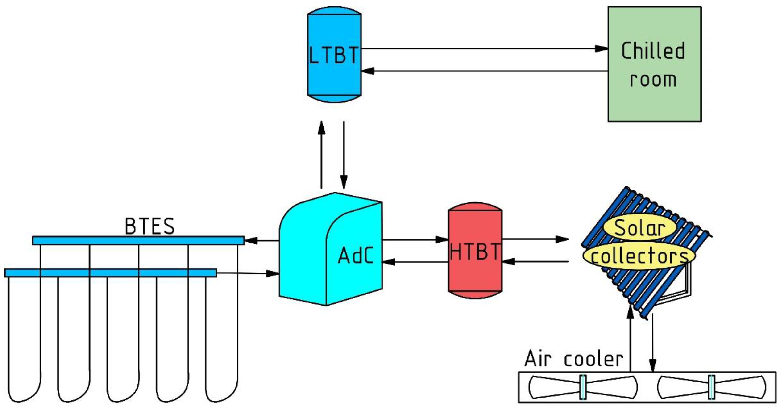
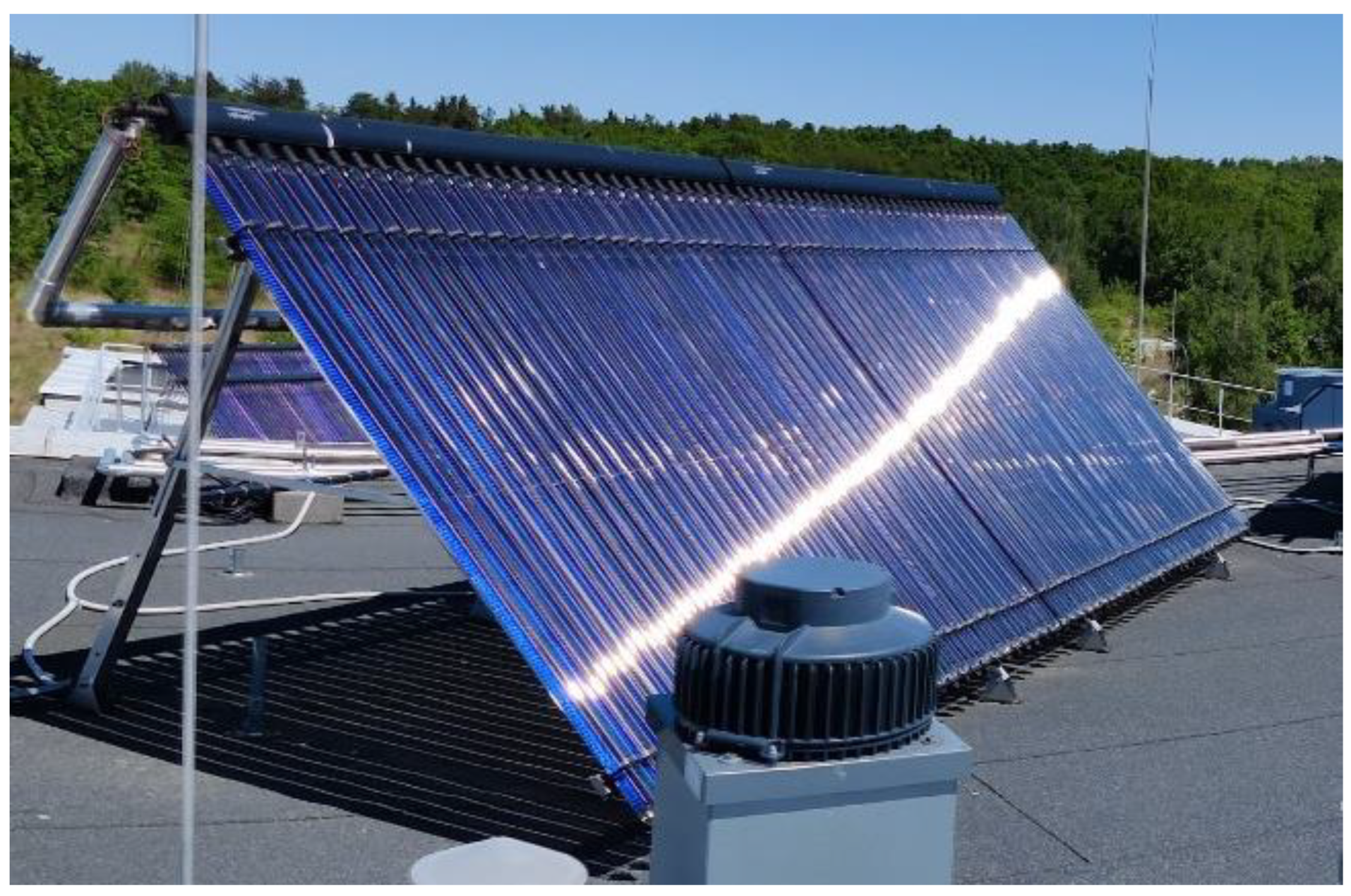
2.1. Description of the System

The system, being the subject of this investigation, is located at the PAS Research Centre Energy Conversion and Renewable Resources in Jablonna (central Poland, 52.378062° N, 20.928937° E). The system consists of four basic components, i.e., an adsorption chiller (SorTech, eCoo 2.0, Fahrenheit AG, Halle, Germany), solar thermal collector units (Kingspan Thermomax DF400 and HP 400, Kingspan Environmental, United Kingdom), and a borehole thermal energy storage (BTES) system and buffer tanks. The system is equipped with 2 buffer tanks, a high-temperature tank and a low-temperature tank. Each of the tanks has a capacity of 5 m³. The buffer tanks work directly with the adsorption chiller. The high-temperature buffer tank (HTBT) is responsible for managing the excess heat supplied by the solar thermal collector unit and maintaining a constant heating water supply temperature during periods of reduced performance of the solar system. The second buffer tank is responsible for managing the excess cooling energy when a lack of demand is signalled by the energy management system of the building being cooled. Excess heat generated as a result of adsorption is routed to the ground (BTES) by means of the medium-temperature (MT) circuit through a set of borehole heat exchangers, each of which is 80 metres deep. Protection against overheating of the solar collector unit is provided by an emergency cooling system equipped with an air-glycol exchanger (air cooler). A schematic of the system is shown in Figure 2.

The adsorption chiller that constitutes the central component of the system being described is based on a two-bed design. The chiller has two sections, a process section and an auxiliary section. The process section comprises two adsorption modules. The auxiliary section contains circulating pumps, piping and 3-way diverter valves serving 3 circuits, i.e., the heating water circuit (HT), the cooling water circuit (MT) and the chilled water circuit (LT). The working pair used in the chiller is water–silica gel. The basic parameters of the adsorption chiller tested are summarised in

Table 1. Technical data of SorTech eCoo 2.0 adsorption chiller [36].

Parameter	Unit	Value
Cooling capacity	kW	max. 16.0
COP	-	max. 0.65
Heating water temperature range	°C	50–95
Nominal heating water flow rate	L/h	2500
Cooling water temperature range	°C	max. 40
Nominal cooling water flow rate	L/h	5100
Chilled water temperature range	°C	min. 8
Nominal chilled water flow rate	L/h	2900

.

The heat source was provided by a Kingspan Thermomax vacuum tube collector unit located on the roof of the building. Figure 3 shows the solar collector unit in operation. The solar collector unit consists of 24 modules (13× DF400 30-way, 9× HP400 20-way, 2× HP 400 30-way) which are connected in parallel. The basic technical parameters of the solar collectors are summarised in

Table 2. Technical data of Kingspan Thermomax solar collector [37].

Parameter	Unit	DF400-30	HP400-20	HP400-30
Type	-	Direct flow	Heat pipe	Heat pipe
Max operating pressure	bar	8	10	10
Volume	l	5.6	1.2	1.7
Gross area	m2	3.23	2.13	3.20
Heat transfer fluid	-	water/glycol	water/glycol	water/glycol
Stagnation temperature	°C	313	166	166

.

The climatic data, i.e., ambient temperature (outdoor temp.) and intensity of solar radiation, were determined based on measurements taken at the meteorological station Warsaw Okęcie (52.167187° N, 20.967937° E). Figure 4 shows the average values of solar radiation intensity and outdoor temperature.

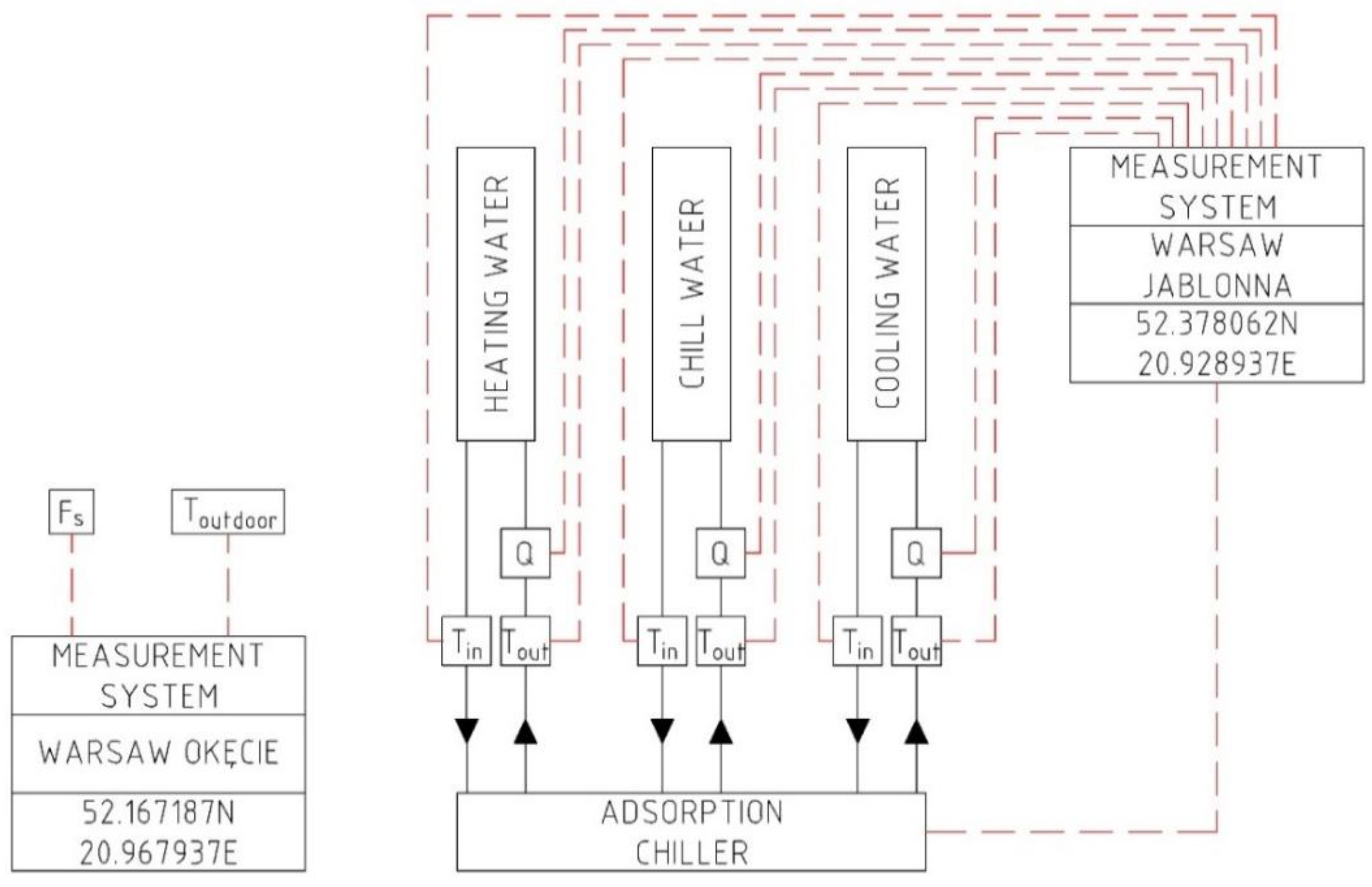
2.2. Methods

When using the measurement setup created, measurements were taken between 9 a.m. and 3 p.m. (9.00–15.00 h) during the summer months of July and August. During the analysis of the results, some problems related to the integration of the adsorption chiller with the solar collectors were noticed. Integration problems can be wildly shown during system operating hours from 9:00 a.m. to 3:00 p.m. The sampling time was 1 s. The characteristics of the measuring instruments are summarised in

Table 3. Technical data of the measuring instruments.

Parameter	Unit	Accuracy	Type
Temperature of cooling and heating water	°C	±0.2	Pt1000
Temperature of chilled water	°C	±0.2	Pt100
Flow rate	kg/s	0.5%	electromagnetic

. Figure 5 shows a schematic of the measurement systems used in this study. Both systems were located in close proximity to Warsaw. The first system was responsible for measuring outdoor temperature and solar radiation intensity. The second was used to measure the temperature and flow rate of the heating, cooling and chilled water circuits.

Based on the values obtained for the supply and return temperatures for each circuit and the mass flow rate, the values of the cooling capacity (Q_c) and heat demand (Q_h) were determined as described by the equations:

$${\mathrm{Q}}_{\mathrm{c}}={\mathrm{c}}_{\mathrm{p}}·{\stackrel{.}{\mathrm{m}}}_{\mathrm{chilled} \mathrm{water}}·\left({\mathrm{T}}_{{\mathrm{chilled}}_{\mathrm{in}}}-{\mathrm{T}}_{{\mathrm{chilled}}_{\mathrm{out}}}\right),$$

(1)

$${\mathrm{Q}}_{\mathrm{h}}={\mathrm{c}}_{\mathrm{p}}·{\stackrel{.}{\mathrm{m}}}_{\mathrm{heating} \mathrm{water}}·\left({\mathrm{T}}_{{\mathrm{heating}}_{\mathrm{in}}}-{\mathrm{T}}_{{\mathrm{heating}}_{\mathrm{out}}}\right),$$

(2)

where, c_p is specific heat of water of 4190 kJ/kgK, m_{chilled water} is mass flow rate of chilled water, T_{chilled in} is chilled water inlet temperature (return from LTBT), T_{chilled out} is chilled water outlet temperature from the chiller (supply to LTBT), m_{heating water} is mass flow rate of heating water, T_{heating in} is heating water inlet temperature (return from HTBT) and T_{heating out} is temperature at the chiller outlet (supply to HTBT). By using the values obtained, the temperature coefficient of performance (COP) was determined according to the equation:

$$\mathrm{COP}=\frac{{\mathrm{Q}}_{\mathrm{c}}}{{\mathrm{Q}}_{\mathrm{h}}},$$

(3)

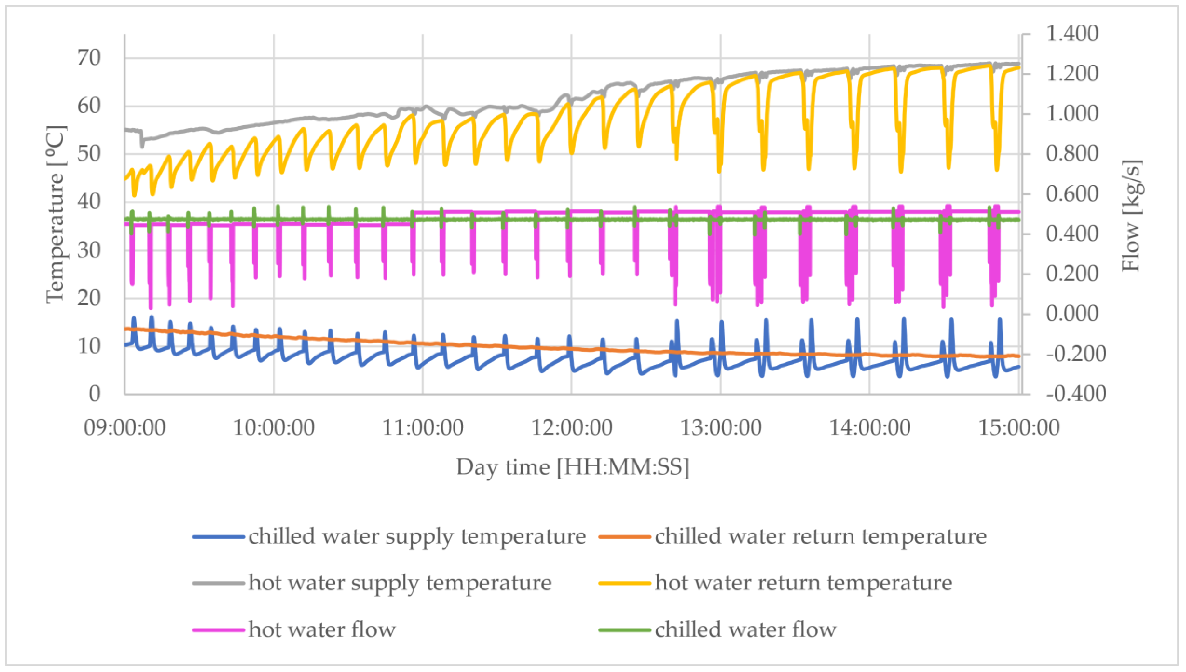
3. Results

The values measured in the course of the experiment made it possible to determine the cooling power and the heating power for each measuring point according to relations 1 and 2. For computational purposes, a constant value of specific heat of water of 4190 J/(kg/K) was assumed. Then, using Formula (3), the cooling coefficient of performance (COP) was calculated. The data obtained were analysed, and the extremes were discarded, i.e., values below 0 and above 1 for the COP, as well as negative values for the flows that were recorded at the point of bed switching in the chiller. The next step was to draw appropriate graphs for the selected time intervals showing the relations between the most important quantities occurring in the process. The graphs are presented and described in the following sections.

Figure 6, Figure 7 and Figure 8 show the results of the tests for 22nd July, which is the point of reference for the rest of the tests. On that day, the chiller operated with a 24 h removal of cooling, and therefore this is an example of correct integration with solar collectors when adequate removal of cooling and stable high solar irradiance are observed. When analysing the data in Figure 6, it should be noted that the chilled water flow rate is approximately constant at 0.471 kg/s, and any fluctuations are of the order of 10⁻³ kg/s. The periodic, sudden and short increases and decreases in the flow rate are related to the switching of the chiller cycles. The hot water flow rate, in turn, remains at 0.400 kg/s and is subject to cyclical fluctuations of approx. 0.20 kg/s, which, as in the case of chilled water, is related to the cycling of the adsorption chiller operation. On 22nd July, the chiller started producing chilled water at a temperature of approx. 18 °C, and towards the end of the day, this temperature was approx. 10 °C. This has to do with the fact that on 21st July, the building was also cooled around the clock, which resulted in the extraction of cooling from the chilled water storage tank. The chilled water temperature achieved at the end of the day indicates that the cooling capacity of the chiller exceeds the cooling load of the building, which allows storage of cooling for periods when there is no supply of solar radiation. Furthermore, an increase in the heating water temperature over time is also observed, which allowed the hot water flow rate to be maintained at the set value even despite a decrease in the value of the chilled water supply temperature. It should also be noted that on 22nd July the chiller was started up a short while before 9 a.m. so that until about 10:20 a.m. a start-up of the unit is observed resulting in a higher temperature gradient in the heating water circuit and shorter operating cycles.

Figure 7 shows the time course of the calculated values of thermal and cooling power and the meteorological data in the form of solar irradiance during the operating hours of the system. The cooling power for a chilled water flow temperature of approx. 18 °C reaches a maximum of approx. 12 kW, with a decrease in the generated cooling power over time down to a value of approx. 10 kW. This is related to the drop in the chilled water temperature to about 10 °C (Figure 9). It is also important to note the course of the change in the value of the heating power demand of the chiller, which reaches a maximum of approx. 30 kW between 9 and 10:30 a.m., while after 10:30 a.m., the maximum value is approx. 20 kW. This change is due to the shape of the hot water temperature curve (Figure 9). During the morning hours, the hot water has a supply temperature of approx. 55 °C and is subject to cooling down to even 35 °C during the process of desorption. In addition, it should be noted that on 22nd July, the chiller was started up a short while before 9 a.m., so the first hour of operation included still not fully stable operation.

The data in Figure 8 show the time course of change in the COP value. It should be noted that during the morning hours, the average COP value is lower than after 10:30 a.m. This is due to the higher value of heating power demand during these hours as compared with the rest of the chiller operating time. In addition, a decrease in the COP value over time is observed from 11 a.m. onwards, which is related to the drop in chilled water temperature as observed in Figure 9. Nevertheless, the average COP value varies between 0.4 and 0.7, which illustrates operation at nominal conditions and supports the assertion that the integration of the chiller with the solar collectors and the cooling plant is correct in the building on the day is considered.

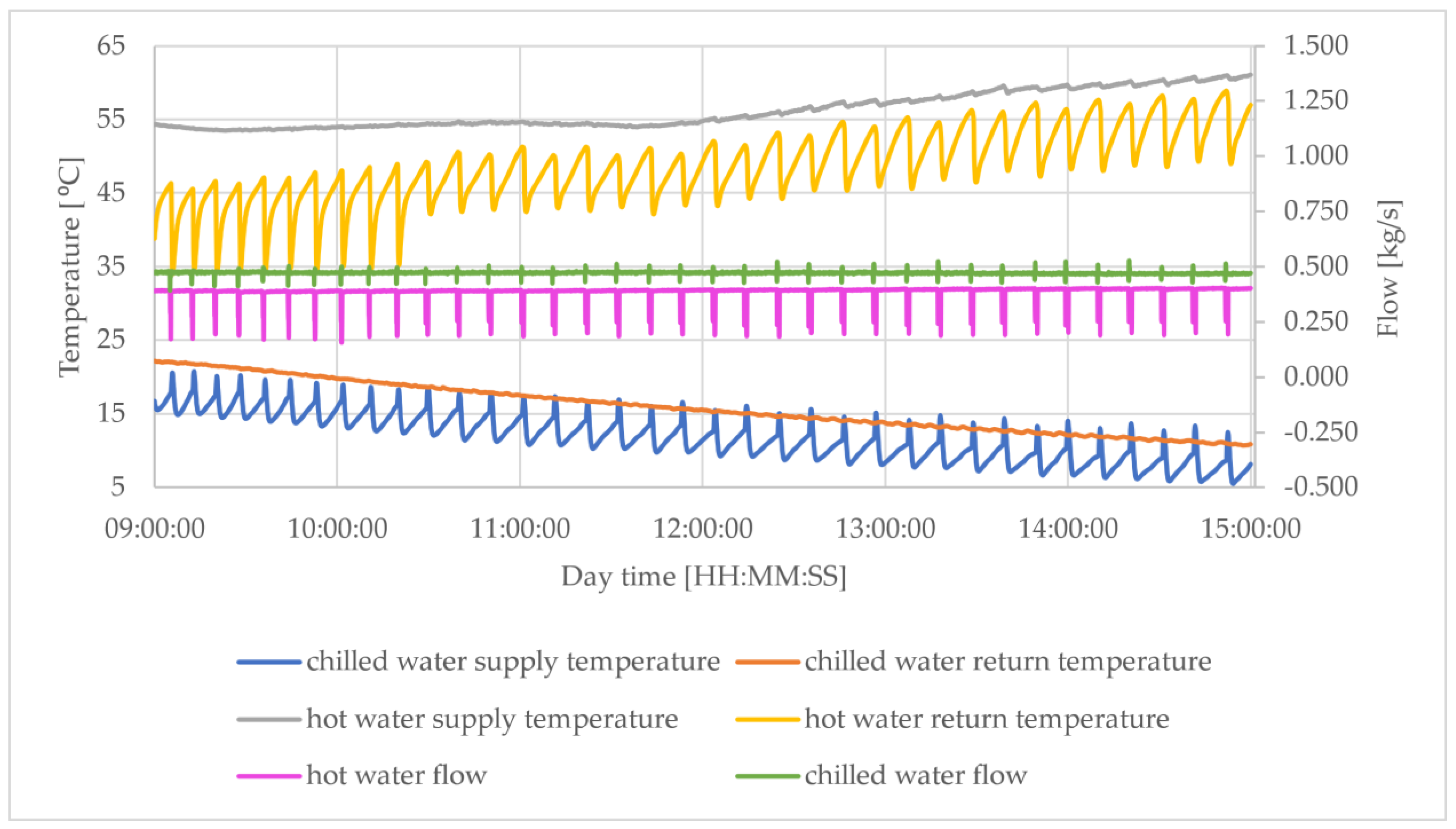
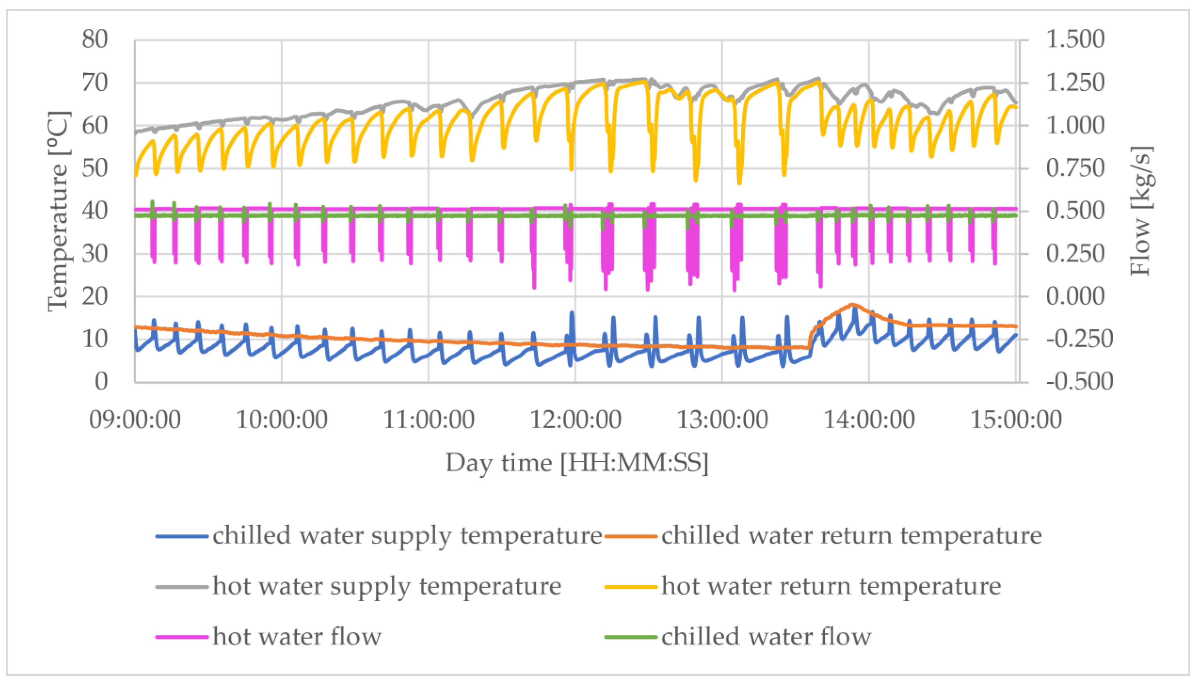
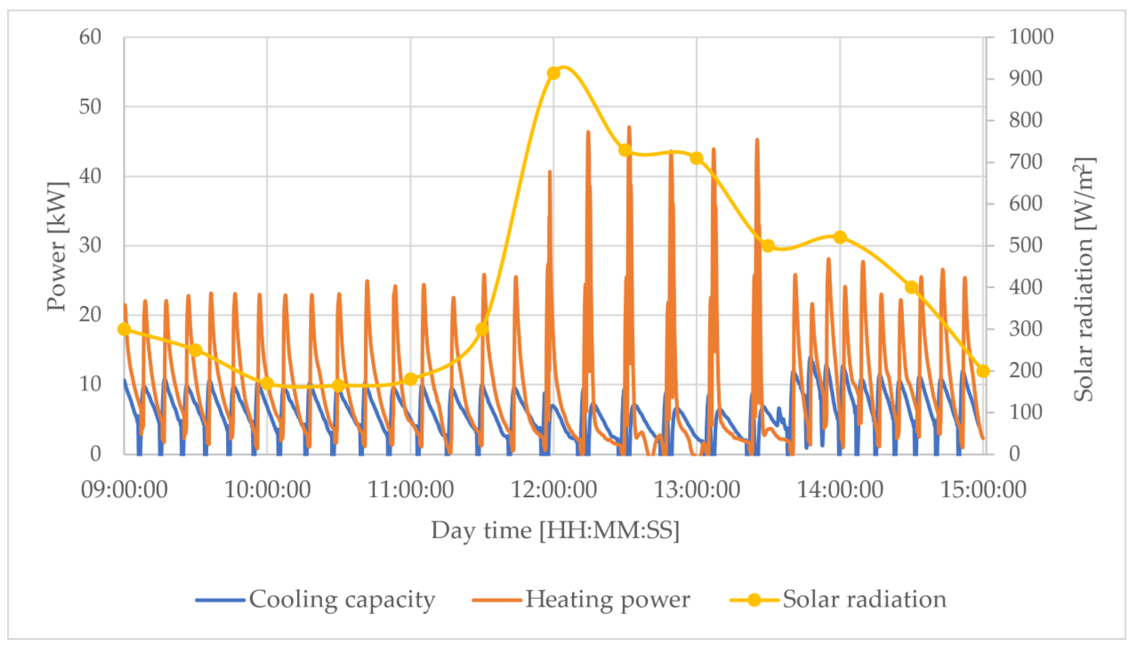
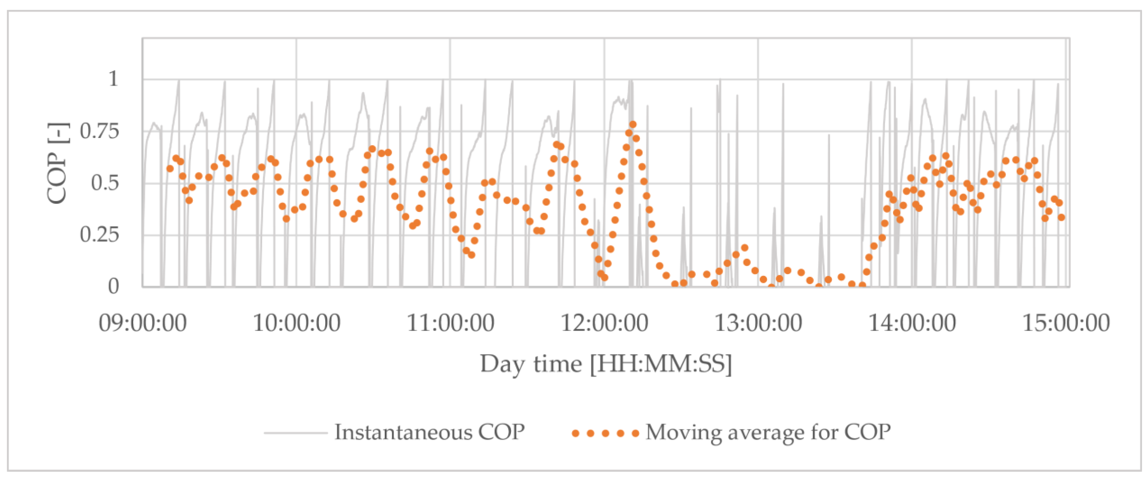
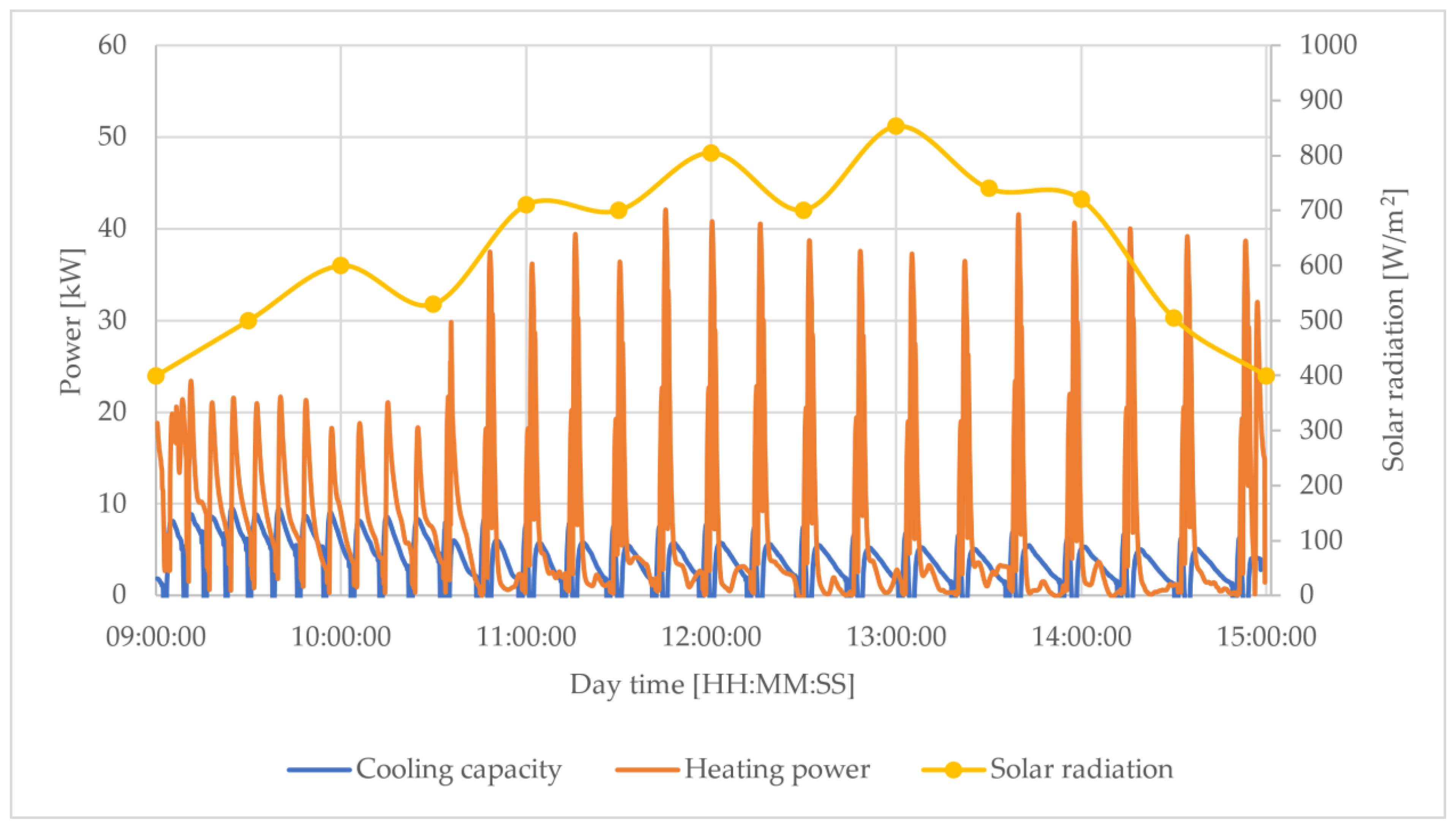
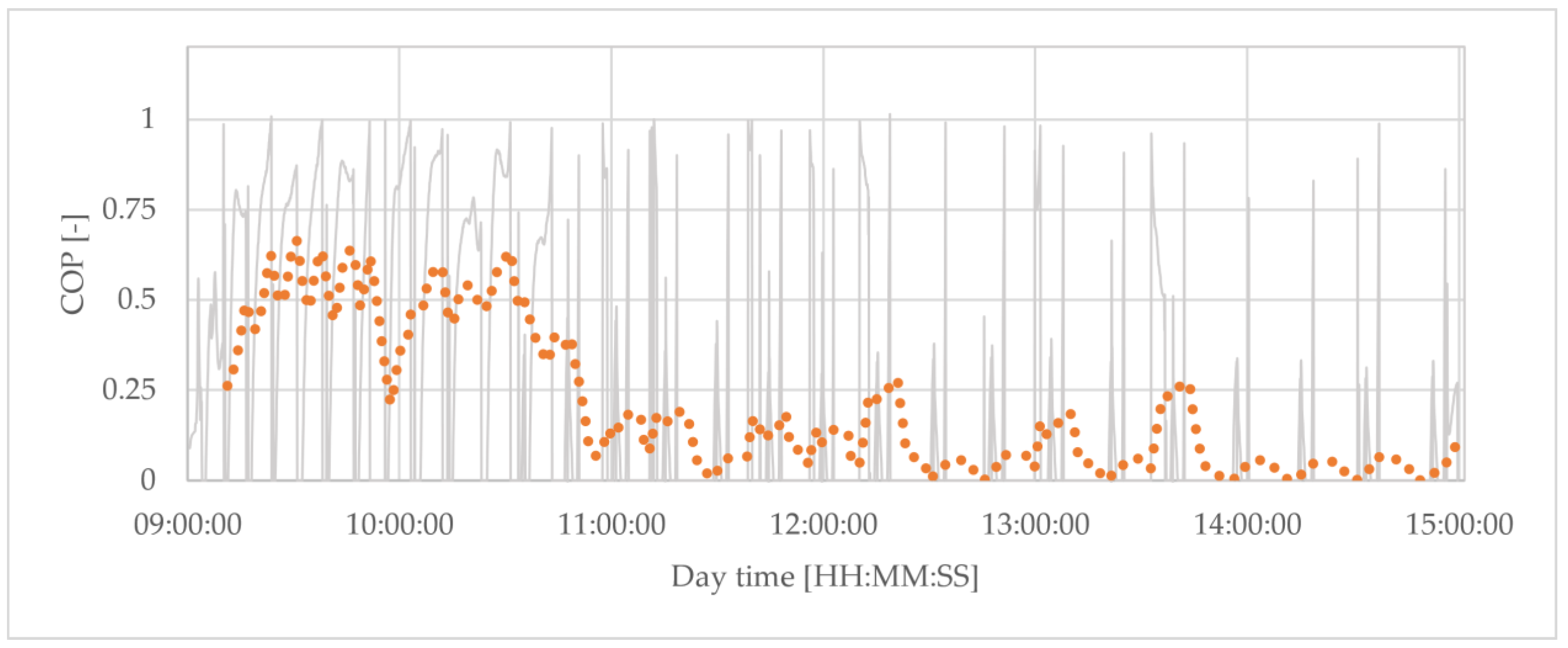
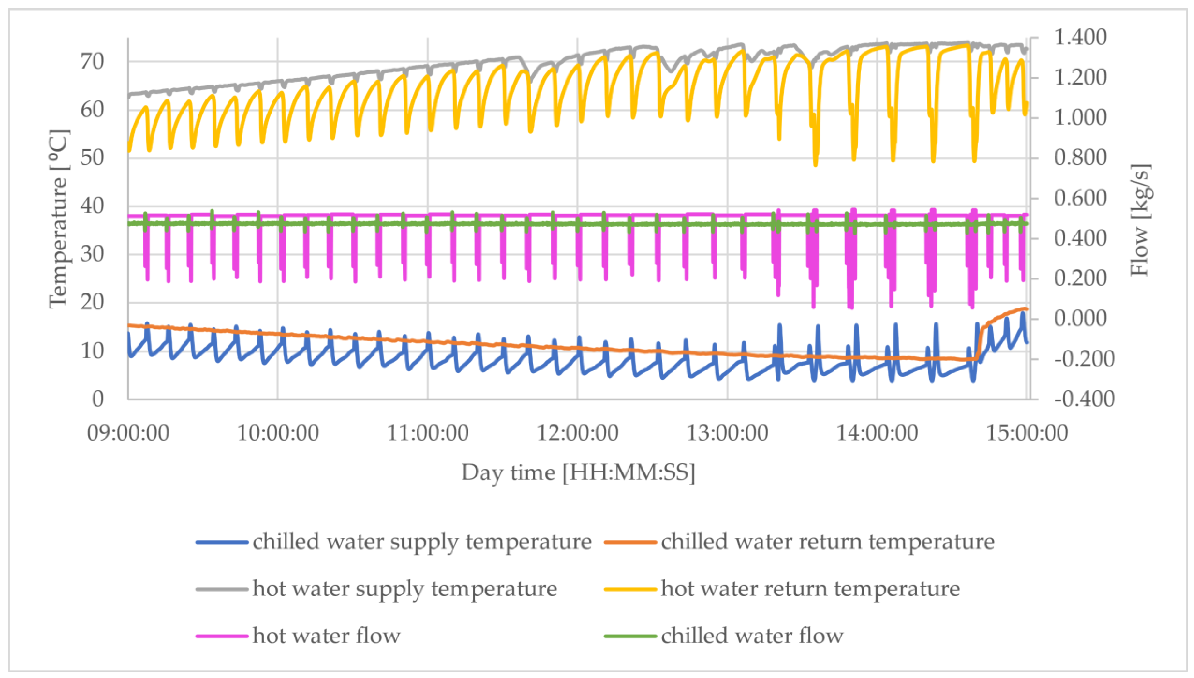
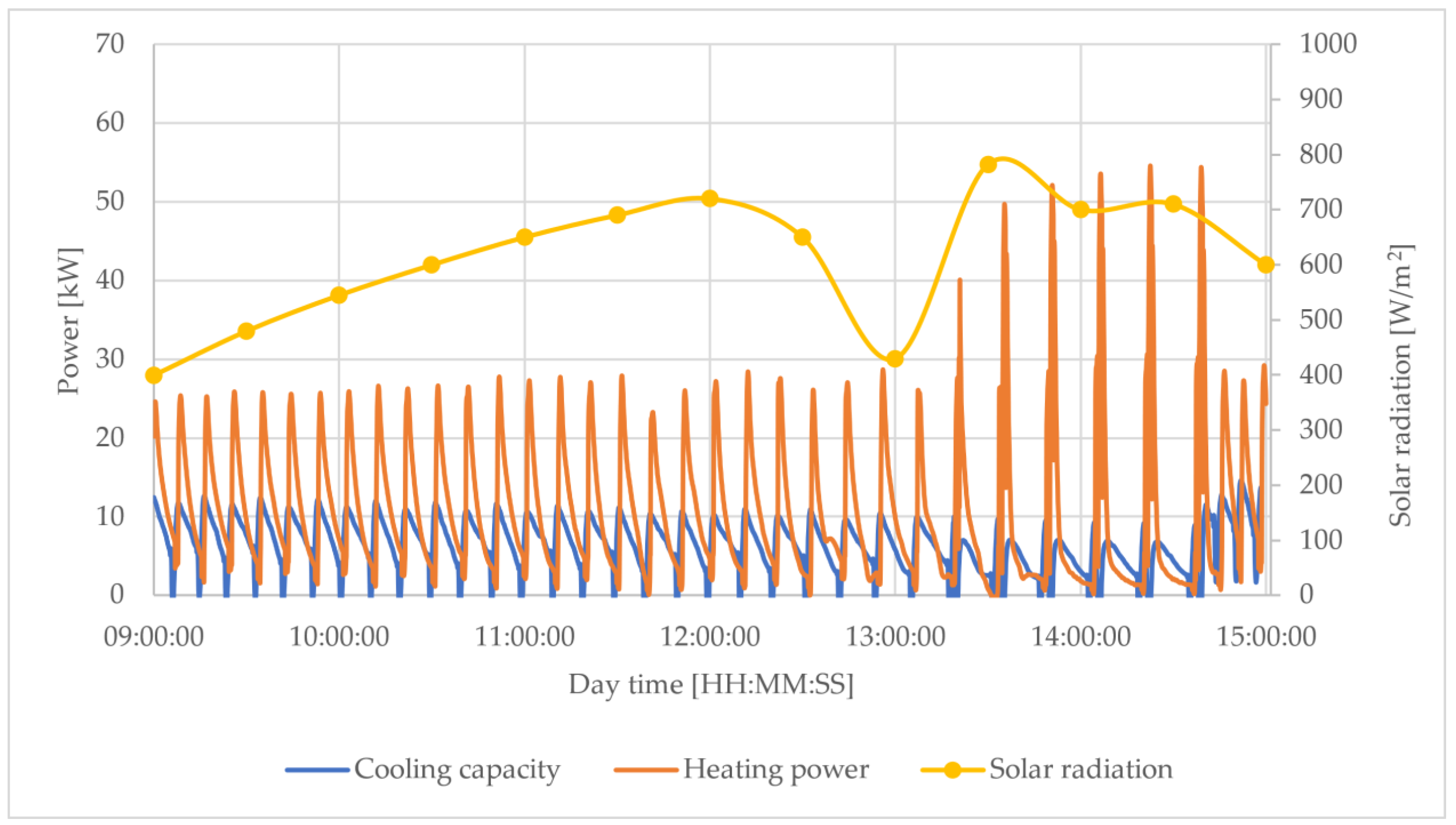
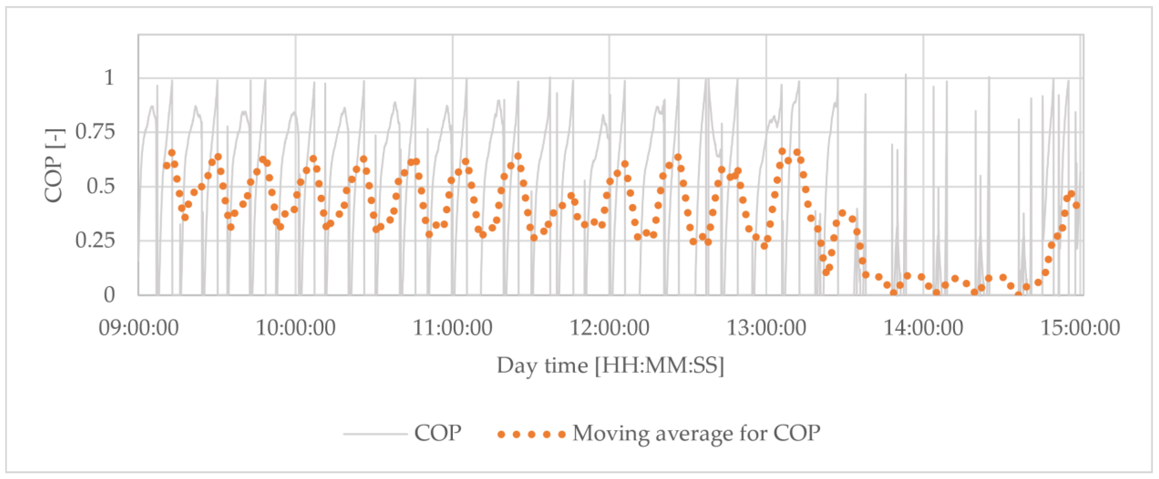
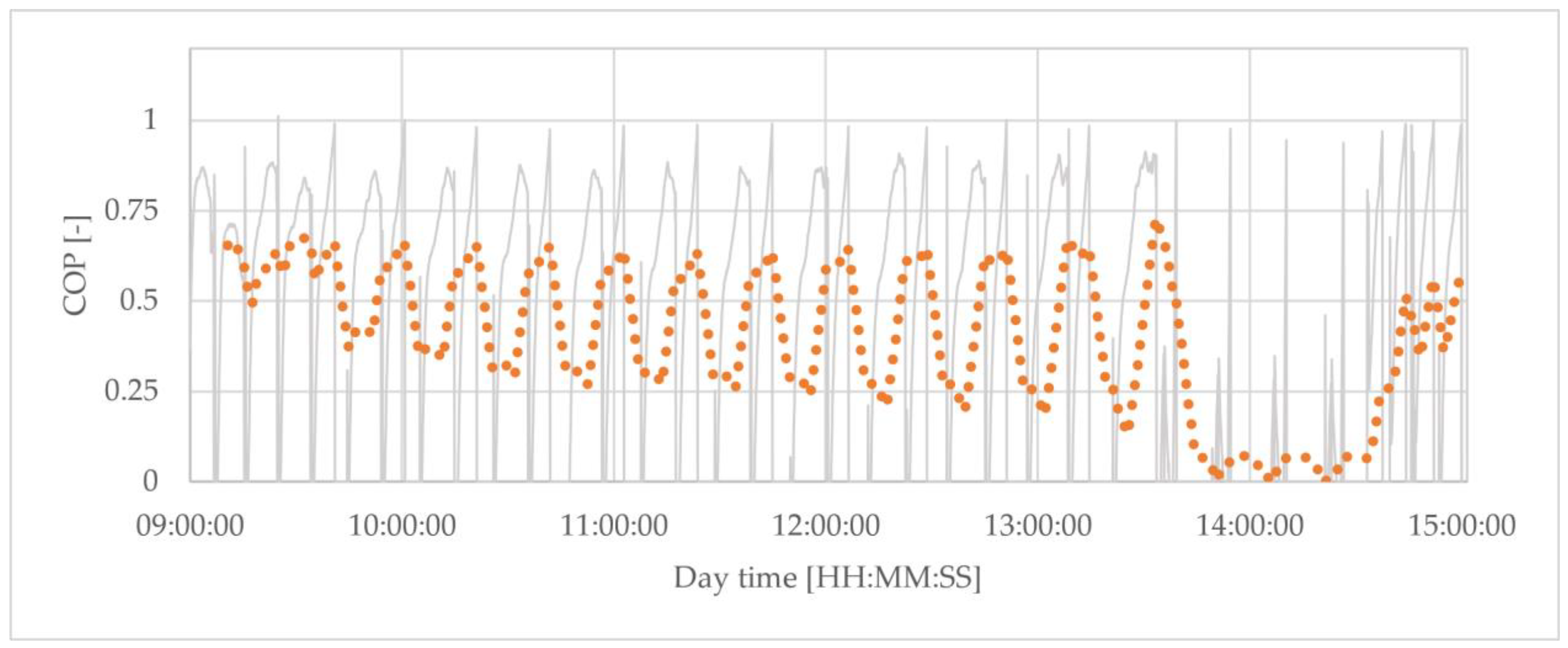
3.1. Measurements for Non-Standard Modes of Chiller Operation for July

For selected time intervals (9 a.m. to 3 p.m.), graphs of changes in water mass flow rates in the heating and chilled water circuits were drawn up for each day. In addition, the temperature parameters of the hot and chilled water were presented (Figures 9 and 12). In addition, the COP (Figures 11 and 14) and the heating power demand and chilled water production during the time under consideration were calculated from the measurements as shown in Figures 10 and 13.

When analysing the data in Figure 9, it should be concluded that the chilled water flow rate is approximately constant at 0.474 kg/s, with possible fluctuations of the order of 10⁻³ kg/s. The periodic, sudden and short increases and decreases in the flow rate are related to the switching of the chiller cycles. The hot water flow rate, in turn, remains at 0.512 kg/s and is subject to cyclic fluctuations of approx. 0.3 kg/s, which, as in the case of chilled water, is related to the cycling of the adsorption chiller operation. It should be noted that the hot water flow rate between 12 noon and 1 p.m. deviates significantly from that observed during the other hours of operation and does not resemble that recorded for 22nd July. Figure 9 also shows the course of temperature variations over time. The hot water supply temperature is 60 °C at 9 o’clock and then rises to reach a maximum of approx. 70 °C. The change in hot water outlet temperature is much more dynamic. The rapid rises and falls in temperature values over a short period of time are linked to changes in the operating phases of the unit. The greatest heat uptake takes place in the pre-heating of the bed and at the start of the desorption process, which involves a large temperature gradient and increases the heat uptake from the heating water, resulting in a difference of approx. 10 °C between the supply and return. Then, as the desorption process continues, the temperature gradient decreases, resulting in less heat being extracted from the heating water, which translates into a 2–3 °C difference between the supply and return temperatures. It is this cyclic nature of the operation that influences the shape of the hot water return temperature curve.

When analysing diagrams 9 and 10, they can be divided into three parts. The first part of the graph is the operation of the chiller between 9 a.m. and 12 p.m. (noon), where the chiller is observed to be operating at its rated cooling capacity. It should also be added that during this time, no cooling is required for the part of the building under consideration, so the cooling is accumulated in the buffer tank. This part of the graph resembles the results recorded on 22nd July. The second part of the graph shows the operation of the chiller between 12 p.m. and 1:30 p.m. when still no cooling is required on the premises, and the water temperature in the buffer tank reaches the limit value of 8 °C. This results in the chiller operating at minimum cooling capacity and the appearance of clocking, i.e., alternate switching on and off of the unit by the automation. Then, from 1:30 p.m. onwards, the correct operation of the chiller can again be observed due to the start of the cooling of the building. A pump was switched on in the cooling system of the building resulting in heat extraction and consequently an increase in the chilled water return temperature.

Figure 10 shows the calculated values for the thermal power demand and cooling capacity of the chiller over time and the meteorological data in the form of solar irradiance during the operating hours of the system. The cooling capacity for a chilled water supply temperature of approx. 10 °C reaches a maximum of approx. 10 kW, with an increase to approx. 12.4 kW was observed from 1:30 p.m. This has to do with the increase in chilled water temperature to approx. 15 °C (Figure 9) and the heat consumption in the building so that the unit can operate at a higher output. In addition, between 12 p.m. and 1:30 p.m., there is an apparent almost double increase in heating power demand as compared with the rest of the operating period. This peak in heating power is reflected in the shape of the solar irradiance curve and the heating water temperature curve. During this time, the chiller operates in the mode of minimising cooling capacity so that a very brief increase in heating power is observed, followed by a drop to zero, which is linked to the clocking of the device that is observed at chilled water temperatures below 8 °C. It should also be added that a decrease in solar irradiance between 9 a.m. and 10 a.m. does not have any negative effect on the temperature changes or the heating water flow rate. This indicates that the chiller operates correctly even during spells of cloudy weather. Figure 11 shows the instantaneous and averaged values of the COP of the chiller for operation on 8th July. The shape of the curve shows the dynamics of the process and is a direct result of the cyclic operation of the device. The COP reaches its minimum values with the start of the desorption process. At this point, the most intensive heat exchange between the hot water and the bed takes place. This is the so-called bed pre-heating phase during which the temperature difference between the inlet and outlet of the heat exchanger in the bed is the greatest. This is due to the fact that during adsorption, the temperature inside the adsorbent bed is much lower than the temperature required in the desorption phase. This difference decreases as the bed is heated, so the cooling of the water becomes less and less intense. In Figure 8, it can also be observed that between 12 p.m. and 13:3 p.m., the device is operating in the cooling capacity minimisation mode, as illustrated by a COP value close to 0. During other operating periods, the COP value fluctuates around 0.5.

Figure 12, Figure 13 and Figure 14 show the test results for 31st July. When analysing the data in Figure 12, it should be noted that the chilled water flow rate is approximately constant at 0.470 kg/s with possible fluctuations of the order of 10⁻³ kg/s. The periodic, sudden and short increases and decreases in the flow rate are related to the switching of the chiller cycles. The hot water flow rate, in turn, remains at 0.500 kg/s and is subject to cyclical fluctuations of approx. 0.40 kg/s, which, as in the case of chilled water, is related to the cycling of the adsorption chiller operation. However, the heating water flow is much more irregular than on 22nd July. The hot water supply and return temperature values do not fluctuate significantly. Likewise, the chilled water parameters are not subject to major fluctuations during the period of operation of the chiller. Nevertheless, it should be noted that the average supply temperature of chilled water is approx. 9 °C, and its return temperature is approx. 7 °C. This is an important observation with regard to the analysis of variations in the heating and cooling capacity (Figure 13) and in the COP (Figure 14). Figure 12, Figure 13 and Figure 14 can be divided into two parts, as no cooling of the building was required between 30th July and 10th August because of the holiday period. Between 9 a.m. and 10:30 a.m., normal operation of the chiller is observed, with rated cooling power and COP values. At 10:30 a.m., the temperature of the chilled water in the buffer tank reached 8 °C, and from this point onwards, the operating mode of minimising cooling capacity is observed where the device extends the cycle time in order to reduce the temperature of the water in the tank below the limit value characteristic of the chiller under consideration.

Figure 13 shows variations in the calculated values of the heating and cooling power demand and the meteorological data in the form of solar irradiance during the operating hours of the system. The cooling capacity for a chilled water supply temperature of approx. 9 °C reaches a maximum of approx. 5.8 kW and is stable over time. Attention should also be paid to the variations in the value of thermal power demand, which reaches a maximum of approx. 20 kW between 9 a.m. and 10.30 a.m., and after 10.30 a.m., the maximum value is approx. 40 kW. This is a direct result of the fact that the operation of the unit after 10:30 a.m. is abnormal, and high values of heating power are only observed momentarily and are followed by a drop in the heating power to zero. This inefficient operation is due to the lack of cooling of the building and the limited capacity of the chilled water tank.

In the same manner, as for the previous days, Figure 14 shows variations in the COP values over time for 31st July. A decrease in the efficiency of cooling production is observed after 11 a.m., which is related to the decrease in chilled water temperature and the decrease in cooling production observed in Figure 13. The average COP values observed after 10:30 a.m. confirm the observation that during this period, the chiller is operating incorrectly, minimising the cooling capacity.

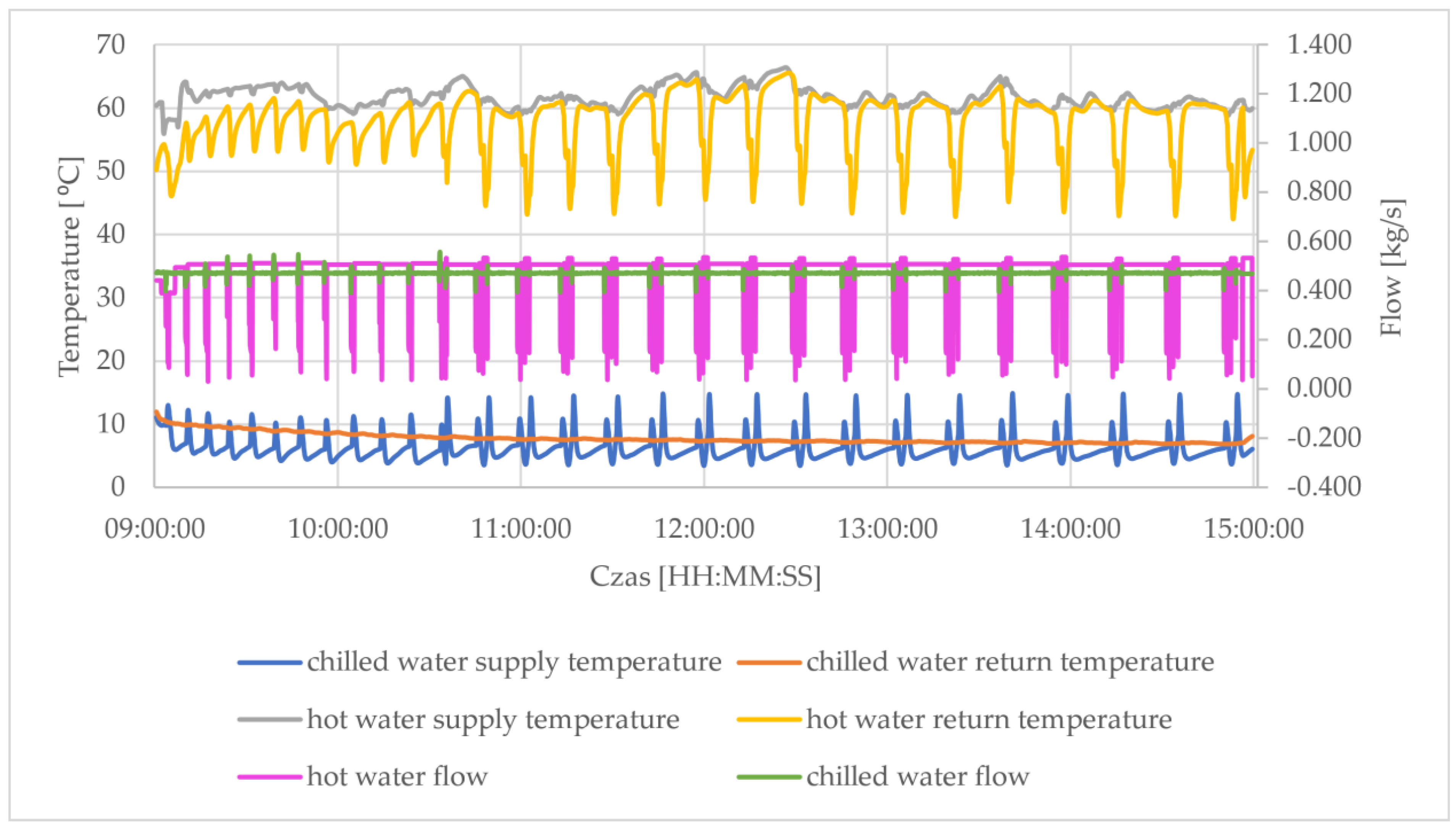
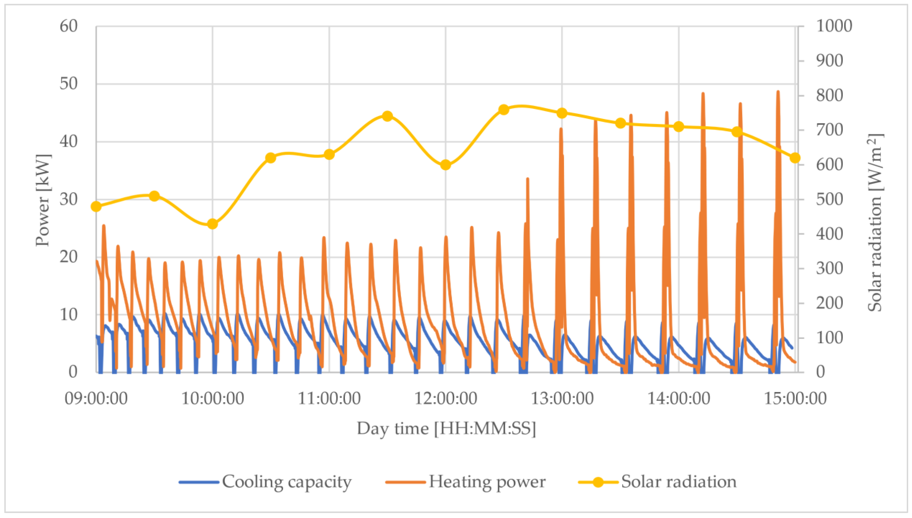
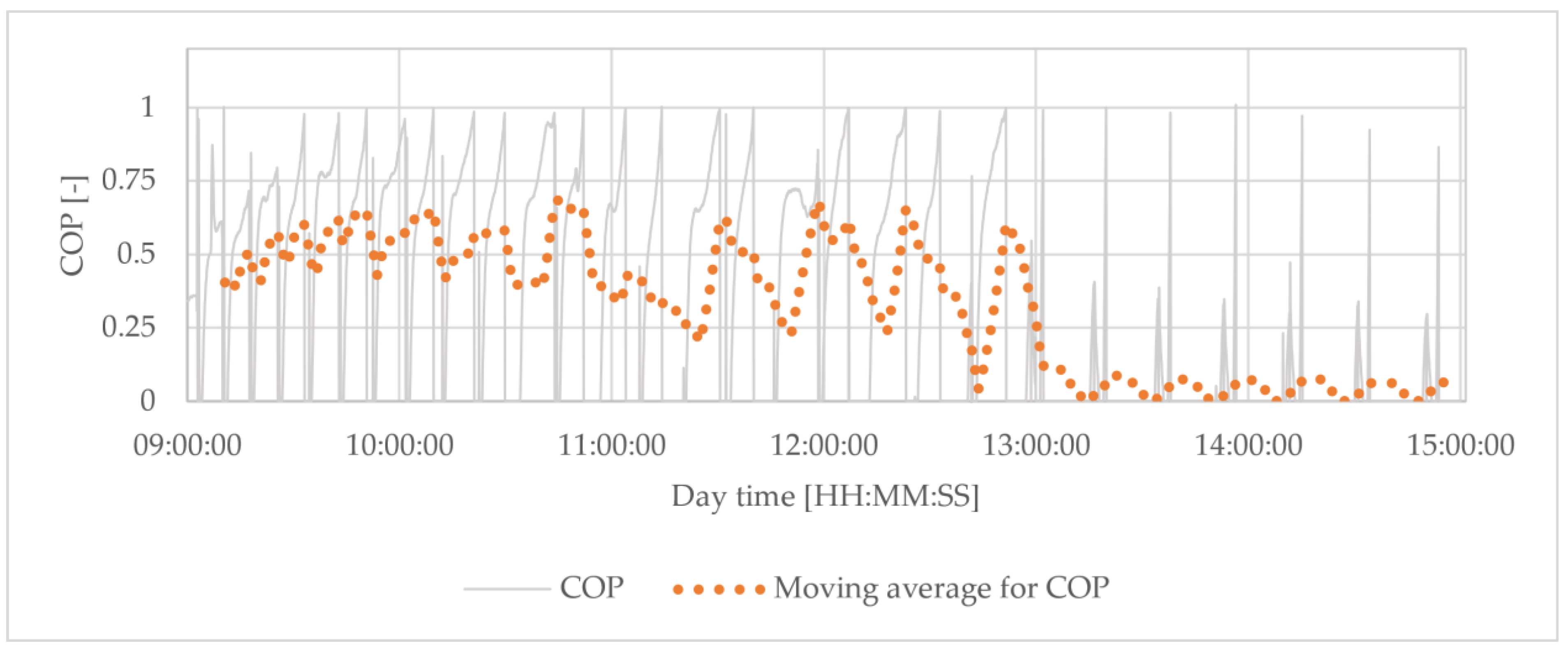
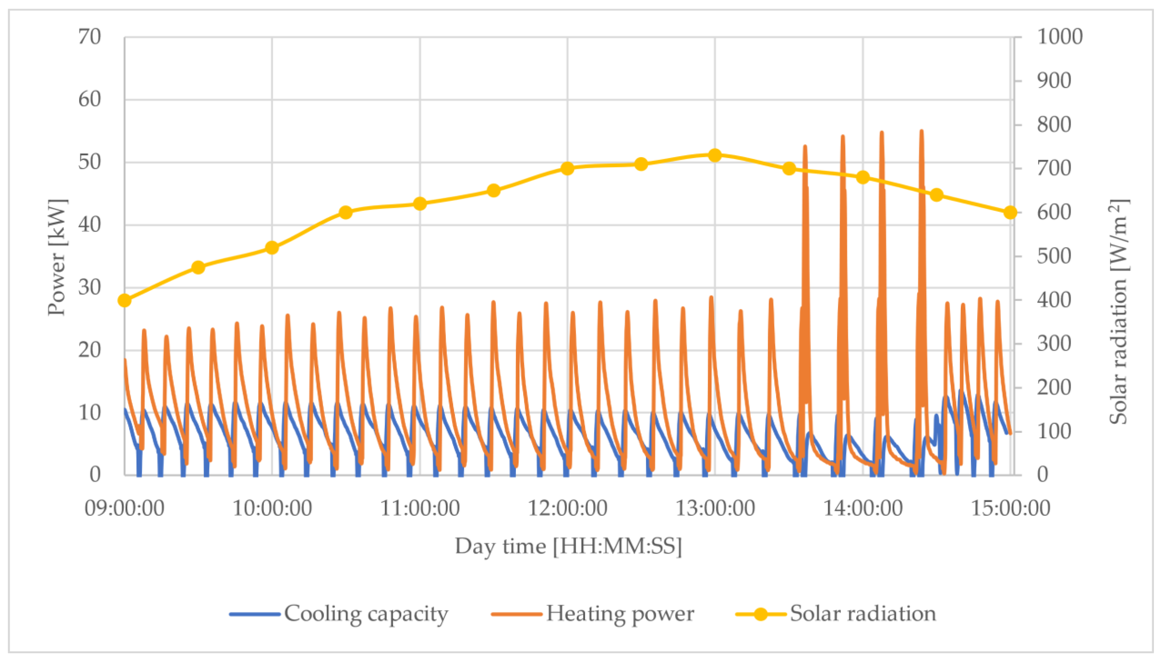
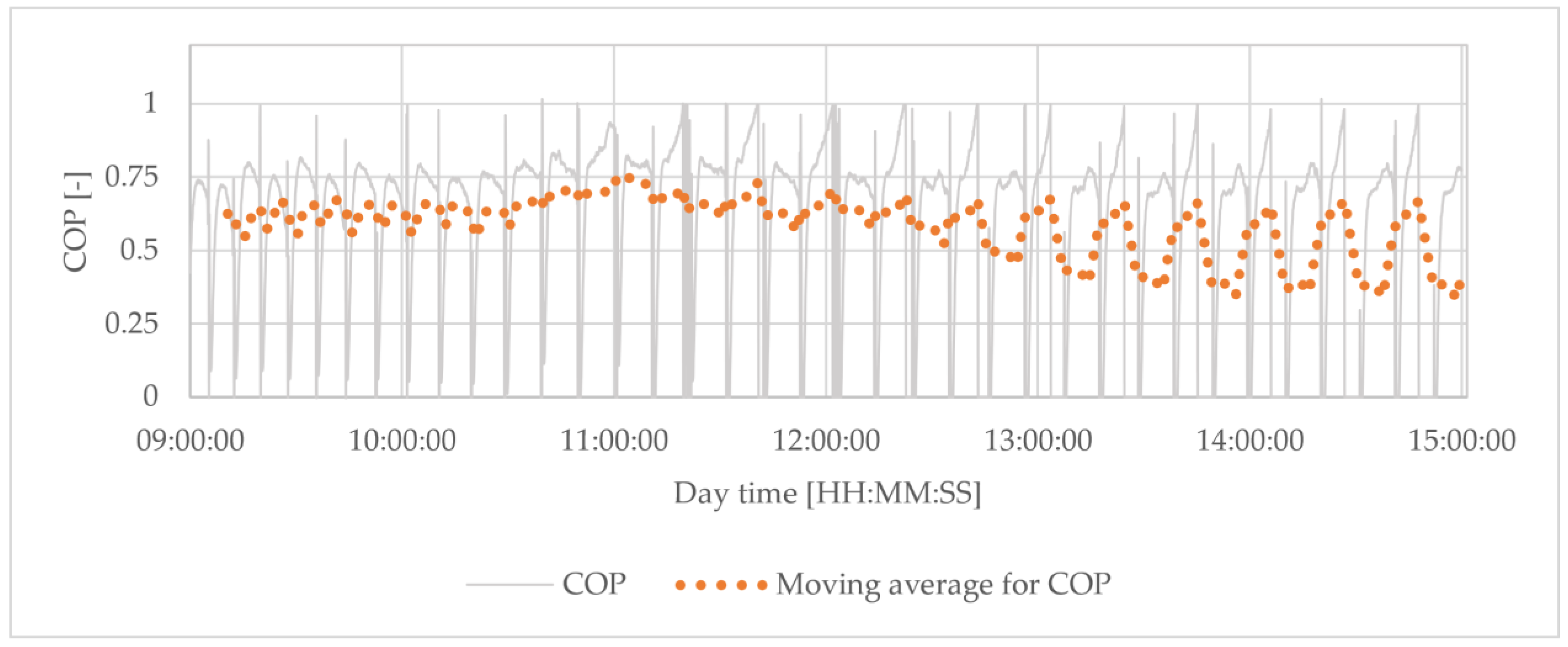
3.2. Measurements for Non-Standard Modes of Chiller Operation for August

For the selected time intervals (9 a.m. to 3 p.m.), graphs of variations in water mass flow in the heating and chilled water circuits were drawn up for each day under consideration. In addition, the temperature parameters of the hot and chilled water are presented (Figures 15, 18 and 21). In addition, the COP was calculated from the measurements (Figures 17, 20 and 23), as well as the heating power demand and cooling production during the time considered, as shown in Figures 16, 19 and 22.

Figure 15, Figure 16 and Figure 17 show the test results for 6th August. When analysing the data in Figure 15, it should be noted that the chilled water flow rate is approximately constant at 0.47 kg/s with possible fluctuations of the order of 10⁻³ kg/s. The periodic, sudden and short increases and decreases in the flow rate are related to the switching of the chiller cycles. The hot water flow rate, in turn, remains at 0.45 kg/s until 11 o’clock and then fluctuates around 0.52 kg/s and is subject to cyclical fluctuations of about 0.35 kg/s, which, as in the case of chilled water, is related to the cycling of the adsorption chiller operation. The hot water supply temperature is approx. 55 °C in the morning and reaches approx. 70 °C in the afternoon. In addition, a reduction in the chilled water supply and return temperatures are observed over time, reaching 8 °C at about 12:40 p.m. The day being conceded, i.e., 6th August, similarly to 31st July, includes the operation of the chiller during the holiday period when the cooling system in the building is switched off. Therefore, Figure 15, Figure 16 and Figure 17 can also be divided into two parts. The first part of the graph covers the operation of the chiller between 9 a.m. and 12.40 p.m. when the chiller operates at rated values of the cooling capacity and the COP. Then, when the chilled water reaches 8 °C, the chiller, as on 31st July, starts to operate in a mode involving minimisation of the cooling power, which can be seen in the form of sudden and short changes in temperature values and flow rates (Figure 15). In Figure 16, this operation can be seen in the form of very short peaks in heating power demand, which exceed 40 kW only to approach zero after a while.

Figure 17 also shows variations in the COP value over time. The curve depicted has a similar shape as the one for 31st July, i.e., after 12:40 p.m., the average COP value starts to decrease because of an apparent significant increase in the heating power demand and a reduction in the cooling capacity. This clearly indicates an abnormal operation of the chiller. Between 9 a.m. and 12:40 p.m., the chiller operates at the rated COP value that fluctuates around 0.6 and decreases slightly over time because of the decrease in the chilled water temperature.

Figure 18, Figure 19 and Figure 20 show the results of the tests for 11th August. When analysing the data in Figure 18, it should be noted that the chilled water flow rate is maintained at 0.46 kg/s with possible fluctuations in the order of 10⁻³ kg/s. The periodic, sudden and short increases and decreases in the flow rate are related to the switching of the chiller cycles. The hot water flow, in turn, fluctuates around a value of 0.52 kg/s and is subject to cyclical fluctuations of approx. 0.35 kg/s, i.e., similarly as on 6th August. The hot water supply temperature is approx. 62 °C in the morning and reaches approx. 73 °C in the afternoon. In addition, a decrease in the chilled water supply and return temperatures is observed during the time until 2:40 p.m., and then there is an increase in the chilled water return temperature of the system, which is caused by the activation of the cooling consumption in the building. Figure 18, Figure 19 and Figure 20 can be divided into three zones, as in the case of 8th August. From 9 a.m. to 1:20 p.m., the chiller operates at the rated parameters, then the chilled water temperature reaches 8 °C, and the chiller starts to operate abnormally until 2:40 p.m. From this time, the pump in the pipeline of the cooling system in the building is switched on, which is reflected by the sudden increase in the chilled water return temperature.

When analysing the data presented in Figure 19, it should be concluded that on 11th August, the solar irradiance was approximately constant and did not significantly affect the observed changes in heating power. The sudden and abrupt changes in the heating power demand and cooling capacity between 1:20 p.m. and 2:40 p.m. are caused by the fact that the chiller operates in the mode of minimising cooling capacity, which in turn is caused by a lack of cooling consumption.

Like for the days considered previously, also for 11th August, the changes in the chilled water parameters and the amount of heat used in the system are reflected in the changes in the instantaneous and averaged values of the COP. At about 1.40 p.m., the effect of the lack of cooling consumption on the operation of the chiller can be observed as the COP fluctuates around 0 during this period. Outside this period, the chiller operates efficiently, with an average COP fluctuating around 0.6.

Figure 21, Figure 22 and Figure 23 show the test results for 21st August. When analysing the data in Figure 21, it should be concluded that the chilled water flow rate remains at the same level as on the previous days. The hot water supply rate, in turn, fluctuates around a value of 0.52 kg/s and is subject to cyclic fluctuations at a level of approx. 0.35 kg/s, i.e., similar to that on 6th and 11th August. The hot water supply temperature is approx. 52 °C in the morning and reaches approx. 72 °C in the afternoon. In addition, a reduction in the chilled water supply and return temperatures is observed until 2.30 p.m., and then there is an increase in the chilled water return temperature in the system, which is the result of the start of cooling in the building. The results for 21st August are similar to those for 11th August as they cover the same periods of operation, i.e., operation outside the holiday season where building cooling is required. Between 1.30 p.m. and 2.30 p.m., the chiller operates in the undesirable mode of minimising the cooling capacity, and during the other periods, the chiller is observed to operate at rated conditions.

When analysing the solar irradiance curve for 21st August (Figure 22), it should be added that it was a cloudless day with a peak in solar irradiance occurring at 1 p.m. This curve is reflected in the hot water supply temperature curve, which is also parabolic shaped and reaches its maximum temperature value soon after 1 p.m. When analysing Figure 21 and Figure 22, it is also possible to observe a shift in the time of the solar supply peak and the cooling demand of the building, which occurs due to the thermal inertia of buildings. Consequently, the cooling of the building is only required from 2.30 p.m. On 21st August, it is observed that the chiller operates in the mode of minimising the cooling capacity between 1.30 p.m. and 2.30 p.m., where the chilled water temperature drops below 8 °C, and the chiller starts to operate abnormally.

The variations in the COP value on 21st August are almost identical to those for 11th August. Again, a decrease in the COP value is observed after 1:30 p.m., i.e., when the chiller is observed to be operating outside the rated range (chilled water temperature reaches values below 8 °C).

4. Discussion

When analysing the results of the measurements presented in this paper for the 6 days of operation of the adsorption chiller, attention should first be paid to the complexity of the system under investigation and the chiller itself and to the multiplicity of different parameters that can ultimately affect the test results. The operation of the adsorption chiller together with solar collectors is stabilised by means of buffer tanks; nevertheless, sudden changes in the intensity of solar radiation and the limited capacity of the buffer tanks are reflected in the recorded parameters of the chiller operation (e.g., switching of the chiller into the operating mode that minimises the cooling capacity). From an analysis of the graphs presented, it can be stated that it is the hot water flow rate that varies to the largest extent. However, all graphs show similar fluctuations in the hot water flow rate over the entire time period analysed. Furthermore, rapid variations in the water flow rates in the different circuits occur at the same time, which is related to the successive cycles of the chiller operation.

An analysis of the graphs above leads to the conclusion that within one cycle of the chiller operation, the instantaneous cooling capacity increases rapidly until it reaches a maximum value. Then its value decreases in an essentially linear fashion, which may be due to the fact that the chilled water production is progressively less intensive. After the cooling capacity drops to a certain value, it continues to decrease abruptly. These abrupt parameter changes in the graphs, visible as steep peaks, are associated with the switching of the processes that take place in the unit. It should be noted that the occurrence of sudden drops is observed each time in the same time periods as the mass flow spikes in the supply circuit and the chilled water circuit. The same pattern of changes in the respective temperatures and flow rates is observed for all the days under consideration. The instantaneous cooling capacity of the unit depends largely on the instantaneous values of temperature difference of the chilled water and less on the magnitude of the flows in the chilled water, cooling water and hot water circuits. It should also be concluded that for each of the days considered, the chilled water supply and return temperatures decrease along with the duration of the chiller operation. For 31st July and 6th August, the chilled water temperature is reduced to 8 °C, and then the unit starts to operate in chiller capacity minimisation mode because of the lack of cooling consumption in the building (holiday season and periods when no cooling is required). On 22nd July, the chiller operates at rated parameters, with 24 h cooling consumption. On 8th July, 11th August and 21st August, the chiller operates at rated parameters before noon; then, depending on the day, from about 12 p.m. to 1.30 p.m., it starts to operate in a mode of minimising cooling capacity due to the lack of cooling consumption. From about 1:30 p.m., the chiller starts to operate again at rated parameters as the building starts to consume cooling. It is for this reason that at about 1:30 p.m., the chilled water return temperature suddenly rises, which is the result of the start-up of the cooling system in the building. Another observation relating to the return temperature curve in the chilled water circuit is that each time this temperature falls below 8 °C, the heating energy requirement doubles, and the cooling capacity of the unit decreases. These results are directly related to the performance potential of the device. The chiller in the investigation is capable of producing chilled water at a minimum temperature of 8 °C, and as soon as this temperature is reached in the buffer tank, the unit starts to operate in capacity minimisation mode. The control system extends the cycle time in order to lower the pressure in the evaporator and thus continue to lower the chilled water temperature, but this is beyond the capacity of the unit. This is due to the built-in algorithm that protects the adsorption bed from overcooling where the chiller is temporarily shut down when the chilled water supply temperature reaches 4 °C. Consequently, during the periods analysed, the chiller operates in a kind of ‘on-off’ standby mode, resulting in sudden and short changes in temperature, heating power and cooling capacity with a COP close to 0.

Table 4. Summary of basic system operating parameters for the days considered.

Date	Average Solar Radiation [W/m2]	Average Cooling Capacity [kW]	Average Heating Power [kW]	Average COP [-]	Average Hot Water Temperature [°C]	Average Chilled Water Flow [kg/s]	Average Chilled Water Temperature [°C]
8th July	424.1	7.18	13.36	0.605	61.7	0.474	11.7
22nd July	718.9	8.71	13.32	0.677	57.7	0.471	12.5
31st July	647.0	5.16	14.27	0.400	60.2	0.471	8.6
6th August	642.8	6.79	13.54	0.584	62.0	0.473	8.1
11th August	621.4	7.83	15.19	0.584	67.6	0.475	12.7
21st August	627.2	7.53	14.00	0.582	62.5	0.478	11.1

presents a summary of the basic operating parameters of the chiller obtained by integrating the relevant curves in the graphs. When analysing these data, it should be borne in mind that the entire system operates using buffer tanks, so each temperature and its variations also depend on the temperature prevailing in the tanks at the beginning of a particular day and the variations in the solar irradiance during the day. The manufacturer’s rated cooling capacity values refer to a selection of three operating points, where the heating water temperature is 65 °C or 85 °C. It is, therefore, difficult to find points of reference between the rated data and the test results. Based on the values compiled in Table 4, it can be concluded that lowering the chilled water temperature results in a decrease in the COP value. By analysing the average COP values shown, a correlation can be seen between the COP value and the duration of irregular chiller operation. Obviously, the lowest average COP was calculated for 31st July when the chiller was already operating in ‘on-off’ mode from 10:30 a.m. (but this is not the normal operating mode of the device). On 22nd July, on the other hand, the instantaneous operation of the chiller is observed with an average COP of 0.677, which is above the maximum value stated by the manufacturer. Nevertheless, this can be explained by the relatively high chilled water temperature of 12.5 °C and the stable operation of the chiller, which is due, among other things, to the high and stable solar irradiance on that day; the operation is regular throughout the operating period.

When relating the results to other published papers, it should be stated that the adsorption chiller combined with a solar collector system and operating under Polish climatic conditions does not differ from systems located in the Middle East or South Europe in terms of achieved cooling power and COP efficiency. Hassan et al. [38] analysed the performance of an adsorption chiller operating with PVT solar panels in the regions of the Middle East and North Africa. The results for July show that the maximum cooling capacity and the COP are approx. 7.44 kW and 0.42 for Alexandria, 8.1 kW and 0.43 for Dubai, and 7.439 kW and 0.42 in Riyadh, respectively. Angrisani et al. [39] analysed the interoperation between an adsorption chiller and flat-plate and solar vacuum collectors in southern Italy. The authors obtained average COP results in the range of 0.43–0.45 and a cooling capacity of 10 kW. It should also be added that a system with flat-plate collectors requires 4.5 m² of collector area per 1 kW of power, while a system with vacuum collectors requires 3.1 m²/kW. This is important information with regard to the limited area for the installation of collectors. Based on the above results reported by other authors, it can be concluded that no major differences are observed between the operation of a solar adsorption chiller under warm and temperate climate conditions in terms of the chiller performance achieved. The only difference is the amount of solar irradiance, which is lower in Poland than in Italy or the Middle East, but this also translates into lower cooling requirements for buildings. On the other hand, attention should be paid to the difficulty of integrating an adsorption chiller into building cooling systems. In this paper, the operation of the chiller was analysed during periods of standard building use and during holiday periods when the cooling was switched off. Irregular and inefficient operation of the chiller was observed on days when there was no heat transfer (cooling capacity minimisation and chiller protection mode). The chilled water buffer tank with a capacity of 5 m³ proved to be insufficient, which forced the chiller to operate in the on–off mode, which is selected at low COP values. From the perspective of energy consumption, this is, therefore, a disadvantage, but it protects the unit from damage. It is worth mentioning here that the heating energy supplied to the system during this time must be discharged into the environment. In addition, due to the nature of the building and its location, cooling is required more or less after 1 p.m. so that even on days of standard use of the building, the on–off operation could not be avoided. Therefore, consideration should be given to reconfiguring the system to avoid intermittent operation at times of no cooling consumption, e.g., by increasing the capacity of the cooling buffer, which should allow the chiller to run for longer at rated conditions.

Nevertheless, it has to be stated systems consisting of solar thermal collectors and solar adsorption chillers can provide an alternative to the traditional air-conditioning systems, and further work on these systems and on heat storage for chillers, whether in the form of the selection of hot water buffers or storage in the form of phase-change materials, is justified. The increasing use of renewable energy sources in buildings also generates problems, some of which have been highlighted in this paper, so the limitations mentioned above, which arise from the cyclic and weather-dependent operation of such systems, must also be borne in mind.

5. Conclusions

This paper analyses the operation of a solar adsorption chiller under climatic conditions characteristic of Central and Eastern Europe. Exactly the location of the analysed installation in Poland is extremely important from the point of view of the usefulness of the obtained results. Climatic conditions in Poland are characteristic of much of Europe, which allows the results obtained to be used by a wide group of people. Based on the results obtained during experimental tests on an actual system, it was found that:

(1)

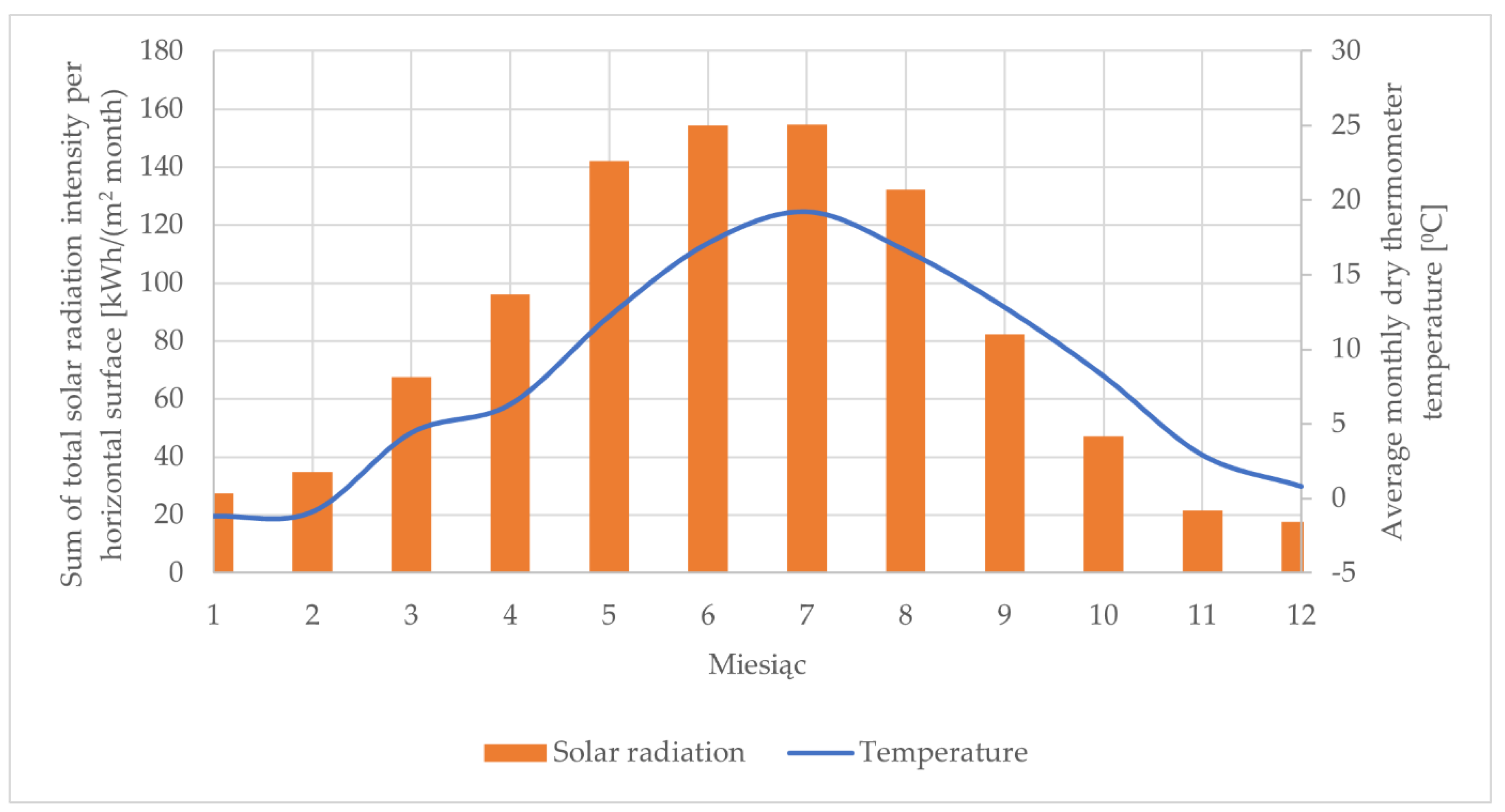
It is possible to use a solar thermal system to power an adsorption cooling system for solar radiation conditions characteristic of Central and Eastern European regions;

(2)

As the chilled water temperature decreases, the values of the cooling capacity of the unit and of the COP decrease;

(3)

Variations in solar irradiance during the day and changes in the cooling capacity can be effectively compensated for by heating and chilled water buffer tanks;

(4)

At the time of testing, the average COP was 0.400 ÷ 0.677, the average cooling capacity was 5.16 ÷ 8.71 kW, the average solar irradiance was 424.1 ÷ 718.9 W/m², the average heating power demand was 13.32 ÷ 15.19 kW, and the average heating water supply temperature was 57.7 ÷ 67.2 °C.

Based on the investigation and analysis of the results, it should be concluded that the adsorption chillers available on the market can be successfully applied under the climatic conditions characteristic of the Polish region, and it is possible to operate such systems at the nominal parameters of cooling power and COP efficiency. However, the following aspects should be noted with regard to the application of adsorption refrigeration systems integrated with the systems of solar thermal collectors:

(1)

A long time is needed to ensure stable operation as compared with compressor chillers.

(2)

Chillers of this type have a small range of cooling capacity adjustment, i.e., 60–100%.

(3)

An additional heat discharge system is required to prevent the system from overheating if there is no cooling production. Such a situation was just observed in the case under review, where the cooling of the scientific and research centre is irregular due to the varying intensity of use of the facility. A similar situation is observed in public administration buildings, where cooling is also not required during the weekend period.

(4)

The highest heat production from solar thermal installations occurs in this type of building, mainly during the holiday season when there is usually a reduction in cooling demand due to reduced intensity building use.

When designing adsorption refrigeration systems integrated with a solar thermal system, attention must be paid to the appropriate selection of thermal and cold storage capacities to ensure stable operation of the adsorption chiller and the possibility of discharging high-temperature and medium-temperature heat (in the investigation, the discharged was to outdoor air and the ground).

The growth of the refrigeration and air-conditioning sector mentioned in the introduction and the consequently increasing consumption of electricity draw attention to the need for research within the framework of implementing a circular economy and sustainable development. A topic for future studies might also be an analysis of the selection of the number and location of solar collectors and the capacity of buffer tanks for selected buildings in terms of providing desorption heat for the adsorption chiller and providing domestic hot water or seasonal heat storage in the ground. Such a system would enable the operation of buildings during the summer period based on renewable energy sources with minimum electricity consumption and provision of heat for heating during the winter period using a heat pump.

In addition, it is important to note another aspect that shows the importance of the research being conducted. The temperate warm transitional climate that prevails in Central and Eastern Europe influences the need to cool buildings in summer and heat them in winter. This affects the high energy consumption of buildings located in this part of Europe. This fact, in conjunction with the current situation in the market for energy resources and the European Union’s policy of electrification of the heating and district heating sector, influences the need to increase efficiency in energy use. The need to accelerate the energy transition and ensure energy security can provide further stimulation for the wider use of adsorption chillers integrated with renewable energy sources. This clearly establishes the legitimacy of the research and indicates the need for further studies on this topic.

References

- Birol, F. The Future of Cooling: Opportunities for Energy-Efficient Air Conditioning; Report of the International Energy Agency, International Energy Agency: Paris, France, 2018; Available online: https://www.iea.org/reports/the-future-of-cooling (accessed on 12 July 2022).
- Dupont, J.L.; Domanski, P.; Lebrun, P.; Ziegler, F. The Role of Refrigeration in the Global Economy (2019), 38th Note on Refrigeration Technologies; Informatory note of the International Institute of Refrigeration; The International Institute of Refrigeration: Paris, France, 2019. [Google Scholar]
- Papakokkinos, G.; Castro, J.; Capdevila, R.; Damle, R. A Comprehensive Simulation Tool for Adsorption-Based Solar-Cooled Buildings—Control Strategy Based on Variable Cycle Duration. Energy Build. 2021, 231, 110591. [Google Scholar] [CrossRef]
- Key World Energy Statistics 2021; Report of the International Energy Agency; International Energy Agency: Paris, France, August 2021. Available online: https://www.iea.org/reports/key-world-energy-statistics-2021 (accessed on 12 July 2022).
- Cooling; Report of the International Energy Agency; International Energy Agency, Paris, France. 2021. Available online: https://www.iea.org/reports/cooling (accessed on 12 July 2022).
- Wang, L.; Bu, X.; Ma, W. Experimental study of an Adsorption Refrigeration Test Unit. Energy Procedia 2018, 152, 895–903. [Google Scholar] [CrossRef]
- Zajaczkowski, B. Optimizing performance of a three-bed adsorption chiller using new cycle time allocation and mass recovery. Appl. Therm. Eng. 2016, 100, 744–752. [Google Scholar] [CrossRef]
- Ng, K.C.; Thu, K.; Kim, Y.; Chakraborty, A.; Amy, G. Adsorption desalination: An emerging low-cost thermal desalination method. Desalination 2013, 308, 161–179. [Google Scholar] [CrossRef]
- Pan, Q.; Peng, J.; Wang, R. Experimental study of an adsorption chiller for extra low temperature waste heat utilization. Appl. Therm. Eng. 2019, 163, 114341. [Google Scholar] [CrossRef]
- Sztekler, K.; Kalawa, W.; Mika, L.; Krzywanski, J.; Grabowska, K.; Sosnowski, M.; Nowak, W.; Siwek, T.; Bieniek, A. Modeling of a Combined Cycle Gas Turbine Integrated with an Adsorption Chiller. Energies 2020, 13, 515. [Google Scholar] [CrossRef]
- Krzywanski, J.; Sztekler, K.; Bugaj, M.; Kalawa, W.; Grabowska, K.; Chaja, P.R.; Sosnowski, M.; Nowak, W.; Mika, Ł.; Bykuć, S. Adsorption chiller in a combined heating and cooling system: Simulation and optimization by neural networks. Bull. Pol. Acad. Sci. Tech. Sci. 2021, 69, e137054. [Google Scholar]
- Scopus Database. Available online: https://www.scopus.com/search/form.uri?display=basic#basic (accessed on 12 July 2022).
- Fan, Y.; Luo, L.; Souyri, B. Review of solar sorption refrigeration technologies: Development and applications. Renew. Sustain. Energy Rev. 2007, 11, 1758–1775. [Google Scholar] [CrossRef]
- Younes, M.M.; El-Sharkawy, I.I.; Kabeel, A.E.; Saha, B.B. A review on adsorbent-adsorbate pairs for cooling applications. Appl. Therm. Eng. 2017, 114, 394–414. [Google Scholar] [CrossRef]
- Choudhury, B.; Saha, B.B.; Chatterjee, P.K.; Sarkar, J.P. An overview of developments in adsorption refrigeration systems towards a sustainable way of cooling. Appl. Energy 2013, 104, 554–567. [Google Scholar] [CrossRef]
- Wang, D.C.; Li, Y.H.; Li, D.; Xia, Y.Z.; Zhang, J.P. A review on adsorption refrigeration technology and adsorption deterioration in physical adsorption systems. Renew. Sustain. Energy Rev. 2010, 14, 344–353. [Google Scholar] [CrossRef]
- Alelyani, S.M.; Bertrand, W.K.; Zhang, Z.; Phelan, P.E. Experimental study of an evacuated tube solar adsorption cooling module and its optimal adsorbent bed design. Sol. Energy 2020, 211, 183–191. [Google Scholar] [CrossRef]
- Liu, Y.M.; Yuan, Z.X.; Wen, X.; Du, C.X. Evaluation on performance of solar adsorption cooling of silica gel and SAPO-34 zeolite. Appl. Therm. Eng. 2021, 182, 116019. [Google Scholar] [CrossRef]
- Bouzeffour, F.; Khelidj, B.; Abbes, M.T. Experimental investigation of a solar adsorption refrigeration system working with silicagel/water pair: A case study for Bou-Ismail solar data. Sol. Energy 2016, 131, 165–175. [Google Scholar] [CrossRef]
- Lattieff, F.A.; Atiya, M.A.; Al-Hemiri, A.A. Test of solar adsorption air-conditioning powered by evacuated tube collectors under the climatic conditions of Iraq. Renew. Energy 2019, 142, 20–29. [Google Scholar] [CrossRef]
- Qadir, N.U.; Said, S.A.M.; Mansour, R.B.; Imran, H.; Khan, M. Performance comparison of a two-bed solar-driven adsorption chiller with optimal fixed and adaptive cycle times using a silica gel/water working pair. Renew. Energy 2020, 149, 1000–1017. [Google Scholar] [CrossRef]
- Pan, Q.W.; Wang, R.Z. Study on operation strategy of a silica gel-water adsorption chiller in solar cooling application. Sol. Energy 2018, 172, 24–31. [Google Scholar] [CrossRef]
- Rouf, R.A.; Amanul, K.C.A.; Saha, B.B.; Kabir, K.M.A. Utilizing Accessible Heat Enhancing Cooling Effect with Three Bed Solar Adsorption Chiller. Heat. Transf. Eng. 2019, 40, 1049–1059. [Google Scholar] [CrossRef]
- Alahmer, A.; Wang, X.; Al-Rbaihat, R.; Alam, K.C.A.; Saha, B.B. Performance evaluation of a solar adsorption chiller under different climatic conditions. Appl. Energy 2016, 175, 293–304. [Google Scholar] [CrossRef]
- Jaiswal, A.K.; Mitra, S.; Dutta, P.; Srinivasan, K.; Murthy, S.S. Influence of cycle time and collector area on solar driven adsorption chillers. Sol. Energy 2016, 136, 450–459. [Google Scholar] [CrossRef]
- Halon, T.; Lukmin, P.; Szyc, M.; Bialko, B.; Zajaczkowski, B. Case study of the adsorption chiller driven by combined municipal heat and solar energy. In Proceedings of the 25th IIR International Congress of Refrigeration, Montréal, QC, Canada, 24–30 August 2019. [Google Scholar] [CrossRef]
- Alahmer, A.; Wang, X.; Alam, K.C.A. Dynamic and Economic Investigation of a Solar Thermal-Driven Two-Bed Adsorption Chiller under Perth Climatic Conditions. Energies 2020, 13, 1005. [Google Scholar] [CrossRef]
- El-Sharkawy, I.I.; AbdelMeguid, H.; Saha, B.B. Potential application of solar powered adsorption cooling systems in the Middle East. Appl. Energy 2014, 126, 235–245. [Google Scholar] [CrossRef]
- Reda, A.M.; Ali, A.H.H.; Taha, I.S.; Morsy, M.G. Performance of a small-scale solar-powered adsorption cooling system. Int. J. Green Energy 2017, 14, 75–85. [Google Scholar] [CrossRef]
- Rouf, R.A.; Jahan, N.; Alam, K.C.A.; Sultan, A.A.; Saha, B.B.; Saha, S.C. Improved cooling capacity of a solar heat driven adsorption chiller. Case Stud. Therm. Eng. 2020, 17, 100568. [Google Scholar] [CrossRef]
- Chen, Q.F.; Du, S.W.; Yuan, Z.X.; Sun, T.B.; Li, Y.X. Experimental study on performance change with time of solar adsorption refrigeration system. Appl. Therm. Eng. 2018, 138, 386–393. [Google Scholar] [CrossRef]
- Elsheniti, M.B.; Rezk, A.; Shaaban, M.; Roshdy, M.; Nagib, Y.M.; Elsamni, O.A.; Saha, B.B. Performance of a solar adsorption cooling and desalination system using aluminum fumarate and silica gel. Appl. Therm. Eng. 2021, 194, 117116. [Google Scholar] [CrossRef]
- Robbins, T.; Garimella, S. An autonomous solar driven adsorption cooling system. Sol. Energy 2020, 211, 1318–1324. [Google Scholar] [CrossRef]
- Sha, A.A.; Baiju, V. Thermodynamic analysis and performance evaluation of activated carbon-ethanol two-bed solar adsorption cooling system. Int. J. Refrig. 2021, 123, 81–90. [Google Scholar] [CrossRef]
- Fernandes, M.S.; Brites, G.J.V.N.; Costa, J.J.; Gaspar, A.R.; Costa, V.A.F. Review and future trends of solar adsorption refrigeration systems. Renew. Sustain. Energy Rev. 2014, 39, 102–123. [Google Scholar] [CrossRef]
- SorTech AG Company Materials. Operating Manual of SorTech eCoo 2.0. 13.12.2016.
- Kingspan Environmental Sp. z o.o. Company Materials. Available online: https://www.kingspan.com (accessed on 12 July 2022).
- Hassan, A.A.; Elwardany, A.E.; Ookawara, S.; El-Sharkawy, I.I. Performance investigation of integrated PVT/adsorption cooling system under the climate conditions of Middle East. Energy Rep. 2020, 6, 168–173. [Google Scholar] [CrossRef]
- Angrisani, G.; Entchev, E.; Roselli, C.; Sasso, M.; Tariello, F.; Yaïci, W. Dynamic simulation of a solar heating and cooling system for an office building located in Southern Italy. Appl. Therm. Eng. 2016, 103, 377–390. [Google Scholar] [CrossRef]