Cooling Modelling of an Electrically Heated Ceramic Heat Accumulator

Abstract

This paper presents a simple novel mathematical model of a heat accumulator with an arranged packing in the form of ceramic cylinders. The accumulator analysed in the paper can be heated with inexpensive electricity overnight or excess electricity from wind farms. It can be used as a heat source in a hydronic heating system or for domestic hot water. The differential equations describing the transient temperature of the accumulator packing and flowing air were solved using the explicit Euler and Crank–Nicolson methods. The accuracy of both methods was assessed using exact analytical solutions and the superposition method for a uniform initial temperature and accounted for time changes in inlet air temperature. A numerical simulation of the accumulator cooled by flowing air was carried out. The correlation for the air-side Nusselt number was determined using the method of least squares based on experimental data. The calculated exit air temperature was compared with the measured data. The accumulator can operate as a heat source with dynamic discharge. The developed mathematical model of the accumulator can be used in a system to adjust the fan rotational speed so that the air temperature in the room is equal to the preset temperature.

1. Introduction

In recent years, there has been increasing interest in both heat and electricity storage. This is mainly due to the time-varying power generated by renewable energy sources such as wind and photovoltaic farms. Ceramic-filled heat accumulators or electrically heated hot water storage tanks can utilise surplus electrical energy from photovoltaics and wind farms, which will improve the controllability of the entire energy system.

Water, solid materials, and phase-change materials (PCMs) are most commonly used as thermal storage materials [1]. Large water heat storage tanks with hot and cold water stratification are widely used in urban central heat supply systems. The paper [2] presents CFD modelling of a water heat accumulator with water temperature stratification used in a large municipal thermal power plant comprising coal-fired grate boilers and natural gas-fired internal combustion engines. Pressurised hot water storage tanks are also used to improve the flexibility of thermal power units. One way of managing excess electricity at night; i.e., during times of reduced electricity demand, is through the accumulation of hot water in pressurised storage tanks. The heat flow rate supplied to the power plant with the fuel is partly used during the night period to heat up the hot water in the accumulators, resulting in a reduction in the electrical power generated. The boiler in this situation can operate above the technical minimum without burning heavy fuel oil in the chamber. In the case of boilers fired with pulverised coal, when the boiler load is below the technical minimum, pulverised coal and fuel oil are burnt in the boiler simultaneously to avoid the pulverised coal burners being extinguished. Thanks to these tanks, it is possible to increase the maximum load of the power unit by a few percent and decrease the value of the minimum acceptable load of the power unit by dozens of percent [3]. A concept of a nuclear plant with improved flexibility was described in [4]. Water tanks and borehole thermal energy-storage systems (BTES) can be used for thermal energy storage for district heating systems utilising waste heat from data centres [5]. The application of water-to-water heat pumps in a solar system for space heating and domestic hot water preparation in a cold climate was presented by Pinamonti et al. [6]. A seasonal water storage tank for a single-family house was used to store the excess heat. The long-term storage tank was completely buried under the ground near the house. Electric water heaters affected the operation of the entire energy system. The flexibility potential of electric water heaters was strongly influenced by the daily hot water demand [7]. Hot water storage tanks can be used to capture the excess electricity generated by photovoltaic cells [8]. A system consisting of photovoltaic cells and an electric water heater can essentially meet a household’s electricity and heat requirements for heating a building [9]. A novel hot water storage unit with low thermal inertia was proposed for floor heating and domestic hot water preparation using solar collectors. The proposed solution ensured stable system operation even after sunset [10].

The use of a proportional water flow controller in a hot water preparation system with a hot water reservoir was presented in [11]. The effect of thermometer inertia on temperature control quality in an electrically heated hot water reservoir was investigated in [12]. The correct operation of the temperature control in the hot water storage tank was strongly influenced by random temperature measurement errors. The accidental errors in the thermometer indications could result in the faulty operation of the PID controller, since the water temperature in the tank could rise steadily despite exceeding the set temperature [13].

Solid-fill accumulators are often used for heating buildings and domestic hot water preparation. The filling of the accumulator can be either structured or random. A ceramic filling resistant to high temperatures in the order of 800 °C is used in the designed battery. As a result, a large amount of heat can be stored in the lightweight heat storage unit, which is used to heat the building. The use of fireproof ceramic cylinders in the proposed accumulator is an inexpensive and safe solution. The accumulator filling can be made of other materials; e.g., magnetite, as it has a high specific gravity and high heat capacity. In the general case, high-density, high-heat-capacity, high-temperature-resistant materials are the materials from which the filling can be made. Due to the high temperature of the accumulator packing when charged, materials such as concrete or stones are unsuitable due to their low resistance to thermal stress cracking. The ceramic elements are arranged in an orderly manner so that the porosity of the filling can be reduced and the pressure loss when air flows through the accumulator is reduced. This results in a reduction in the energy consumed by a fan pushing air through the accumulator.

A numerical model of a channel heat accumulator heated by hot air was presented in [14]. Computer simulations showed that the number of finite elements along the duct length had to be large to ensure satisfactory accuracy of the air temperature calculations at a low air velocity.

The standard approach in heat accumulator modelling, in which the average temperature of the flowing gas along the length of one cell is approximated by the arithmetic mean of the inlet and outlet temperatures of the cell, can lead to substantial errors, especially for small mass flow rates of the gas [14]. It is necessary to divide the accumulator model into a considerable number of cells; e.g., into 50 or more, to achieve a numerical solution of the system of differential equations for an accumulator that does not change with the increasing number of cells and agrees well with the experiment. This requirement applies to the finite-difference method, including both the explicit Euler method and the Crank–Nicolson method. Furthermore, in contrast to heat conduction issues, the stability and accuracy of modelling heat accumulators with different numerical methods have not been sufficiently investigated in the literature.

A hybrid finite volume method–finite element method was used to simulate the operation of the accumulator with an organised structure [15]. The results of the calculations carried out in [15] were compared with the measurements. A heat storage unit made of steel or concrete cylindrical elements was modelled using the COMSOL Multiphysics 4.3a software [16]. The operation of a honeycomb ceramic heat accumulator was simulated using a one-dimensional model in the object-oriented modeling language Modelica [17]. A simple transient floor heating model was presented in [18]. The solution of the one-dimensional transient heat conduction was solved using a Laplace transform. The storage capacity of the floor and the energy transferred from the floor to the heated space were estimated. A resistance-heated energy storage unit made of firebricks was studied in [19]. The thermal performance of the industrial heat accumulator was studied numerically using the finite volume method in conjunction with the Crank–Nicolson method. The paper [20] presented the concept of a graphite heat accumulator. The heat was accumulated in a graphite block in which steel water tubes were installed. The advantage of such an accumulator over this type of concrete accumulator was the higher operating temperature of the graphite block and lower thermal stresses in the graphite block due to the high value of the graphite thermal conductivity of about 88 W/(m·K). A combined heat and compressed air energy-storage system using a packed bed accumulator and an electrical heater was proposed in [21]. The thermal oil was resistively heated to a high temperature, stored in a reservoir, and then directed to an interstage air superheater located between the air turbine’s high- and low-pressure parts. An air-based high-temperature heat and power storage system that cogenerated heat and electricity with high efficiency was presented in [22]. During the charging process, the packed bed of stones was heated up to 685 °C. The effect of the thermal conductivity of the solid particles that made up the filling of a heat accumulator was analysed in [23].

In the last few decades, there has been a lot of research on the application of phase-change materials (PCMs) for heat storage in technical systems. Numerical modelling of the combined sensible–latent heat-storage unit with a periodic flow used in concentrated solar power plants was carried out in [24]. Solid (GF/Sn-Bi composite) and PCM (GF/MgCl₂ composite) were used in numerical simulations of the proposed solution. A significant problem in the broader use of PCM-based heat storage is the high thermal inertia. Usually, a small area close to the components to be heated or cooled; e.g., pipes or flat surfaces, is used. A large part of the tank does not undergo a phase change in either the heating or cooling phase. The appropriate tank structure and fin arrangement [25] or metal foam inside the storage tank [26] can improve the heat performance of thermal storage systems. A heat accumulator filled entirely with rocks and an accumulator filled in the upper part with PCM capsules and in the lower part with rocks was simulated numerically and studied experimentally in [27]. The performance of the heat accumulator during charging and discharging processes, as well as its cyclic operation, were investigated. Sodium nitrate (NaNO₃), which has a melting point of 306 °C, was used as the PCM [28]. The PCM was placed between two steel plates. To improve the thermal performance of the multi-slab phase-change thermal energy storage block, 0.14 mm-thick fins were used inside the PCM. The effect of the position of the PCM layer on the temperature distribution in the wall and on heat loss to the surroundings was investigated in [29]. The PCM layer was placed under a layer of plaster near the interior of the building or on the exterior surface of the brick wall and covered with a layer of extruded polystyrene. The variability of electricity production from wind farms causes major disruption to electricity and heat networks. Distributed electric heating storage units were used to capture excess electricity generated at wind farms [30]. To improve solar energy utilisation and the stability of solar heating systems, an air-type solar collector with heat accumulation was designed [31]. Phase-change material was placed inside the solar vacuum tube to reduce the impact of solar radiation fluctuations on indoor heating.

This paper presents a mathematical model for the cooling of a ceramic electric accumulator with an ordered structure. Conventional heat accumulators are inconvenient to use. The disadvantages of traditional electric heat accumulators for space heating are the high casing temperature and the significant decrease in the heat flow rate given off by the accumulator with time. Dynamic discharge heat storage units that are placed inside rooms have the disadvantages of fan noise and dust deposits on the room walls. The high-temperature accumulator analysed in this paper can be used in replacement of a conventional solid-fuel boiler or oil- or gas-fired boilers that are located in the boiler room. By locating the accumulator and the finned air–water heat exchanger in a separate room; e.g., the previous boiler room, they are not troublesome for the room occupants in the heated building. The central heating system does not have to be replaced. The coupling element between the heat accumulator and the central heating system is a finned air–water heat exchanger. The accumulator filling is heated by low-cost electricity at low loads in the power system or excess electricity from photovoltaic cells. The term “low-cost electricity” refers to the price of 1 kWh of electricity at night, when electricity demand is low, which is much lower than the price of 1 kWh during peak load times, which typically occur in the evening.

The new idea of replacing traditional coal-, oil-, or gas-fired central heating boilers with heat storage units is presented in this paper. Accumulators heated using inexpensive electricity will help to reduce the danger of carbon monoxide poisoning or explosions present in traditional heating systems. In addition, carbon dioxide emissions and low-particulate-matter emissions will be reduced compared to traditional home heating systems.

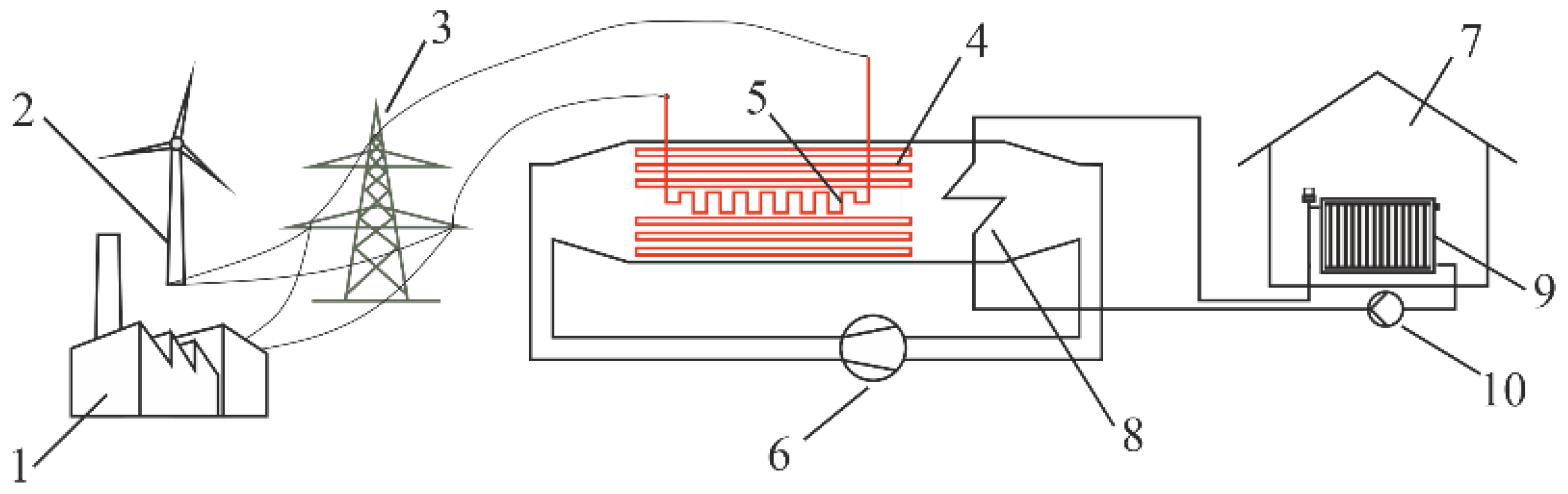
Solid-fill heat accumulators are typically used for direct space heating. The electrically heated storage unit analysed in this paper can be used as a heat source in a hydronic central heating system for a building. In this way, solid-fuel-, oil-, or gas-fired boilers can be eliminated from existing building heating systems. The electrically heated accumulators can be used to capture excess electricity from wind farms. In summer, the heat stored in the accumulator can be used to heat domestic hot water. An example of using a heat accumulator to heat a building is shown in Figure 1.

During the period of overproduction of electricity in the system, which usually occurs during the night, the heat storage unit is heated using electricity. During the night period, the demand for electricity is low. Thermal power plants operate with the minimum allowable load, as it is not worthwhile to shut them down due to the very high restart costs. In addition, the wind velocity during the night period is usually higher than during the day, resulting in increased output from wind farms. Due to the excess of electricity during the night period when electricity demand is low, the electricity supply is greater than the electricity demand. This results in an extreme reduction in the electricity price per kWh at night. One way to utilise this excess electricity is through heat accumulators with a fixed packing, which can be heated to a high temperature; e.g., up to 600 °C. When electricity prices rise due to increased demand during the daytime period, the heat accumulator is not supplied with electricity. During the day, the accumulator is discharged using the air flowing through it. The accumulator can be located in a heated room, or it can replace a conventional fossil fuel-fired boiler situated in the boiler room. The latter solution is very beneficial for historic city centres, where there are many old buildings without access to a central heating network. A favourable alternative to replacing a masonry heater (tiled stove) or other heat sources is a designed accumulator that does not emit harmful substances. By heating the accumulator using inexpensive electricity in times of low demand, the heating costs are competitive with other techniques to heat buildings. A central heating system in which an accumulator has replaced a conventional gas-fired boiler is shown in Figure 1. The accumulator, which is heated up during the night, is cooled down by flowing air that is then cooled down in a finned air–water heat exchanger. This heat exchanger works as a central heating boiler. The proposed solution is simple and inexpensive.

This paper developed a new simple numerical model of the heat storage unit. A new method for determining the correlation for the heat transfer coefficient from the packing surface to the flowing air was proposed using the least-squares method. The accuracy of the numerical accumulator models was assessed by comparing the air and packing temperatures at the accumulator outlet with those obtained using an analytical exact solution that was obtained using the superposition method. A numerical mathematical model of the accumulator based on the explicit Euler method and the Crank–Nicolson method was verified by exact solutions for a step change in air temperature at the inlet to the accumulator and a ramp change in inlet air temperature. The verification of numerical solutions is of great importance in the case of heat accumulators. If the number of finite volumes is too low, the accuracy of the numerical solutions can frequently be unsatisfactory [14]. Compared to heat conduction, the number of finite volumes along the length of the accumulator needs to be greater or several times higher to achieve satisfactory accuracy of the accumulator modelling. The computer calculation time using the developed model, especially using the Crank–Nicolson method, was very short. This made it possible to apply the developed numerical model in an automatic air temperature control system. In the predictive air temperature control, the proposed mathematical model of the heat storage unit could be used to determine the fan rotational speed so that the air temperature at its outlet was equal to the set temperature. In this way, despite the discharging of the accumulator during the day; i.e., a decrease in the packing temperature, it was possible to maintain the set temperature in the heated room by changing the airflow velocity.

2. Design of the Heat Accumulator

A laboratory test stand was built to test an electric–water heating system for a building. The air heated in the accumulator gave up heat to the water flowing in the finned heat exchanger (car radiator), which in turn was the heat source for the central heating system.

Figure 2a shows a hybrid electric–water building heating system using a dynamic discharge heat accumulator, while a photograph of the heating system test rig is shown in Figure 2b. The central element of the heating system was a ceramic dynamic discharge heat accumulator with an ordered packing that was heated by low-cost electricity. The following systems can be specified in the test rig:

• An electrical sub-system for packing heating using resistance heaters; the filling of the accumulator was composed of ceramic and steel elements;
• A water circuit comprising a plate-finned and tube heat exchanger (PFTHE), central heating radiators, a water circulation pump, and pipes through which the water flowed;
• An air-circulation sub-system consisting of the heat accumulator, a radial forced draft fan, and the PFTHE;
• A power and control unit;
• Measuring equipment with a data-acquisition system.

The hybrid electric–water heating system for a building analysed in the paper is presented in Figure 2. The Heat accumulator ➀ (Figure 2a) as a heat source in a central heating system was heated by resistance heaters during periods of low electricity demand; i.e., at night or during midday hours when electricity was inexpensive. This type of heating system is particularly cost-effective in countries where electricity is inexpensive; e.g., in countries with a high proportion of nuclear, hydroelectric, or wind power stations in the energy system.

In the heat storage unit ➀, a dynamic heat discharge was used. On the outer surface, the accumulator was well thermally insulated. Heat was extracted from the high-temperature filling by flowing air that, after heating, was cooled in the PFTHE ➁, which was composed of oval tubes with continuous fins. The capacity of the PFTHE was about 20 kW when the air velocity before entering the heat exchanger was approximately 3 m/s. The area of continuous fins in the heat exchanger was several times larger than the area of the plain tubes, so the PFTHE dimensions and its cost were small. The water temperature in the central heating system supply had to be maintained with a controller to ensure a constant temperature in the room. A centrifugal pump forced the water flow in the central heating system. The water temperature at the PFTHE outlet could be changed by varying the rotational speed of the fan ➃ or by changing the number of pump impeller revolutions. The centrifugal fan ➃ forced the air through the PFTHE.

The PFTHE ➁ was located at the outlet of the heat accumulator in the left lower part of the test stand. The fan ➃ forced air through the accumulator. A water flow meter was situated in the centre of the stand above the accumulator.

The water circuit in the hybrid heating system consisted of a PFTHE, a central heating system with plate radiators, and a water circulation pump. The PFTHE was an automotive radiator used in spark-ignition engines with a capacity of 1600 cm³. The air heated in the accumulator was used to heat the water in the PFTHE, which performed the function of a classic boiler in a central heating system. The purpose of plate radiators in the installation was to dissipate the heat absorbed by the air as it flowed through the accumulator. The panel radiators were located in an adjacent room to avoid heating the air where the test rig was located. The water temperature in the central heating radiators decreased by the same number of degrees. This ensured a stable internal temperature during the tests.

The hot water at the outlet of the lamella heat exchanger was the feed water for the central heating system. The water temperature in the central heating radiators dropped by the same amount as it heated up in the PFTHE. This ensured that the entire hybrid system operated under steady-state conditions. The water flow in the central heating system was regulated by changing the rotational speed of the circulation pump via a current frequency converter. A centrifugal fan with a drive motor of 1.5 kW forced the air through the heat accumulator. The maximum volumetric capacity of the fan was 660 m³/h and the maximum air pressure was 4.2 kPa.

The heat accumulator with dynamic discharge was the main component in the hybrid heating system. The principle of the heat accumulator operation was based on the use of clean energy such as electricity, including electricity from renewable energy sources.

The heat storage unit consisted of two basic components: the outer casing and the core (packing). The outer casing was a steel tube made of heat-resistant steel. The cylindrical shape of the casing provided advantages that are not present in traditional accumulation heaters. The air flow through the circular cross-section of the battery was more uniform compared to the rectangular cross-section of the housing.

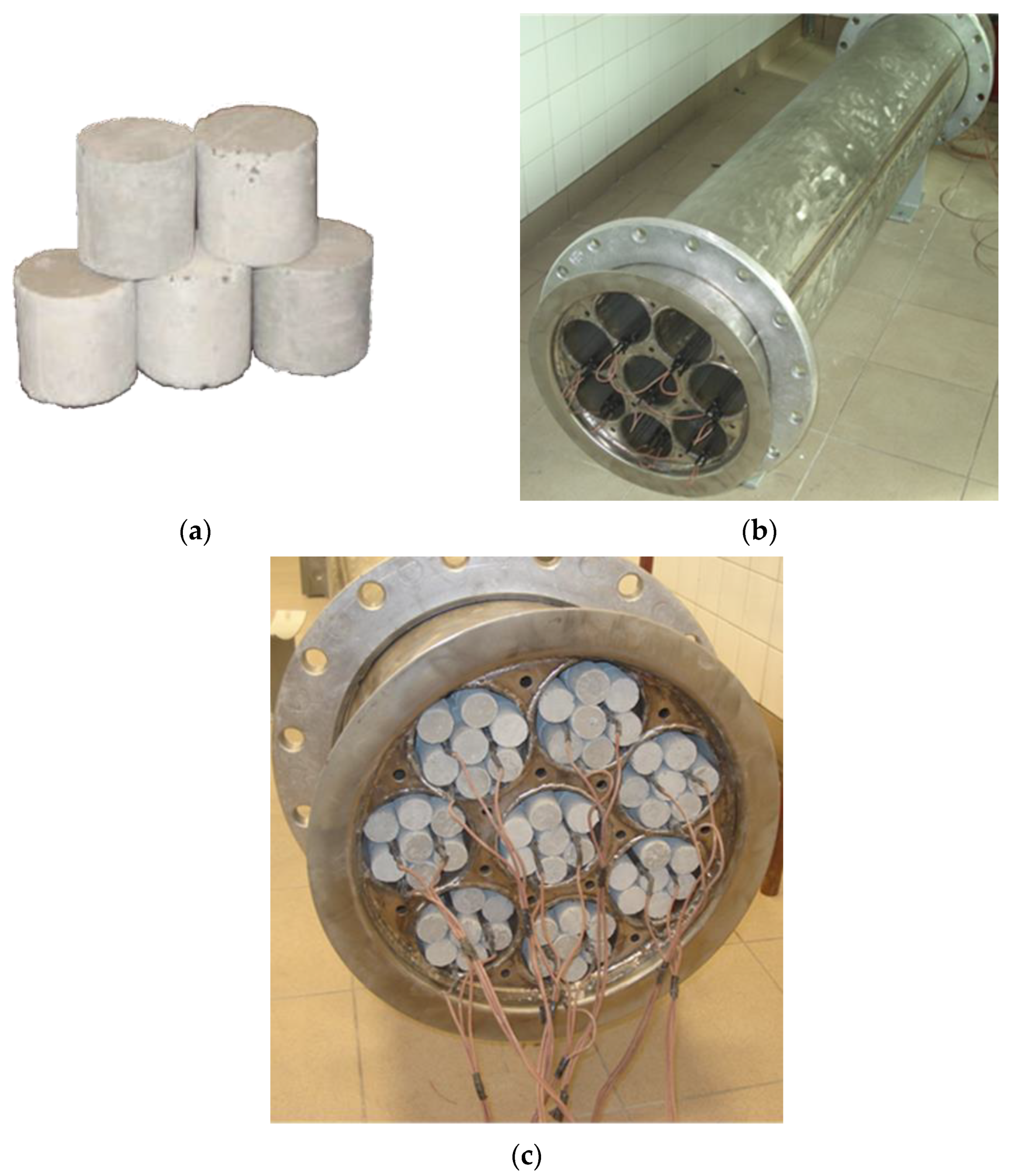
The filling of the accumulator consisted of cylindrical ceramic elements heated during the night using inexpensive electric energy. A view of the accumulator packing is illustrated in Figure 3a, and the dimensions of the outer shell and regenerator components are shown in Figure 3b.

Eight steel tubes (4) with an external diameter of 101.6 mm and a wall thickness of 3.6 mm were inside the outer casing (3) (Figure 3). Three electric heaters (2) were placed in each tube. Seven rows of cylinders (1) formed by cylinders of an equal diameter and height of 30 mm were inside each of the steel tubes along their entire lengths. The ceramic cylinders were made of heat-resistant corundum concrete. The packing of the accumulator then had an arranged structure. The air flowed longitudinally around the ceramic elements inside the steel tubes. An additional air stream flowed between the steel tubes on the shell side. Air enters the inter-tube space through 14 holes (6) that were 20 mm in diameter (Figure 3b). The front view of the accumulator illustrating the distribution of the ceramic elements in the steel tubes with visible connections for resistance heaters is presented in Figure 4c.

During the day, air flowed through the heat accumulator, which was pre-heated by the accumulator packing. Internal energy stored in the heated packing could be used directly for space heating or via an air–water heat exchanger to heat water in the central heating system.

The density and specific heat of the ceramic cylinders were high. As a result, the heat capacity of the accumulator also was high, and the heat stored in the accumulator was large, which in turn made it possible to heat a house with a large space. The thermal conductivity of cylinders was also significant. The thermal stresses in the cylindrical ceramic elements were therefore low, avoiding scratches and cracks.

3. Mathematical Model of a Heat Accumulator

A mathematical model of a heat accumulator was developed using the following assumptions:

• The change in temperature of the packing over time was described by a first-order ordinary differential equation;
• The air temperature was a function of time and the axial x-coordinate, and it did not change in the radial direction;
• The external surface of the accumulator was perfectly thermally insulated;
• The ceramic and steel parts of the filling and the accumulator shell were at the same temperature at a given cross-section and time.

The first assumption was commonly made in the literature on thermal modelling of heat accumulators [1]. The modelled heat storage unit met the requirements to consider the filling as an object with lumped thermal capacity. The filling element consisted of cylindrical elements and steel pipes. A body can be treated as an object of lumped heat capacity when the Biot number (Bi) for a given element is less than 0.1. A more detailed explanation of when a body can be treated as an object with a concentrated heat capacity can be found in the books by Kreith [32] and Taler and Duda [33]. In the case of the heat accumulator analysed in this paper, the maximum value of the Biot number (Bi_w = h_gd_c/(2k_w)) was less than 0.01, where d_c is the outer diameter of the ceramic cylinder, h_g is the heat transfer coefficient on the outer cylinder surface, and k_w is the ceramic cylinder thermal conductivity. In addition, for steel tubes with a wall thickness s_w equal to 3.6 mm located inside the accumulator, the Biot number (Bi), while taking into account that the tube was cooled on the external and internal surface, was Bi_w = h_gs_w/(2k_m), where k_m is the thermal conductivity of the alloyed steel of which the tubes were made. The maximum Biot number (Bi_w) shall not exceed 0.0005. Longitudinal heat conduction in exchanger walls is of secondary importance and is usually neglected [32]. This is due to the small temperature gradient of the air along its flow path. An additional factor that hinders heat conduction in cylindrical elements in the axial direction is the contact resistance at the interface between adjacent cylindrical elements. There were 67 ceramic cylinders arranged in a line along the length of the accumulator.

Figure 5 shows a circular heat storage unit, where D_w is the internal diameter of the accumulator and L_r is its length. The ordered accumulator packing consists of ceramic cylinders of diameter d_c and height H_c (Figure 5).

The energy conservation equation for air (gas) for a control volume of thickness Δx (Figure 5) has the following form:

$${\dot{m}}_g{c_{pg}|}_0^{T_g}{T_g|}_x+h{A}_{pack}\frac{\Delta x}{L_r}\left({T_w|}_{x+\frac{\Delta x}{2}}-{T_g|}_{x+\frac{\Delta x}{2}}\right)={\dot{m}}_g{c_{pg}|}_0^{T_g}{T_g|}_{x+\Delta x}+p_r{A}_w\Delta x{\rho }_g{c}_{pg}{\frac{\partial T_g}{\partial t}|}_{x+\frac{\Delta x}{2}}$$

(1)

where ${\dot{m}}_g$—air mass flow rate, kg/s; $A_w=\pi D_w^2/4$—cross-section area of the packing, m²; D_w—inner diameter of the accumulator casing, m; ${c_{pg}|}_0^{T_g}$—the mean specific heat of air at constant pressure in the temperature range from 0 °C to T_g, J/(kg·K); T_g—air temperature, °C; T_w—packing temperature, °C; h—heat transfer coefficient, W/(m²·K); A_pack—the surface area of ceramic and steel elements where heat exchange with air takes place, m²; p_r = V_g/V_c—porosity; V_g—air volume in the accumulator, m³; V_c—the total capacity of the accumulator, m³; Δx—the thickness of the control area, m; ρ_g—air density, kg/m³; L_r—accumulator length, m; c_pg(T_g)—specific heat of air at constant pressure at temperature T_g, J/(kg·K); and t—time, s.

Introducing the mean specific heat in the control volume over the temperature interval from ${T_g|}_x$ to ${T_g|}_{x+\Delta x}$ is defined as:

$$c_{pg}\left(T\right)=\frac{{c_{pg}|}_0^{T_g}{T_g|}_{x+\Delta x}-{c_{pg}|}_0^{T_g}{T_g|}_x}{{T_g|}_{x+\Delta x}-{T_g|}_x}$$

(2)

which gives:

$${\dot{m}}_g{c}_{pg}\left(T\right)\left({T_g|}_{x+\Delta x}-{T_g|}_x\right)\frac{1}{\Delta x}+p_r{A}_w{\rho }_g{c}_{pg}\frac{\partial T_g}{\partial t}=h{A}_{pack}\frac{1}{L_r}\left({T_w|}_{x+\frac{\Delta x}{2}}-{T_g|}_{x+\frac{\Delta x}{2}}\right)$$

(3)

where c_pg(T) is the specific heat of the air at constant pressure at temperature T.

When Δx → 0, then Equation (3) takes the form:

$${\dot{m}}_g{c}_{pg}\left(T\right)L_r\frac{\partial T_g}{\partial x}+p_r{A}_w{L}_r{\rho }_g{c}_{pg}\left(T\right)\frac{\partial T_g}{\partial t}=h{A}_{pack}\left(T_w-T_g\right)$$

(4)

By introducing a dimensionless coordinate x⁺ = x/L_r, Equation (4) can be written as:

$$\frac{1}{N_g}\frac{\partial T_g}{\partial x^{+}}+{\tau }_g\frac{\partial T_g}{\partial t}=T_w-T_g$$

(5)

The number of units N_g and the time constant τ_g are defined by the following expressions:

$$N_g=\frac{h{A}_{pack}}{{\dot{m}}_g{c}_{pg}}\hspace{1em}\hspace{1em}{\tau }_g=\frac{m_g{c}_{pg}}{h{A}_{pack}}$$

(6)

where $m_g=p_r{A}_w{L}_r{\rho }_g({\overline{T}}_g)$—mass of air in the accumulator, kg; p_r—packing porosity; ${\rho }_g({\overline{T}}_g)={\rho }_{gn}\left({\overline{T}}_g+273.15\right)/273.15$; ρ_gn—air density in standard temperature and pressure conditions, kg/m³; ${\rho }_g({\overline{T}}_g)$—air density at mean air temperature ${\overline{T}}_g$, kg/m³; and ${\dot{m}}_g$—mass flow rate of the air flowing through the accumulator, kg/s.

Next, the differential equation for the packing was derived. The conservation energy equation for the packing is:

$$h{A}_{pack}\frac{\Delta x}{L_r}\left({T_w|}_{x+\frac{\Delta x}{2}}-{T_g|}_{x+\frac{\Delta x}{2}}\right)+\left(m_m{c}_m+m_c{c}_c\right)\frac{\Delta x}{L_r}\frac{\partial T_w}{\partial t}=0$$

(7)

where T_w—packing temperature, °C; m_m—the mass of the steel structural components inside the accumulator including the mass of the accumulator casing, kg; c_m—stainless steel specific heat, J/(kg·K); m_c—the mass of the ceramic packing elements, kg; and c_c—specific heat of packing elements, J/(kg·K).

Transformation of Equation (7) to dimensionless form gives:

$${\tau }_w\frac{\partial T_w}{\partial t}=-\left(T_w-T_g\right)$$

(8)

where τ_w is given by the following relation:

$${\tau }_w=\frac{m_m{c}_m+m_c{c}_c}{h{A}_{pack}}$$

(9)

Equations (5) and (8) describe the changes in air and packing temperature as a function of time.

The boundary condition for air and the initial temperatures for air and packing have the following forms:

$${T_g|}_{x^{+}=0}=T_g^{\prime }\left(t\right)$$

(10)

$${T_g|}_{t=0}=T_0$$

(11)

$${T_w|}_{t=0}=T_0$$

(12)

where $T_g^{\prime }\left(t\right)$—the air temperature at the accumulator inlet, °C; and T₀—initial packing and air temperature, °C.

4. Modelling the Operation of a Heat Accumulator Using Exact Analytical Methods

Solutions of Equations (5) and (8) with the boundary condition (10) and initial conditions (11) and (12) can only be found for specific boundary and initial conditions when using exact analytical methods. In the general case, when the air temperature at the inlet to the accumulator is a function of time, it is not easy to find an exact analytical solution. In this paper, solutions to two problems are presented. In the first problem, the initial temperature of the packing and the air was uniformly equal to T_g,0. The air temperature at the inlet to the accumulator decreased stepwise by the value ΔT_g. In the second problem, the initial temperature of the packing and air was also equal to T₀. The air temperature at the inlet to the accumulator increased first at a constant rate v_T and then equalled the set nominal temperature T_gnom. Exact analytical solutions were used to assess the accuracy of the numerical solutions obtained using the finite-difference method.

4.1. Exact Analytical Solution for a Step Change in the Air Temperature at the Heat Accumulator Inlet

The temperature of the air flowing through the heat accumulator was a function of time and position. The operation of the heat accumulator was modelled when the air temperature at the inlet to the accumulator was stepped down (Figure 6).

The differential equations describing the air and packing temperatures as a function of time and position were derived under the following simplifying assumptions:

• The physical properties of the air and the ceramic packing were constant;
• The packing temperature was a function of time only;
• The air temperature was a function of time t and the x-coordinate, and in a given cross-section, the air temperature is uniform;
• The external surface of the accumulator was wholly insulated, and heat transfer took place only between the packing and the air flowing through the accumulator.

Changes in the air temperature inside the accumulator were described by the conservation of energy Equation (5) and the packing temperature by Equation (8).

The system of Equations (5) and (8) was solved with the following boundary condition:

$${T_g|}_{x=0}=T_{g,in}$$

(13)

The initial temperature of the air and the accumulator packing was constant and equal to T₀; i.e., the initial condition for air and wall has the following form:

$${T_g|}_{t=0}=T_{g,0}$$

(14)

$${T_w|}_{t=0}=T_{g,0}$$

(15)

By introducing temperature differences:

$${\theta }_g=T_g-T_{g,0}$$

(16)

$${\theta }_w=T_w-T_{g,0}$$

(17)

Equation (5) becomes:

$${\tau }_g\frac{\partial {\theta }_g}{\partial t}+\frac{1}{N_g}\frac{\partial {\theta }_g}{\partial x^{+}}=-\left({\theta }_g-{\theta }_w\right)$$

(18)

The conservation of energy Equation (8) for accumulator packing can be written in the form

$${\tau }_w\frac{\partial {\theta }_w}{\partial t}={\theta }_g-{\theta }_w$$

(19)

The boundary condition (13) and the initial conditions (14) and (15) can be written in the following manner (Figure 6):

$${{\theta }_g|}_{x=0}=-\Delta T_g$$

(20)

$${{\theta }_g|}_{t=0}=0$$

(21)

$${{\theta }_w|}_{t=0}=0$$

(22)

The analytical solution of the system of Equations (18) and (19) for a stepwise increase in the medium temperature by −ΔT_g and initial conditions (21) and (22) has the form [31]:

$$\frac{{\theta }_g}{\Delta T_g}=-U\left(\xi ,\eta \right)\exp \left[-\left(\xi +\eta \right)\right],\hspace{1em}t\ge t_{pr}$$

(23)

$$\frac{{\theta }_w}{\Delta T_g}=-\left[U\left(\xi ,\eta \right)-I_0\left(2\sqrt{\xi \eta }\right)\right]\exp \left[-\left(\xi +\eta \right)\right],\hspace{1em}t\ge t_{pr}$$

(24)

where:

$$\xi =\frac{x{N}_g}{L_x}\hspace{1em}\hspace{1em}\eta =\frac{t-t_{pr}}{{\tau }_w}\hspace{1em}\hspace{1em}{t}_{pr}=x^{+}{N}_g{\tau }_g$$

(25)

$$U=U\left(\xi ,\eta \right)=e^{\xi +\eta }-{{\displaystyle \sum _{n=1}^{\infty }\left(\frac{\xi }{\eta }\right)}}^{\frac{n}{2}}{I}_n\left(2\sqrt{\xi \eta }\right)$$

(26)

In Equations (23), (24) and (26), I₀(x)—modified function of order zero I_n(x)—modified function of n-th order [34], and t_pr—the time of the particle passage from the inlet (x = 0) to the point of x coordinate determined by the formula t_pr = x/w_g.

4.2. Exact Analytical Solution for Changing the Air Temperature at the Inlet to the Heat Accumulator in the Form of a Ramp

Modelling of the heat accumulator was carried out using the explicit finite-difference method and the Crank–Nicolson method to test their suitability for determining the air and filling temperature distribution with time-dependent air temperature at the inlet to the accumulator. For this reason, the heat transfer in the accumulator was modelled under the particularly challenging boundary condition of a step change in temperature. Exact analytical solutions made it possible to assess the accuracy of the heat storage unit modelling using numerical methods for different time-dependent boundary conditions, as so far, there are no methods to assess the accuracy of numerical methods. There was no guarantee that both numerical methods used in the paper would give correct results.

The time–space temperature distribution during the flow of hot medium through the accumulator was determined. The initial temperature of the air and packing was constant and was equal to T₀. At the beginning of the heating process, the air temperature increased in steps by ΔT_g (Figure 7). The air temperature then rose at a constant rate v_T for the time t_cn until the temperature of the medium reached T_nom. For time t_cn ≤ t, the air temperature was constant and equal to T_nom.

The initial air and packing temperatures were assumed to be zero to simplify considerations. This assumption did not reduce the generality of the solutions obtained because the initial temperature T_g,0 had to be added to the packing and air temperatures obtained at the zero initial temperature.

The temperature distribution in the air and the pipe wall at the boundary condition shown in Figure 7a was determined using the superposition method [35]. According to this method, the air and packing temperatures were defined as the following:

$$T_g\left(x,t\right)=T_1\left(x,t\right)+T_2\left(x,t\right), 0\le t\le t_{cn}$$

(27)

$$T_w\left(x,t\right)=T_{w1}\left(x,t\right)+T_{w2}\left(x,t\right), 0\le t\le t_{cn}$$

(28)

$$T_g\left(x,t\right)=T_1\left(x,t\right)+T_2\left(x,t\right)+T_3\left(x,t-t_{cn}\right), t_{cn}\le t$$

(29)

$$T_w\left(x,t\right)=T_{w1}\left(x,t\right)+T_{w2}\left(x,t\right)+T_{w3}\left(x,t-t_{cn}\right), t_{cn}\le t$$

(30)

The boundary conditions for solutions T₁, T₂, and T₃; i.e., the change in air temperature over the time at the accumulator inlet, are shown in Figure 7b–d, respectively.

4.2.1. Solution T₁(x, t) for Air Temperature

The following differential equation describes the air temperature variation in the accumulator:

$${\tau }_g\frac{\partial T_1}{\partial t}+\frac{1}{N_g}\frac{\partial T_1}{\partial x^{+}}=-\left(T_1-T_w\right)$$

(31)

where T₁ is the excess temperature over the ambient temperature T₀. The following differential equation describes the variation of the packing temperature over the time:

$${\tau }_w\frac{\partial T_{w1}}{\partial t}=T_1-T_{w1}$$

(32)

The time changes of the air inlet temperature are described by the boundary condition (Figure 7b):

$${T_1|}_{x=0}=\Delta T_g, 0<t$$

(33)

The initial conditions have the following form:

$$T_1=0$$

(34)

$$T_{w1}=0$$

(35)

The solution of the initial-boundary problem (31)–(33) is defined as:

$$\frac{T_1-T_{g,0}}{\Delta T_g}=U\left(\xi ,\eta \right)\exp \left[-\left(\xi +\eta \right)\right],\hspace{1em}t\ge t_{pr}$$

(36)

$$\frac{T_{w1}-T_{g,0}}{\Delta T_g}=\left[U\left(\xi ,\eta \right)-I_o\left(2\sqrt{\xi \eta }\right)\right]\exp \left[-\left(\xi +\eta \right)\right],\hspace{1em}t\ge t_{pr}$$

(37)

4.2.2. Solution T₂(x, t) for Air Temperature

The differential equations describing the changes in air temperature and packing have the following forms:

$${\tau }_g\frac{\partial T_2}{\partial t}+\frac{1}{N_g}\frac{\partial T_2}{\partial x^{+}}=-\left(T_2-T_w\right)$$

(38)

$${\tau }_w\frac{\partial T_{w2}}{\partial t}=T_2-T_{w2}$$

(39)

The air temperature T₂ at the inlet to the accumulator increases linearly with time and the initial air and packing temperatures are equal to zero. The boundary condition and initial conditions have the form:

$${T_2|}_{x=0}=f_{\mathrm{I}}(t), 0\le t\le t_{cn}$$

(40)

$${T_2|}_{t=0}=0$$

(41)

$${T_{w2}|}_{x=0}=0$$

(42)

where f_I(t) = v_T t. The symbol v_T denotes the rate of change of the air temperature at the inlet to the accumulator (Figure 7c).

The solution of the initial problem (38)–(42) has the following form:

$$T_2=v_T{\tau }_w\left\{e^{-\left(\xi +\eta \right)}\left[\left(\eta -\xi \right)U+\xi I_0\left(2\sqrt{\xi \eta }\right)+\sqrt{\xi \eta }{I}_1\left(2\sqrt{\xi \eta }\right)\right]\right\}, 0\le t\le t_{cn},$$

(43)

$$T_{w2}=T_2-v_T{\tau }_w{e}^{-\left(\xi +\eta \right)}\left[U-I_0\left(2\sqrt{\xi \eta }\right)\right], 0\le t\le t_{cn},$$

(44)

where the function U is defined as follows:

$$U=U\left(\xi ,\eta \right)=e^{\xi +\eta }-{{\displaystyle \sum _{n=1}^{\infty }\left(\frac{\xi }{\eta }\right)}}^{\frac{n}{2}}{I}_n\left(2\sqrt{\xi \eta }\right)$$

(45)

where I₀(x), I₁(x), and I_n(x) denote modified Bessel functions of the zero, first, and n-th order, respectively.

4.2.3. Solution T₃(x, t) for Air Temperature

The differential equations describing the changes in air temperature and packing have the following forms:

$${\tau }_g\frac{\partial T_3}{\partial t}+\frac{1}{N_g}\frac{\partial T_3}{\partial x^{+}}=-\left(T_3-T_w\right)$$

(46)

$${\tau }_w\frac{\partial T_{w3}}{\partial t}=T_3-T_{w3}$$

(47)

The air temperature T₃ at the inlet to the accumulator increases linearly with time and the initial air and packing temperatures are equal to zero. The boundary condition and initial conditions take the form:

$${T_3|}_{x=0}=f_{\mathrm{II}}(t-t_{cn})=-{\nu }_T(t-t_{cn}), t\ge t_{cn}$$

(48)

$${T_3|}_{t=0}=0$$

(49)

$${T_{w3}|}_{t=0}=0$$

(50)

where f_II(t) = v_T(t − t_cn), t_cn ≤ t. The symbol v_T is the rate of change of the air temperature at the inlet to the accumulator (Figure 7d).

$$T_3=-v_T{\tau }_w\left\{e^{-\left(\xi +{\eta }_1\right)}\left[\left({\eta }_1-\xi \right)U+\xi I_0\left(2\sqrt{\xi {\eta }_1}\right)+\sqrt{\xi {\eta }_1}{I}_1\left(2\sqrt{\xi {\eta }_1}\right)\right]\right\}, t\ge t_{cn}$$

(51)

$$T_{w3}=T_3+v_T{\tau }_w{e}^{-\left(\xi +{\eta }_1\right)}\left[U-I_0\left(2\sqrt{\xi {\eta }_1}\right)\right], t\ge t_{cn}$$

(52)

where $\xi =\frac{x{N}_g}{L_x}$, $\eta =\frac{t-t_{pr}}{{\tau }_w}$, ${\eta }_1=\frac{t-t_{cn}-t_{pr}}{{\tau }_w}$, and $t_{pr}=x^{+}{N}_g{\tau }_g$.

The number of heat transfer units N_g, the time constant τ_g, and the wall time constant τ_w are defined by Equations (6) and (9), respectively.

5. Numerical Modelling of a Heat Accumulator

The differential equations describing the air and packing temperature changes were solved using the finite-difference method. Two finite difference schemes were used: the explicit Euler method and the Crank–Nicolson method.

The accuracy of the explicit Euler method is of the first order [36], and that of the Crank–Nicolson method [36] is the second order; i.e., the latter method is more accurate with the same number of nodes in the difference mesh. The advantage of these methods was that they could consider that the thermophysical properties of the packing and air were temperature dependent. The air temperature at the inlet to the accumulator could change over time. With the numerical methods, the accumulator air and packing temperature distribution could be determined using any temporal variation of the air temperature at its inlet. Unlike the exact analytical method, the finite difference procedure did not require the boundary condition to be a step or linear change in the air temperature.

Cooling of the accumulator filling, during which heat was extracted by the flowing air and then transferred to the finned air–water heat exchanger, was modelled using two methods: the explicit Euler method and the implicit Crank–Nicolson method. To assess the accuracy of these methods, an exact analytical solution was also found for selected temporal variations in the air temperature at the accumulator inlet. The mutual comparison of the two different numerical methods and their comparison with the exact analytical solution was necessary because, as shown in [14], the accuracy of the solutions obtained by the finite-difference (finite volume) method depends very strongly on the number of divisions of the accumulator length into calculation cells. The air temperature over the length of one cell was approximated using the arithmetic mean of the inlet and outlet temperatures for the cell. However, it turned out that the temperature distribution inside a given cell was exponential, and at low air velocities, the air temperature dropped quickly over the short length from the air inlet to the cell. In this case, the arithmetic mean did not give the true average temperature over the length of a single cell. Computational tests of air heating in an accumulator [14] have shown that when the length of the accumulator was divided into 10 control volumes, inaccurate—one might say absurd—results were obtained. For example, at an accumulator filling temperature of 300 °C, the air temperature at the heat accumulator outlet reached 500 °C, which was obviously not possible. For this reason, the assessment of the accuracy of the two numerical methods used was given more attention.

5.1. Modelling a Heat Accumulator Using an Explicit Finite-Difference Method

The system of Equations (5) and (8) with boundary condition (10) and initial conditions (11) and (12) was solved using the explicit finite-difference method. An accumulator of length L_r was divided into N finite volumes of length Δx (Figure 8). By introducing a dimensionless coordinate, the dimensionless length of the finite volume is given by the formula:

$$\Delta x^{+}=\frac{1}{N},$$

(53)

The derivative of the air temperature T_g after the x-coordinate in Equation (5) was approximated by the forward difference quotient at the old time step n, and the derivative after time by the forward difference quotient for node i + 1, which was located at the outlet of the control region contained between nodes i and i + 1. The remaining terms in Equation (5) were calculated at the old time step t_n = nΔt, n = 0, 1, …. The approximate form of Equation (5); i.e., the difference equation, is as follows:

$${\tau }_{g,i}^n\frac{T_{g,i+1}^{n+1}-T_{g,i+1}^n}{\Delta t}+\frac{1}{N_{g,i}^n}\frac{T_{g,i+1}^n-T_{g,i}^n}{\Delta x^{+}}=T_{w,i}^n-\frac{T_{g,i}^n+T_{g,i+1}^n}{2}$$

(54)

The finite-difference grid is defined as follows:

$$x_i=(i-1)\Delta x,\hspace{1em}\Delta x=L_r/N,\hspace{1em}{x}_i^{+}=x_i/L_r\hspace{1em}i=1,\dots ,\left(N+1\right)\hspace{1em}{t}_n=n\Delta t,\hspace{1em}n=0,1,\dots$$

(55)

The differential Equation (8) was approximated in a similar way:

$${\tau }_{w,i}^n\frac{T_{w,i}^{n+1}-T_{w,i}^n}{\Delta t}=-\left(T_{w,i}^n-\frac{T_{g,i}^n+T_{g,i+1}^n}{2}\right)\hspace{1em}i=1,\dots ,\left(N+1\right)\hspace{1em}n=0,1,\dots$$

(56)

Solving Equation (54) for $T_{g,i+1}^{n+1}$ gives:

$$T_{g,i+1}^{n+1}=T_{g,i+1}^n+\frac{\Delta t}{{\tau }_{g,i}^n}\left[\left(T_{w,i}^n-\frac{T_{g,i}^n+T_{g,i+1}^n}{2}\right)-\frac{1}{N_{g,i}^n}\frac{T_{g,i+1}^n-T_{g,i}^n}{\Delta x^{+}}\right],i=1,\dots ,N\hspace{1em}n=0,\dots$$

(57)

The wall temperature $T_{w,i}^{n+1}$ was determined using Equation (56):

$$T_{w,i}^{n+1}=T_{w,i}^n-\frac{\Delta t}{{\tau }_{w,i}^n}\left(T_{w,i}^n-\frac{T_{g,i}^n+T_{g,i+1}^n}{2}\right),i=1,\dots ,N\hspace{1em}n=0,1,\dots$$

(58)

The system of difference Equations (57) and (58) was solved with the boundary condition (10), which takes the form:

$$T_{g,1}={\left(T_g^{\prime }\right)}^n$$

(59)

The initial conditions for gas and packing are as follows:

$$T_{g,i}^0=T_0\hspace{1em}\hspace{1em}i=1,\dots ,N+1$$

(60)

$$T_{w,i}^0=T_0\hspace{1em}\hspace{1em}i=1,\dots ,N$$

(61)

From Equations (57) and (58), the air and packing temperatures were determined as a function of location and time while taking into account the boundary condition (59) and the initial conditions (60) and (61). The time step Δt should satisfy the Courant–Friedrichs–Lewy condition [36]:

$$\frac{\Delta t}{N_g{\tau }_g\Delta x^{+}}\le 1$$

(62)

Due to the small value of the product ρ_gc_pg, the heat accumulated in the air is minimal. Therefore, air temperature changes over time occur very quickly. Disregarding the heat accumulation in the air; i.e., assuming τ_g = 0, a simplified form of the differential Equation (5) is as follows:

$$\frac{1}{N_g}\frac{\partial T_g}{\partial x^{+}}=T_w-T_g$$

(63)

Replacing the derivatives in Equation (63) with the difference quotient yields:

$$\frac{1}{N_{g,i}^n}\frac{T_{g,i+1}^{n+1}-T_{g,i}^{n+1}}{\Delta x^{+}}=T_{w,i}^{n+1}-\frac{T_{g,i}^{n+1}+T_{g,i+1}^{n+1}}{2}$$

(64)

The solution of Equation (64) for $T_{g,i+1}^{n+1}$ has the following form:

$$T_{g,i+1}^{n+1}=\frac{1}{1+\frac{\Delta x^{+}}{2N_{g,i}^n}}\left[\frac{\Delta x^{+}}{N_{g,i}^n}{T}_{w,i}^{n+1}+T_{g,i}^{n+1}\left(1-\frac{\Delta x^{+}}{2N_{g,i}^n}\right)\right],\hspace{1em}i=1,\dots ,N\hspace{1em}n=0,1,\dots$$

(65)

The packing temperature is calculated using the relationship (58) with boundary condition (59) and initial conditions (60) and (61).

Assuming zero air heat capacity, the computer simulation time is greatly reduced, as there is no Courant–Friedrichs–Lewy stability condition on time-step length Δt (62). At low air velocities, the air temperature rise per control volume is large, and the approximation of the average temperature by the arithmetic mean of the inlet and outlet temperatures, as in Equation (54) or Equation (64), is insufficiently accurate [14]. The accumulator length must be divided into a large number of control volumes; e.g., assume N = 50 or more to ensure high calculation accuracy at low air velocities [14].

5.2. Modelling a Heat Accumulator Using the Crank–Nicolson Method

In the Crank–Nicolson method [36], the derivative after time in the differential equations for air and packing was approximated by the forward difference quotient. The arithmetic mean of the values approximated the remainder of the equation at the beginning and end of a given time step. Equation (5) can be written in the following form:

$${\tau }_g\frac{\partial T_g}{\partial t}=-\frac{1}{N_g}\frac{\partial T_g}{\partial x^{+}}+\left(T_w-T_g\right)$$

(66)

Equation (66) was approximated by the following difference scheme using the Crank–Nicolson method:

$$\begin{array}{l}\frac{1}{2}\left({\tau }_{g,i}^n+{\tau }_{g,i}^{n+1}\right)\frac{T_{g,i+1}^{n+1}-T_{g,i+1}^n}{\Delta t}=\frac{1}{2}\{\left[-\frac{1}{N_{g,i}^n}\frac{T_{g,i+1}^n-T_{g,i}^n}{\Delta x^{+}}+\left(T_{w,i}^n-\frac{T_{g,i}^n+T_{g,i+1}^n}{2}\right)\right]+\\ +\left[-\frac{1}{N_{g,i}^{n+1}}\frac{T_{g,i+1}^{n+1}-T_{g,i}^{n+1}}{\Delta x^{+}}+\left(T_{w,i}^{n+1}-\frac{T_{g,i}^{n+1}+T_{g,i+1}^{n+1}}{2}\right)\right]\}\hspace{1em}i=1,\dots ,N,\hspace{1em}n=0,1,\dots \end{array}$$

(67)

Equation (8) for the accumulator packing was transformed in a similar manner:

$$\begin{array}{l}\frac{1}{2}\left({\tau }_{w,i}^n+{\tau }_{w,i}^{n+1}\right)\frac{T_{w,i}^{n+1}-T_{w,i}^n}{\Delta t}=-\frac{1}{2}\left[\left(T_{w,i}^n-\frac{T_{g,i}^n+T_{g,i+1}^n}{2}\right)+\left(T_{w,i}^{n+1}-\frac{T_{g,i}^{n+1}+T_{g,i+1}^{n+1}}{2}\right)\right]\\ \\ \hspace{1em}\hspace{1em}\hspace{1em}\hspace{1em}\hspace{1em}\hspace{1em}\hspace{1em}\hspace{1em}\hspace{1em}\hspace{1em}\hspace{1em}\hspace{1em}\hspace{1em}\hspace{1em}\hspace{1em}\hspace{1em}\hspace{1em}\hspace{1em}\hspace{1em}i=1,\dots ,N,\hspace{1em}n=0,1,\dots \end{array}$$

(68)

The system of Equations (67) and (68) was solved for $T_{g,i+1}^{n+1}$ and $T_{w,i}^{n+1}$. To solve the system of Equations (67) and (68), the Thomas method [37], also known as the tri-diagonal matrix algorithm, was used. The Thomas algorithm is a particular case of the Gauss elimination method that does not require inversion of the coefficient matrix. The unknowns in the system of equations were determined using simple analytical formulas. Therefore, the time needed for numerical calculation was very short. The set of Equations (67) and (68) can also be solved with the iterative method of Gauss–Seidel. The temperatures $T_{g,i+1}^n$ and $T_{w,i}^n$ were taken as initial values in the iterative process. Due to the insignificant differences between $T_{g,i+1}^{n+1}$ and $T_{g,i+1}^n$ and between $T_{w,i}^{n+1}$ and $T_{w,i}^n$ the number of iterative steps required to obtain the solution was small.

5.3. Computational Tests

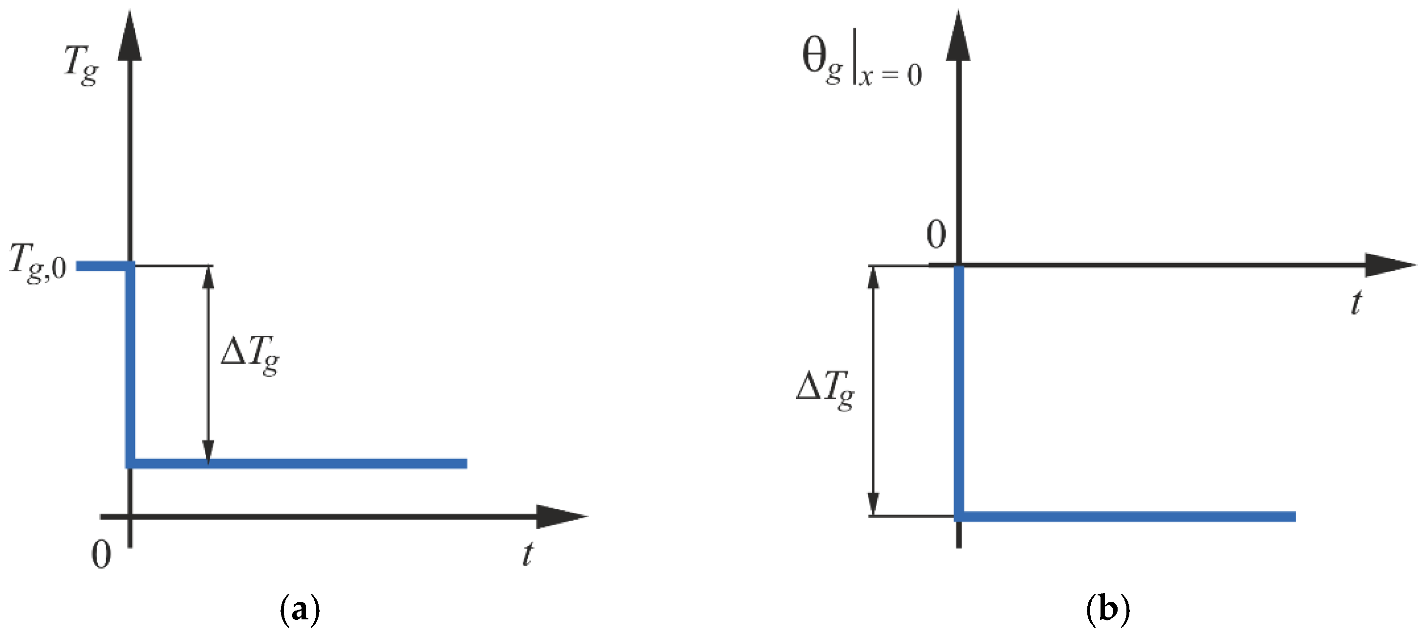
Two cases of a change in inlet air temperature were considered. In the first case, the air temperature decreased stepwise from an initial temperature T₀ = 600 °C to an ambient temperature of 20 °C (Figure 9). In the second case, the initial air and packing temperature increased stepwise from initial temperature T₀ = 0 °C to 100 °C, then rose at a constant rate of 0.25 K/s and then remained constant after reaching 600 °C (Figure 10).

The results shown in Figure 9 and Figure 10 were obtained for the following data calculated for the accumulator discussed in Section 2: N_g = 1.275, τ_w = 1013.627 s, τ_g = 0.3577 s, h_g = 11.55 W/(m²·K), N = 20, and Δt = 0.005. Figure 10 shows the results of the calculations obtained for the same data except for the number of nodes, which was (N + 1) = 65.

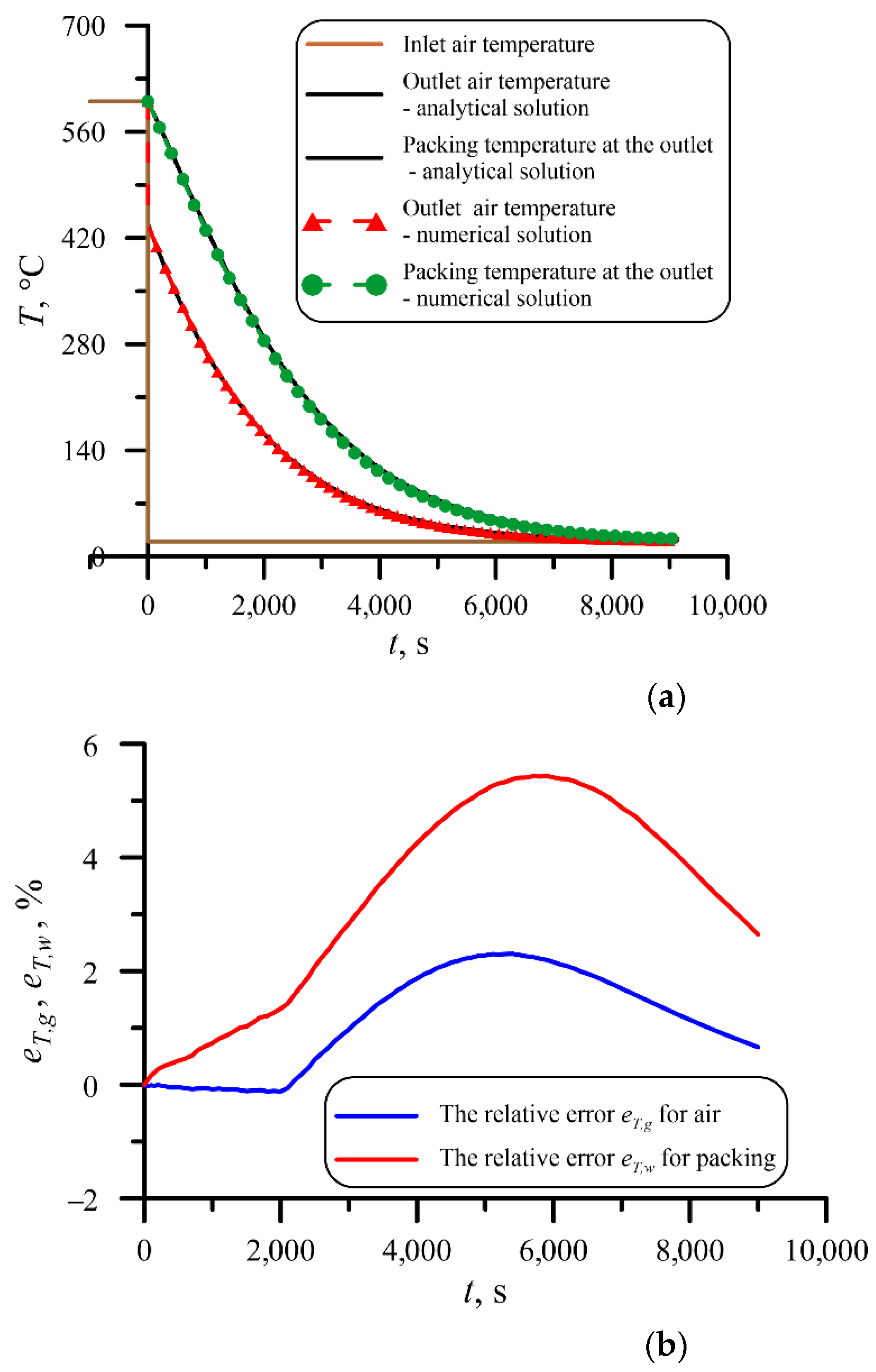
The analysis of the results shown in Figure 9 demonstrated that even with a small number of nodes along the length of the regenerator, the agreement between the air and packing temperatures at the outlet of the regenerator calculated using the exact analytical method and the explicit finite-difference method was very good.

The relative values of the difference between the air temperature determined by the exact analytical formula and the finite-difference method were calculated using the following formula:

$$e_{T,g}=100\frac{{T_g^{exact}|}_{x=L_r}-{T_g^{num}|}_{x=L_r}}{{T_g^{exact}|}_{x=L_r}},\hspace{1em}\%$$

(69)

The relative difference was calculated analogously for the packing temperatures:

$$e_{T,w}=100\frac{{T_w^{exact}|}_{x=L_r}-{T_w^{num}|}_{x=L_r}}{{T_w^{exact}|}_{x=L_r}},\hspace{1em}\%$$

(70)

where $T_g^{exact}$ and $T_w^{exact}$—air and packing temperatures calculated using an exact analytical method, respectively; and $T_g^{num}$ and $T_w^{num}$—air and packing temperatures calculated using a numerical method, respectively.

The maximum value of e_T,g = 2.3% occurred at time t = 5400 s and the maximum value of e_T,w = 5.43% at time t = 5700 s (Figure 9b).

The relative differences between the exact analytical solution and the numerical solution were smaller for the second case analysed due to the larger number of nodes equal to (N + 1) = 65 and the use of the Crank–Nicolson method to solve the system of equations, which had a second order of accuracy; i.e., it was more accurate than the explicit finite-difference method, the order of accuracy of which was one.

The absolute maximum relative difference values were e_T,g = 0.425% and e_T,w = 1.20% for the explicit finite-difference method and e_T,g = 0.424% and e_T,w = 1.20% for the Crank–Nicolson method (Figure 10b).

From a comparison of the results shown in Figure 9b and Figure 10b, it can be seen that the accuracy of calculations using the explicit finite-difference method increased as the number N of finite volumes increased. When increasing N from 20 to 64, the relative error e_T,g for air decreased by 5.4 times and for packing e_T,w by 4.5 times. When dividing the pipe into N = 64 finite volumes (Figure 10b), the Crank–Nicolson method gave similar results to the explicit finite-difference method due to a large number of finite volumes. The computational tests carried out demonstrated that both the explicit finite-difference method and the Crank–Nicolson method could be used to simulate the operation of the accumulator under analysis. The accuracy of such a simulation was significantly affected by the number of finite volumes, especially at low air velocity. In order to achieve sufficient calculation accuracy, it is recommended that N ≥ 50.

6. Experimental Verification of the Developed Numerical Model of Accumulator Discharge

The packing of the heat accumulator under test consisted of cylindrical ceramic elements and pipes, as well as other steel elements. For modelling, the following thermophysical properties and dimensions of the accumulator construction elements were assumed: Prandtl number for air, Pr_g = 0.7; air thermal conductivity, k_g = 0.236 W/(m·K); kinematic viscosity of the air, ν_g = 16.35·10⁻⁶ m²/s; air density at 50 °C, ρ_g = 1.09 kg/m³; air specific heat at constant pressure, c_p,g = 1000.0 J/(kg·K); air velocity before the packing, w_g = 2.0 m/s; stainless steel thermal conductivity, k_m = 14.7 W/(m·K); stainless steel density, ρ_m = 7800 kg/m³; steel specific heat, c_m = 519 J/(kg·K); total mass of steel elements, m_m = 252.8 kg; heat accumulator casing cross-sectional area, A_r = 2.17 m²; length of heat accumulator, L_r = 2 m; thermal conductivity of ceramic cylinder, k_w = 6.4 W/(m·K); density of ceramic cylinder, ρ_w = 2700 kg/m³; specific heat of ceramic cylinder, c_w = 519 J/(kg·K); total mass of ceramic packing, m_w = 252.8 kg; and ceramic packing outer surface area, A_w = 22.57 m².

Air temperature measurements were carried out using K-type sheathed thermocouple sensors with a grounded junction. All thermocouples were pre-calibrated using a Pt100 platinum resistance sensor. The thermocouples were selected so that when measuring air temperatures below 100 °C, their readings would be the same with an accuracy of ±0.1 K. Uncertainty of temperature measurement in the air temperature range of −20 °C to +100 °C was assumed as for a resistance temperature sensor Pt100; i.e., ±0.35 K

Air velocity was measured using a digital vane anemometer with a maximum resolution of 0.01 m/s. The uncertainty of the sensor was ±0.5% of the upper limit of the measuring range or ±1.5% of the measured value.

Due to the lack of dependence in calculating the heat transfer coefficient between the air and the elements of the heat accumulator with such a complex packing structure, a procedure for determining the mean heat transfer coefficient was developed.

The accumulator we built and tested was characterised by a complex flow and heat system inside the packing. Part of the air stream flowed inside the tubes in which the cylindrical filling elements were placed, and the other part flowed outside between the steel tubes. The air-side heat transfer coefficient h_a was approximated using the following formula:

$$h_g=a+b{\overline{w}}_g^c$$

(71)

where a, b, and c are constants to be determined.

The heat transfer coefficient h_g in Formula (71) is expressed in W/(m²·K) and the mean air velocity through the accumulator ${\overline{w}}_g^c$ in m/s.

The mean velocity of air flow through the whole cross-section of the accumulator is calculated as:

$${\overline{w}}_g=\frac{{\dot{m}}_g}{{\overline{\rho }}_g{A}_g}$$

(72)

The free area A_g of the cross-section of the accumulator through which air flows is given by:

$$A_g=\epsilon \pi R_w^2$$

(73)

where ε is the porosity of the entire accumulator packing and R_w is the internal diameter of the accumulator casing.

All constants in Equation (71) were selected so that the measured and calculated air temperature at the outlet from the accumulator agreed as well as possible. Constants a, b, and c were determined from the condition:

$$S=S\left(a,b,c\right)={\displaystyle \sum _{i=1}^{n_m}{\left[T_{g,out}^{meas}\left(t_i\right)-T_{g,out}^{calc}\left(t_i\right)\right]}^2}\to \min$$

(74)

The air temperature $T_{g,out}^{calc}$ at the outlet from the accumulator for selected time points t_i, i = 1,…, n_m was calculated using the developed mathematical model.

The constants a, b, and c in correlation (71) were determined from condition (74). The constants a*, b*, and c* at which the function S reached its minimum were determined using the Nelder–Mead method [38]. A library program for optimisation using the Nelder–Mead method can also be found in the IMSL library [39]. Calculations were performed with the use of MATLAB [40] using the FMINSEARCH program. In this paper, the number of measurement points was 1956. The air temperature at the battery outlet was measured with a step equal to 5 s. The total air temperature measurement time was 9775 s.

Calculations of the heat accumulator under test were carried out for the following input data:

• The porosity of the accumulator packing, ε = 0.4025;
• The initial temperature of the packing and the air inside the accumulator, T₀ = 199 °C;
• Heat delivered to the accumulator packing during the charging period (heat accumulated in the packing), ΔQ_tot = 13.21 kWh.

The time changes in air velocity (w_g,inlet) and temperature at the accumulator inlet (T_g,inlet) are shown in Figure 11.

The following values of parameters appearing in Equation (71) were estimated using FMINSEARCH [39]:

$$a=1.2192,\hspace{1em}b=8.42\cdot {10}^{-5},\hspace{1em}c=13.1104$$

(75)

The time changes in the heat transfer coefficient calculated using Formula (71) and the coefficients determined using Equation (74) are shown in Figure 12.

When analyzing the results shown in Figure 12, it can be seen that the average heat penetration coefficient on all air-flown fill elements was low. This was due to the low air flow velocity inside the accumulator, as the free cross-section through which the air flowed was large.

When analyzing the results presented in Figure 13, it can be seen that at the beginning of accumulator cooling, the differences between the measured and calculated air temperature at the accumulator outlet were more significant. The maximum value of the relative difference e_T between the measured ${\left(T_g^{″}\right)}^{meas}$ and the calculated ${\left(T_g^{″}\right)}^{calc}$ of the accumulator outlet air temperature, which was calculated using the relationship $e_T=\left[{\left(T_g^{″}\right)}^{meas}-{\left(T_g^{″}\right)}^{calc}\right]/{\left(T_g^{″}\right)}^{meas}\cdot 100\%$, did not exceed 25%. For times greater than about 700 s, the relative difference e_T between the calculated and measured values of air temperature decreased to values in the order of a few percent. This was mainly due to the approximate heat transfer model in the ceramic cylinders and steel filling elements. The mathematical model of the accumulator assumed that these elements were modelled as objects with concentrated heat capacity. This meant that the temperature difference inside the ceramic cylinders and the walls of the steel tubes was not taken into account. In reality, the temperature of the elements changed with time and inside the elements as well.

7. Conclusions

Based on the calculations and measurements, the following conclusions were reached:

The investigated heat accumulator was heated at night during the period of low electricity demand when the cost of 1 kWh is low. The packing of the accumulator was heated to a temperature of about 600 °C so that the mass of the accumulator could be smaller at a given heat demand.

The developed mathematical models of the accumulator—an analytical model, a numerical model based on the explicit finite-difference method, and the implicit Crank–Nicolson method—gave similar results.

The comparison between the calculated and measured air temperatures at the accumulator outlet was satisfactory except for the initial air heating period, when the differences between the numerical solution and the measured results were more significant.

The differences in the calculated and measured values of the air temperatures at the accumulator outlet in the initial phase of the cooling of the accumulator packing were partly due to the assumption that the temperature of the filling elements was constant in the entire volume and changed only in time (model with lumped heat capacity). However, at the beginning of the cooling of the filling elements, the temperature difference inside ceramic cylinders or steel tubes could be significant. The second reason for the differences between the calculated and measured temperatures at the air outlet from the accumulator was the complex structure of the accumulator filling, which, for example, made it difficult to determine the velocity distribution in the cross-section of the packing, as well as to find appropriate correlations for calculating the heat transfer coefficient. Due to the small length of the accumulator, the heat transfer between the packing elements and the flowing air was strongly influenced by the inlet section with a developing flow, where the heat transfer coefficient was much higher than for the developed air flow.

The developed numerical model of the accumulator can be used to calculate the appropriate sizing so that it can be used to heat a building during a period of high electricity prices. The model can also be used to calculate the changes in the air temperature at the outlet of the accumulator during the entire period of its discharge (heating of a building). The elaborated dynamic mathematical model of the accumulator can also be used in an automatic temperature control system for a heated room (building) based on the mathematical model. The designed heat accumulator can replace a conventional fossil-fuel-fired boiler in a boiler room or operate as an independent unit in a heated room. In both cases, the mathematical model of the accumulator can be used in the system for automatic air temperature control in the heated space.