
Constant Power Factor Model of DFIG-Based Wind Turbine for Steady State Load Flow Studies


Abstract
:1. Introduction
- (i)
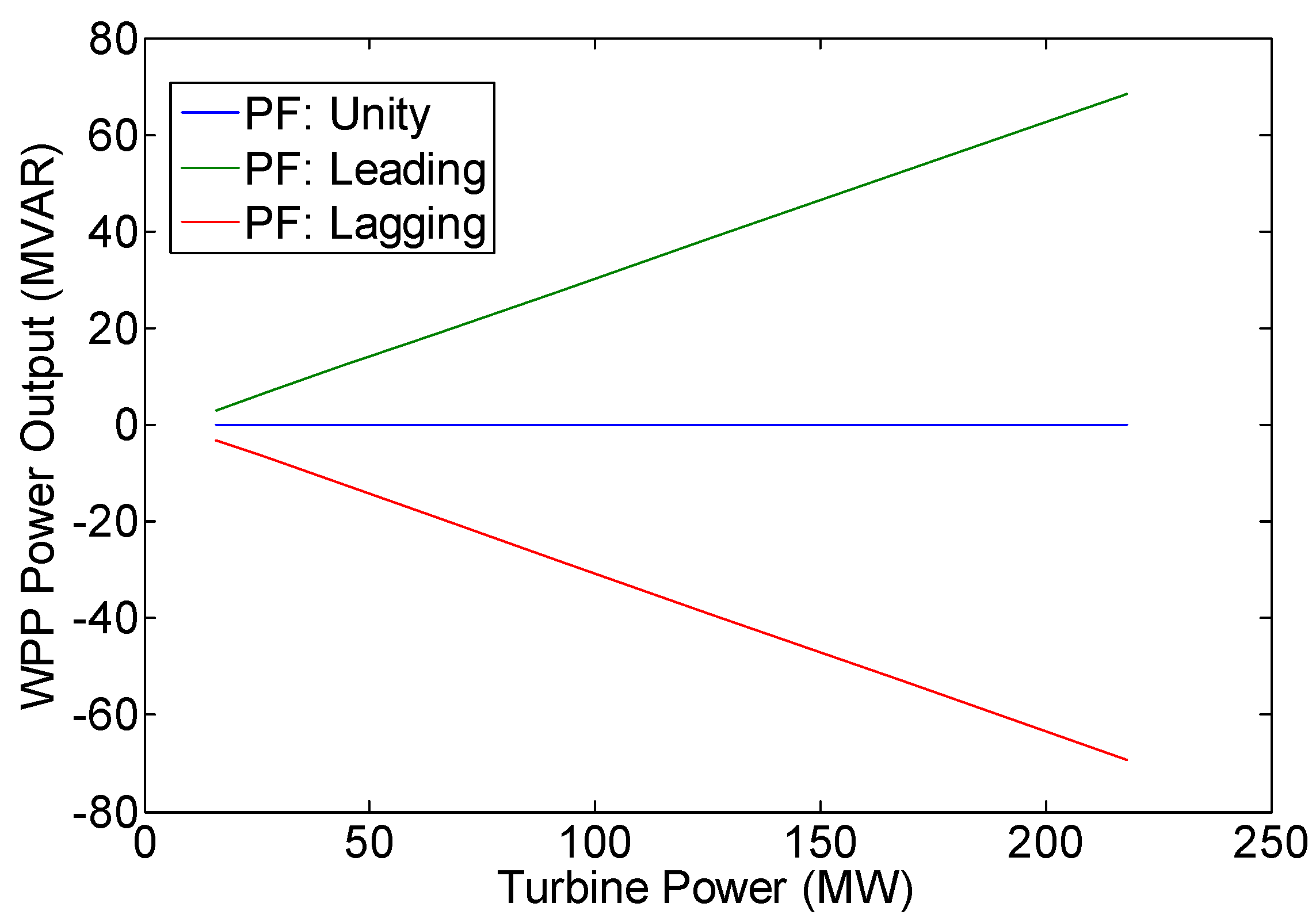
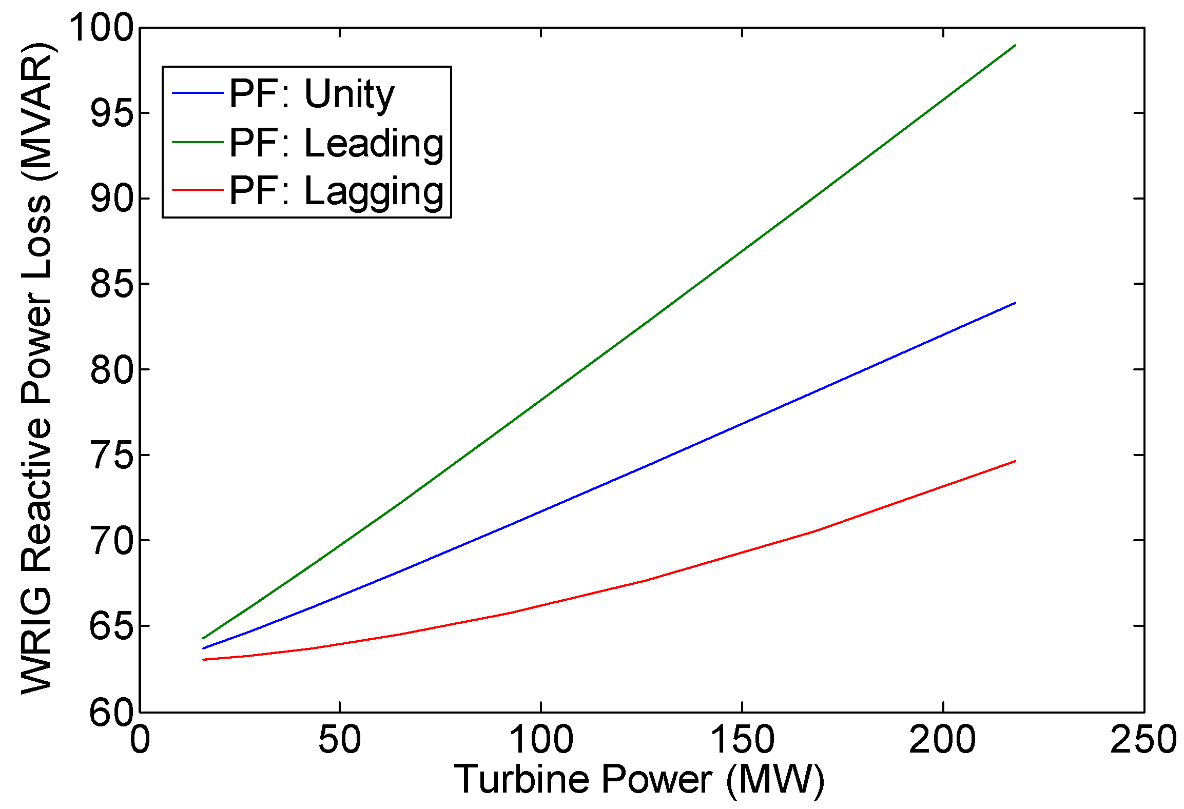
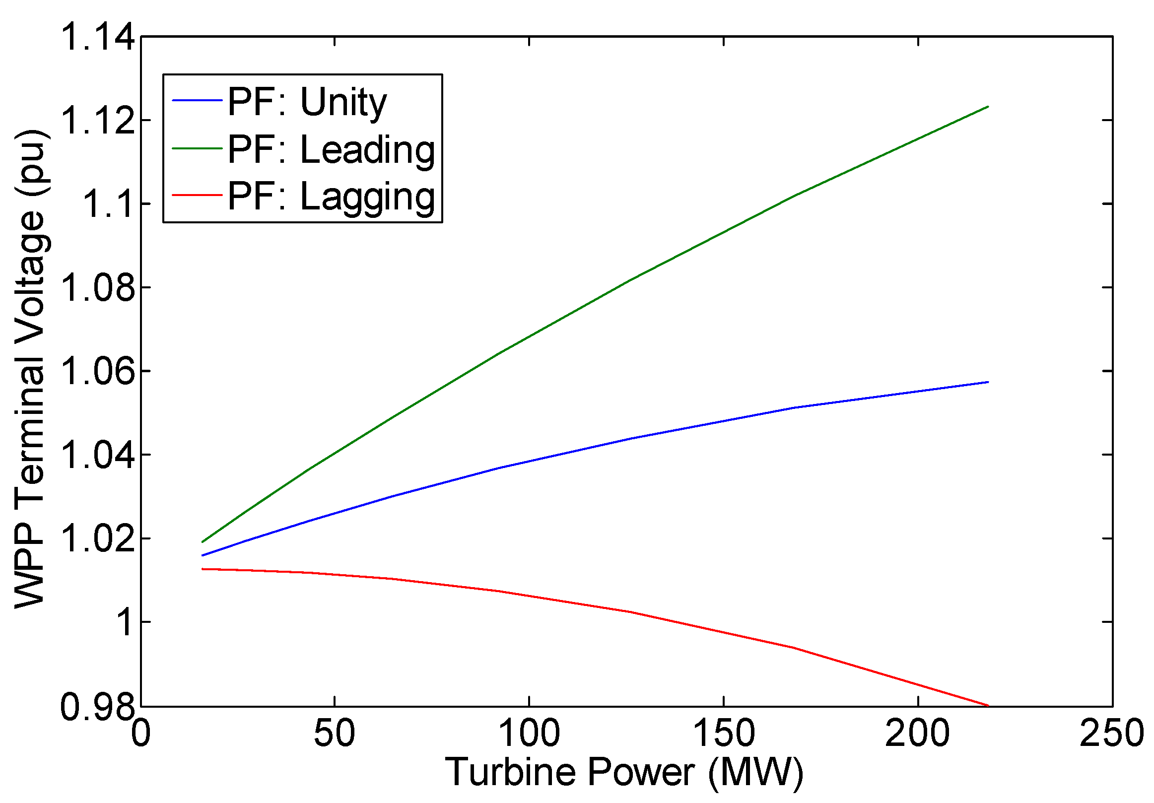
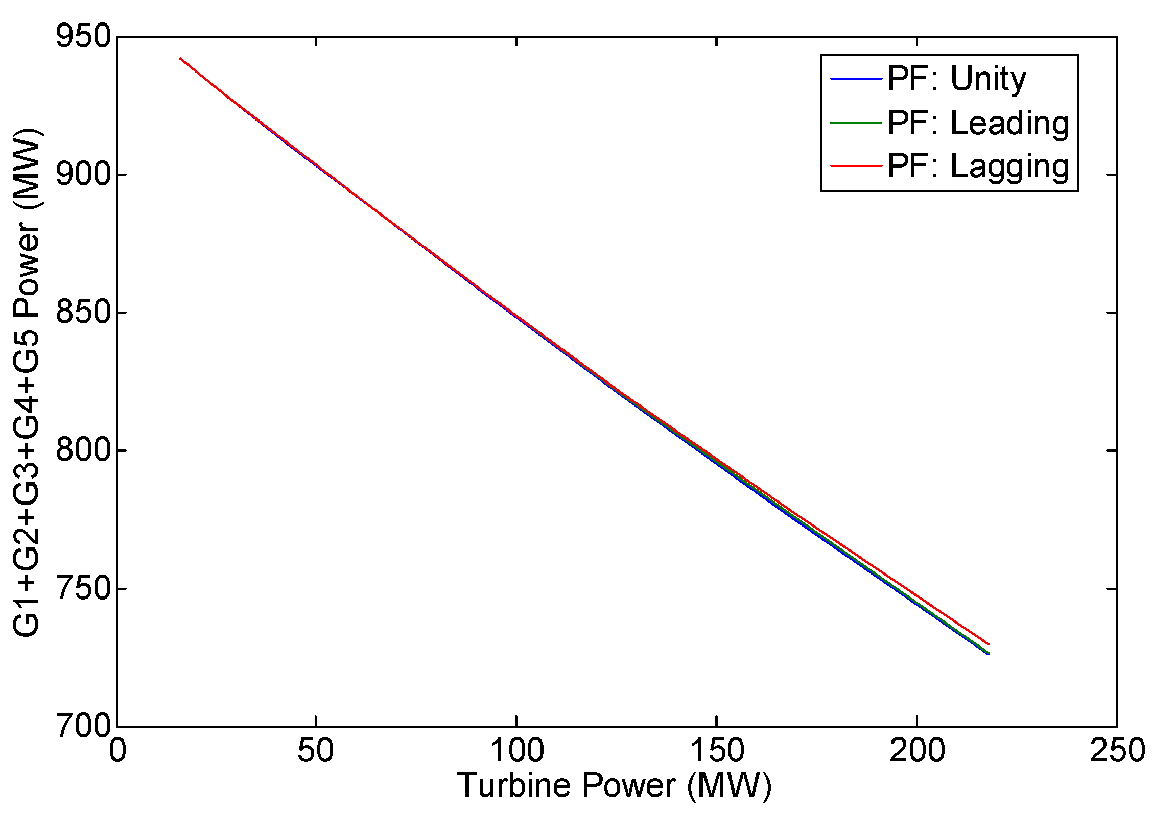
- In contrast to the methods discussed in [14,15,16,17,18,19,20] where the DFIG power factor was assumed to be constant at unity, he proposed model allows the DFIG power factor to be controlled. In addition, it can be applied not only to the unity power factor but also to lagging and leading power factor operation modes. This contribution is particularly important since DFIG-based WPP in power factor control operation mode is also often adopted in practice.
- (ii)
- Another important feature of the present paper is that representation of the DFIG in both sub-synchronous and super-synchronous conditions can be carried out by using a single mathematical model. It is to be noted that in the previously published methods [15,16,17,18], two models have to be used to represent the conditions.
2. Wind Turbine Power
| Pm | : | turbine mechanical power (Watt) |
| ρ | : | air density (kg/m3) |
| R | : | turbine blade length (m) |
| Vw | : | wind speed (m/s) |
| Cp | : | turbine performance coefficient |
| ag | : | turbine gear ratio |
| ωs | : | synchronous speed (rad/s) |
| s | : | induction generator slip |
| p | : | number of pole pairs of induction generator |
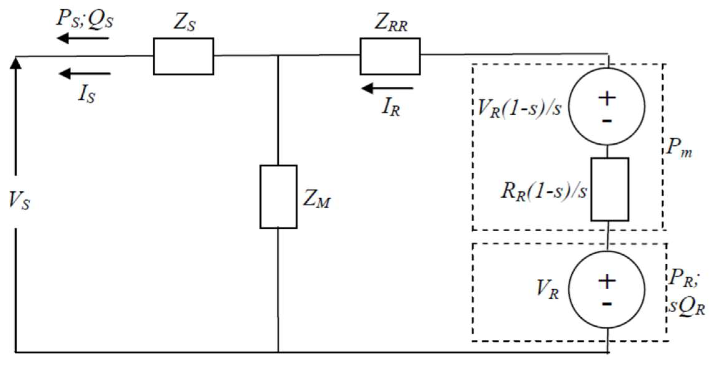
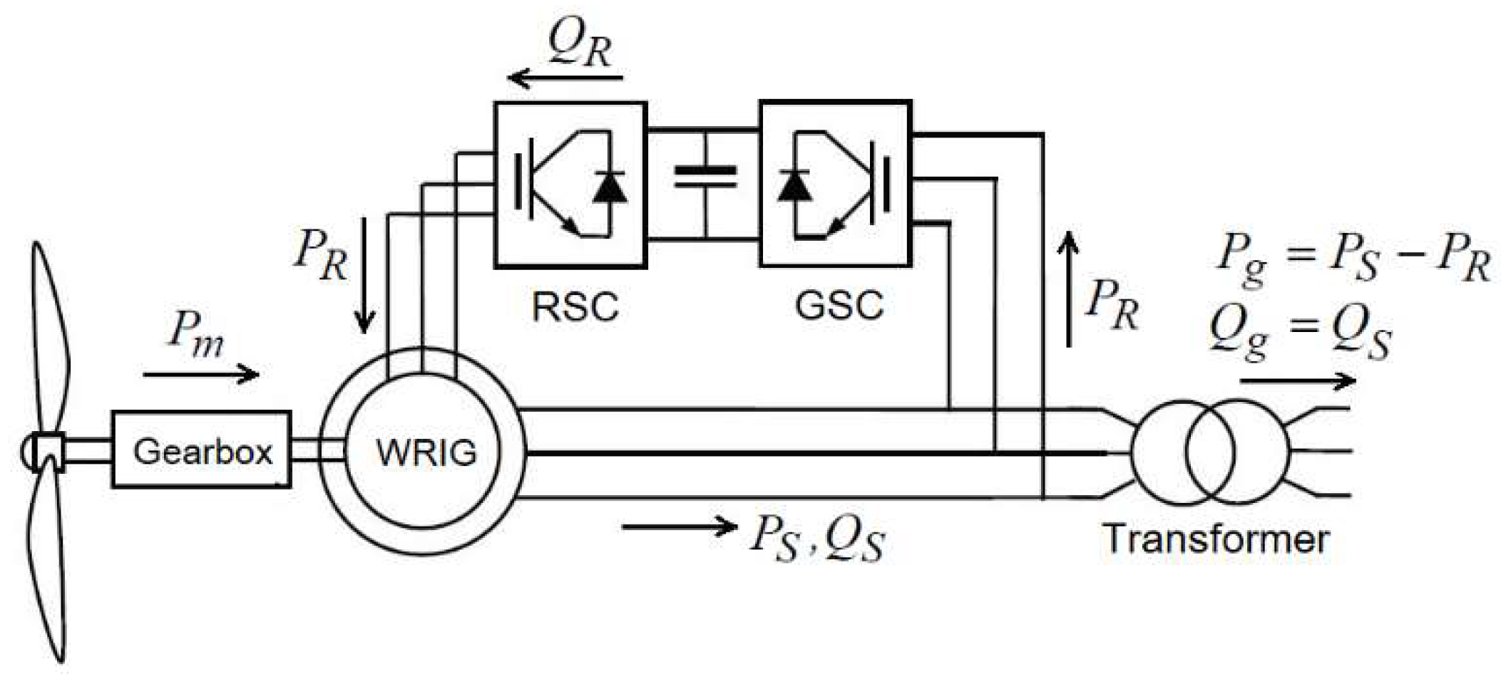
3. DFIG Structure and Power Calculations
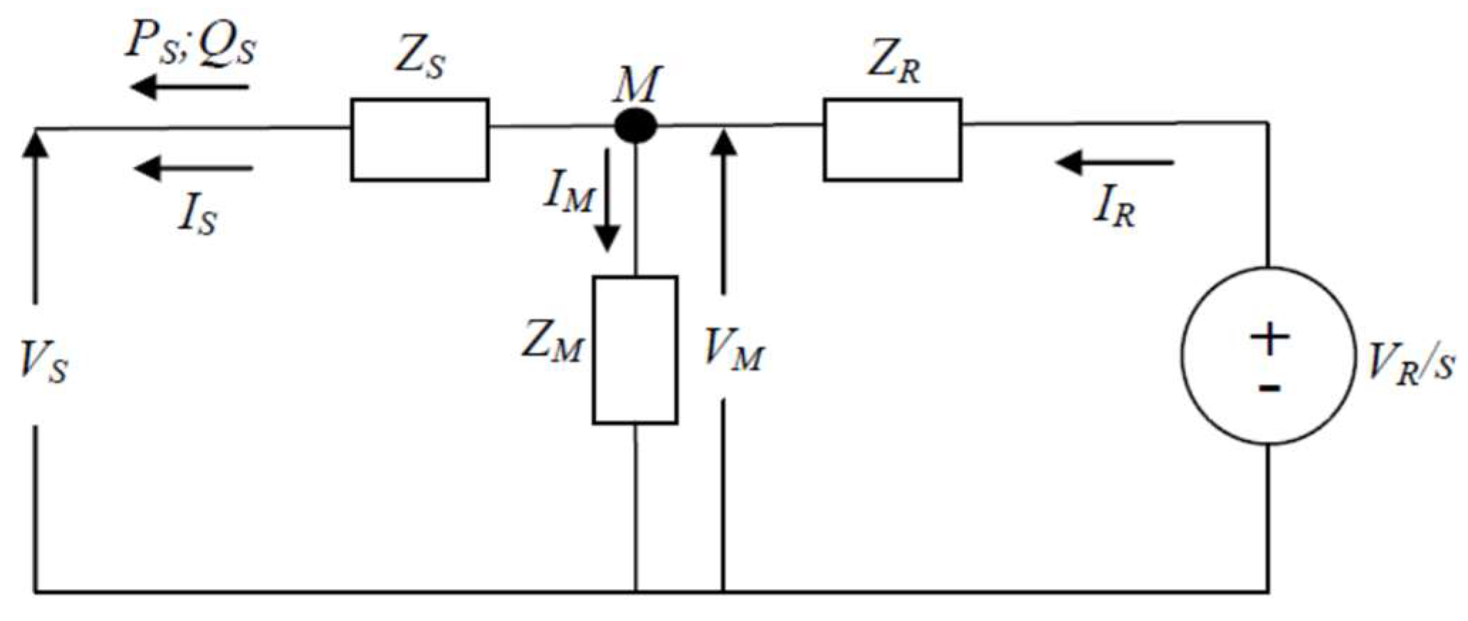
3.1. DFIG Structure and Equivalent Circuit
| RS, XS | : | resistance, reactance of stator circuit |
| RR, XR | : | resistance, reactance of rotor circuit |
| Rc, Xm | : | resistance, reactance of core magnetic circuit |
3.2. Steady State Model of DFIG-Based WPP
| i = 1, 2, …, n | : | bus number |
| n | : | total number of buses |
| SGi = PGi + jQGi | : | power generation at bus i |
| SLi = PLi + jQLi | : | power load at bus i |
| Vi = |Vi|ejδi | : | voltage at bus i |
| Yij = |Yij|ejθij | : | element ij of admittance matrix |
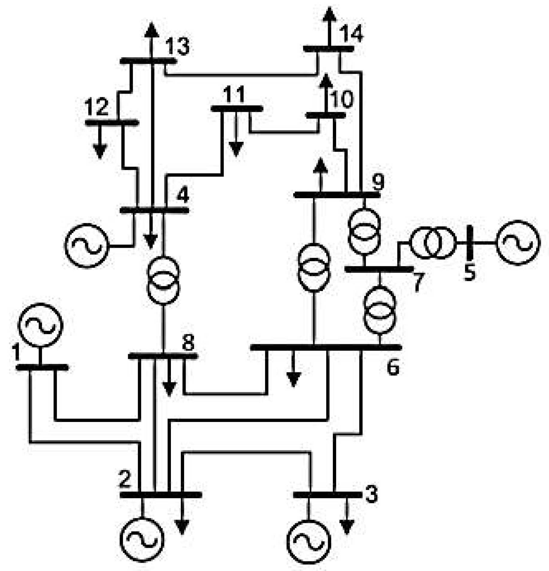
4. Case Study
4.1. Test System
4.2. WRIG Slip and Turbine Power Calculations
4.3. Aggregation of Wind Turbine Generator Units
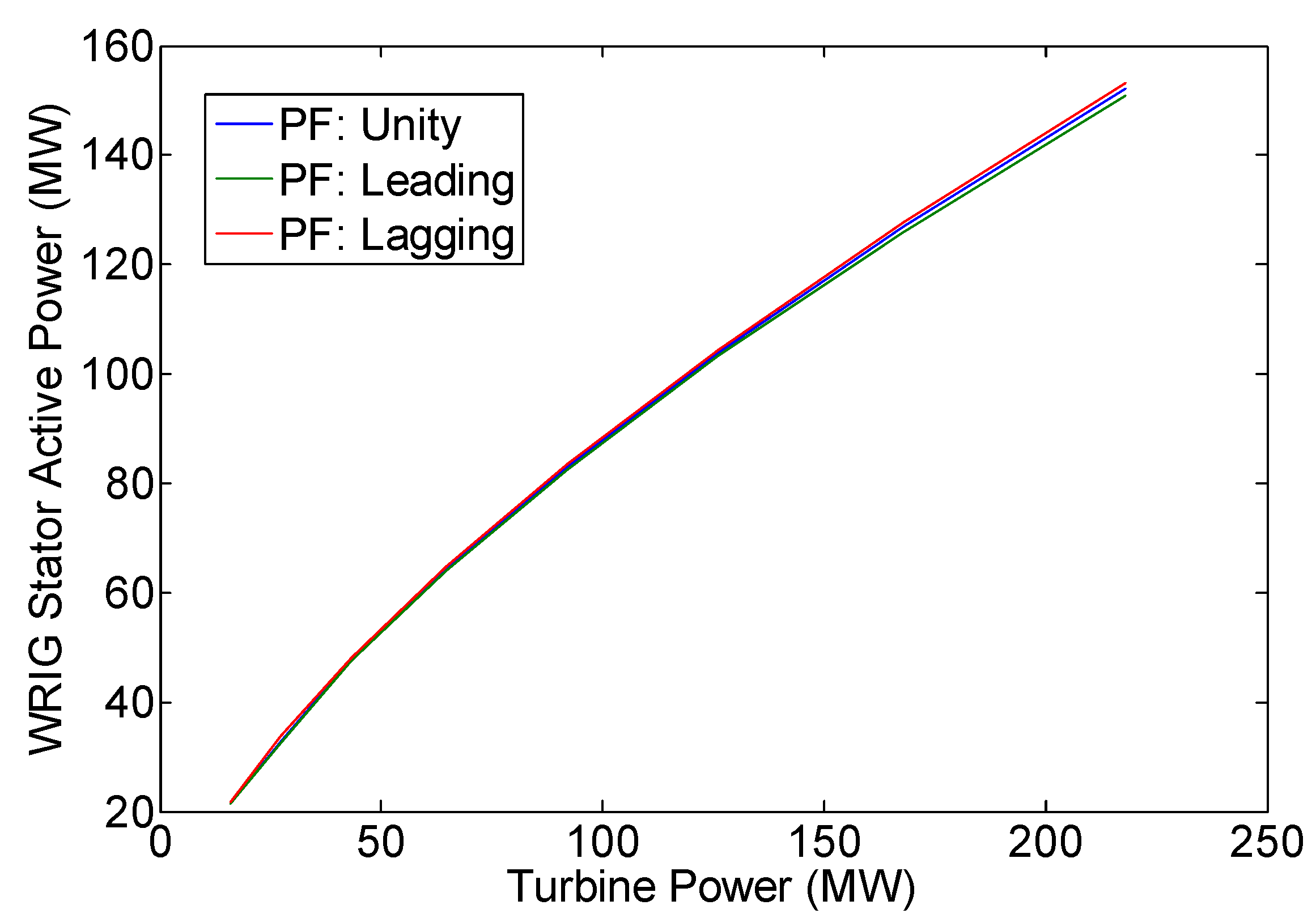
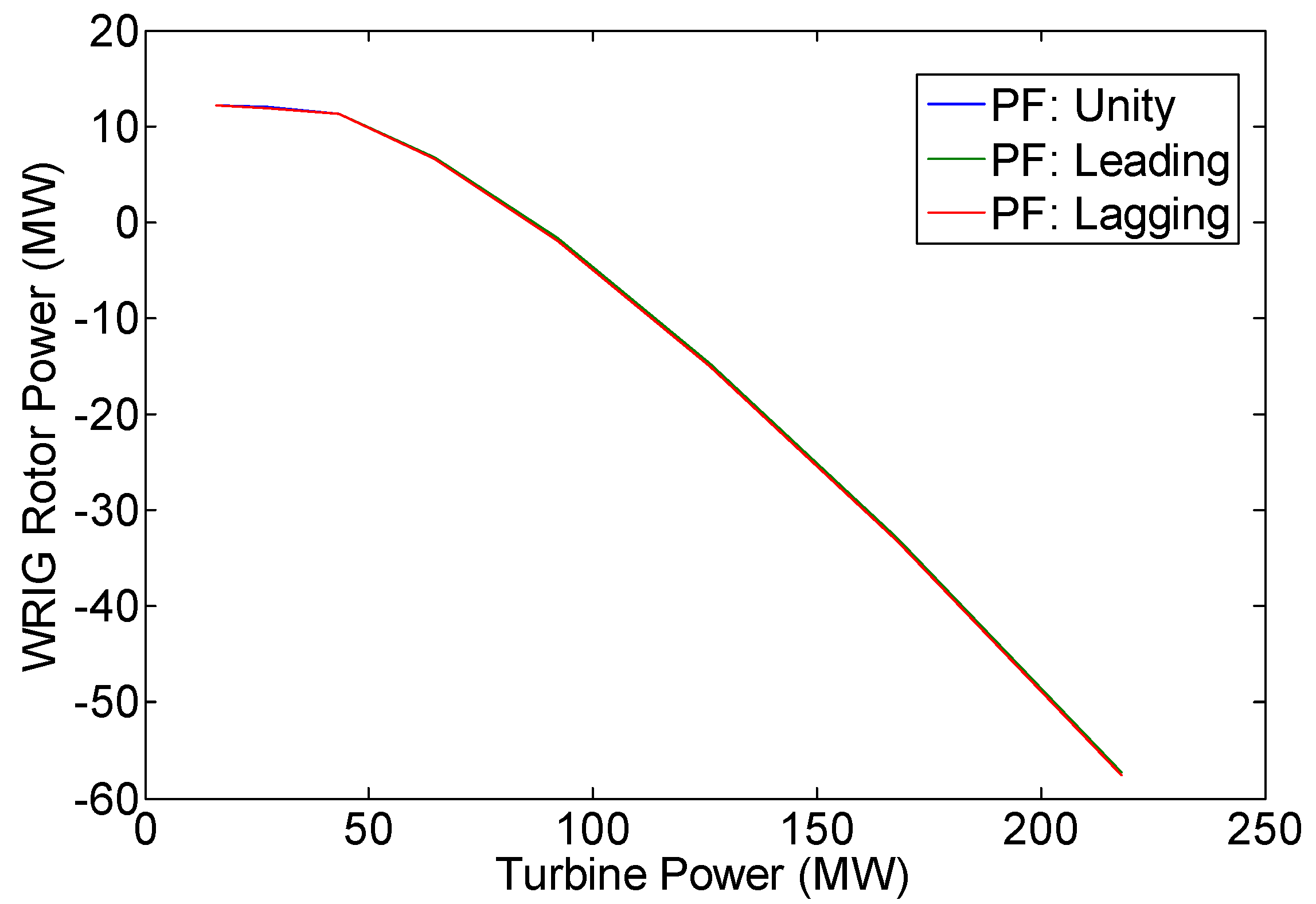
4.4. Load Flow Results and Discussion
5. Conclusions
Funding
Institutional Review Board Statement
Informed Consent Statement
Data Availability Statement
Conflicts of Interest
References
- Anaya-Lara, O.; Jenkins, N.; Ekanayake, J.B.; Cartwright, P.; Hughes, M. Wind Energy Generation: Modelling and Control; John Wiley & Sons. Ltd.: Chichester, UK, 2009. [Google Scholar]
- Ackermann, T. Wind Power in Power Systems; John Wiley & Sons. Ltd.: Chichester, UK, 2012. [Google Scholar]
- Li, H.; Chen, Z. Overview of different wind generator systems and their comparisons. IET Renew. Power Gener. 2008, 2, 123–138. [Google Scholar] [CrossRef] [Green Version]
- Babu, N.R.; Arulmozhivarman, A. Wind energy conversion system—A technical review. J. Eng. Sci. Technol. 2013, 8, 493–507. [Google Scholar]
- Haque, M.H. Evaluation of power flow solutions with fixed speed wind turbine generating systems. Energy Convers. Manag. 2014, 79, 511–518. [Google Scholar] [CrossRef]
- Haque, M.H. Incorporation of fixed speed wind turbine generators in load flow analysis of distribution systems. Int. J. Renew. Energy Technol. 2015, 6, 317–324. [Google Scholar] [CrossRef]
- Wang, J.; Huang, C.; Zobaa, A.F. Multiple-node models of asynchronous wind turbines in wind farms for load flow analysis. Electr. Power Compon. Syst. 2015, 44, 135–141. [Google Scholar] [CrossRef] [Green Version]
- Feijoo, A.; Villanueva, D. A PQ model for asynchronous machines based on rotor voltage calculation. IEEE Trans. Energy Convers. 2016, 31, 813–814, Correction in IEEE Trans. Energy Convers. 2016, 31, 1228. [Google Scholar] [CrossRef]
- Ozturk, O.; Balci, M.E.; Hocaoglu, M.H. A new wind turbine generating system model for balanced and unbalanced distribution systems load flow analysis. Appl. Sci. 2018, 8, 502. [Google Scholar]
- Gianto, R.; Khwee, K.H.; Priyatman, H.; Rajagukguk, M. Two-port network model of fixed-speed wind turbine generator for distribution system load flow analysis. Telkomnika 2019, 17, 1569–1575. [Google Scholar] [CrossRef]
- Gianto, R. Steady state model of wind power plant for load flow study. In Proceedings of the 2020 International Seminar on Intelligent Technology and Its Applications (ISITIA 2020), Surabaya, Indonesia, 22–23 July 2020; pp. 119–122. [Google Scholar]
- Gianto, R. T-circuit model of asynchronous wind turbine for distribution system load flow analysis. Int. Energy J. 2019, 19, 77–88. [Google Scholar]
- Gianto, R.; Khwee, K.H. A new T-circuit model of wind turbine generator for power system steady state studies. Bull. Electr. Eng. Inform. 2021, 10, 550–558. [Google Scholar] [CrossRef]
- Dadhania, A.; Venkatesh, B.; Nassif, A.B.; Sood, V.K. Modeling of doubly fed induction generators for distribution system power flow analysis. Electr. Power Energy Syst. 2013, 53, 576–583. [Google Scholar] [CrossRef]
- Ju, Y.; Ge, F.; Wu, W.; Lin, Y.; Wang, J. Three-phase steady-state model of DFIG considering various rotor speeds. IEEE Access 2016, 4, 9479–9948. [Google Scholar] [CrossRef]
- Kumar, V.S.S.; Thukaram, D. Accurate modeling of doubly fed induction based wind farms in load flow analysis. Electr. Power Syst. Res. 2018, 15, 363–371. [Google Scholar]
- Li, S. Power flow modeling to doubly-fed induction generators (DFIGs) under power regulation. IEEE Trans. Power Syst. 2013, 28, 3292–3301. [Google Scholar] [CrossRef]
- Anirudh, C.V.S.; Seshadri, S.K.V. Enhanced modeling of doubly fed induction generator in load flow analysis of distribution systems. IET Renew. Power Gener. 2021, 15, 980–989. [Google Scholar]
- Gianto, R. Steady state model of DFIG-based wind power plant for load flow analysis. IET Renew. Power Gener. 2021, 15, 1724–1735. [Google Scholar] [CrossRef]
- Gianto, R. Integration of DFIG-based variable speed wind turbine into load flow analysis. In Proceedings of the 2021 International Seminar on Intelligent Technology and Its Applications (ISITIA 2021), Virtual, 21–22 July 2021; pp. 63–66. [Google Scholar]
- Gianto, R. Steady state load flow model of DFIG-based wind turbine in voltage control mode. In Proceedings of the 3rd International Conference on High Voltage Engineering and Power Systems (ICHVEPS 2021), Bandung, Indonesia, 5–6 October 2021; pp. 232–235. [Google Scholar]
- Gianto, R. Constant voltage model of DFIG-based variable speed wind turbine for load flow analysis. Energies 2021, 14, 8549. [Google Scholar] [CrossRef]
- Akhmatov, V. Induction Generators for Wind Power; Multi-Science Publishing Co. Ltd.: Brentwood, UK, 2007. [Google Scholar]
- Boldea, I. Variable Speed Generators; Taylor & Francis Group LLC: Roca Baton, FL, USA, 2005. [Google Scholar]
- Fox, B.; Flynn, D.; Bryans, L.; Jenkins, N.; Milborrow, D.; O’Malley, M.; Watson, R.; Anaya-Lara, O. Wind Power Integration: Connection and System Operational Aspects; The Institution of Engineering and Technology: London, UK, 2007. [Google Scholar]
- Patel, M.R. Wind and Solar Power Systems; CRC Press LLC: Boca Raton, FL, USA, 1999. [Google Scholar]
- Gianto, R.; Khwee, K.H. A new method for load flow solution of electric power distribution system. Int. Rev. Electr. Eng. 2016, 11, 535–541. [Google Scholar] [CrossRef]
- Gianto, R. Trust-region method for load flow solution of three-phase unbalanced electric power distribution system. J. Electr. Comput. Eng. 2022, 2022, 5415300. [Google Scholar] [CrossRef]
- Pai, M.A. Computer Techniques in Power System Analysis; Tata McGraw- Hill Publishing Co. Ltd.: New Delhi, India, 1984. [Google Scholar]


| Bus Type | Equation(s) | Known Variables | Unknown Variables |
|---|---|---|---|
| Slack | (11) | |V| and δ = 0o | PG and QG |
| PV | (11) | PG and |V| | δ and QG |
| PQ | (11) | PG = QG = 0 | |V| and δ |
| WPP | (10) and (11) | , s, and Pm | |V|, δ, PG = Pg, QR, Re(IS) and Im(IS) |
| Line | Sending Bus | Receiving Bus | Series Impedance |
|---|---|---|---|
| 1 | 1 | 2 | 0.01938 + j0.05917 |
| 2 | 2 | 3 | 0.04699 + j0.19797 |
| 3 | 2 | 6 | 0.05811 + j0.17632 |
| 4 | 1 | 8 | 0.05403 + j0.22304 |
| 5 | 2 | 8 | 0.05695 + j0.17388 |
| 6 | 3 | 6 | 0.06701 + j0.17103 |
| 7 | 6 | 8 | 0.01335 + j0.04211 |
| 8 | 4 | 8 | j0.25202 |
| 9 | 6 | 7 | j0.20912 |
| 10 | 5 | 7 | j0.17615 |
| 11 | 6 | 9 | j0.55618 |
| 12 | 7 | 9 | j0.11001 |
| 13 | 9 | 10 | 0.03181 + j0.08450 |
| 14 | 4 | 11 | 0.09498 + j0.19890 |
| 15 | 4 | 12 | 0.12291 + j0.25581 |
| 16 | 4 | 13 | 0.06615 + j0.13027 |
| 17 | 9 | 14 | 0.12711 + j0.27038 |
| 18 | 10 | 11 | 0.08205 + j0.19207 |
| 19 | 12 | 13 | 0.22092 + j0.19988 |
| 20 | 13 | 14 | 0.17093 + j0.34802 |
| Bus | |V| | δ | Generation | Load | Note |
|---|---|---|---|---|---|
| 1 | 1.060 | 0 | - | 0 | Slack |
| 2 | 1.045 | - | 0.4 + j- | 0.217 + j0.127 | PV |
| 3 | 1.010 | - | j- | 0.942 + j0.190 | PV |
| 4 | 1.070 | - | j- | 0.112 + j0.075 | PV |
| 5 | 1.090 | - | j- | 0 | PV |
| 6 | - | - | 0 | 0.478 + j0.039 | PQ |
| 7 | - | - | 0 | 0 | PQ |
| 8 | - | - | 0 | 0.176 + j0.016 | PQ |
| 9 | - | - | 0 | 0.295 + j0.166 | PQ |
| 10 | - | - | 0 | 0.190 + j0.058 | PQ |
| 11 | - | - | 0 | 0.135 + j0.018 | PQ |
| 12 | - | - | 0 | 0.161 + j0.016 | PQ |
| 13 | - | - | 0 | 0.135 + j0.058 | PQ |
| 14 | - | - | 0 | 0.149 + j0.050 | PQ |
| Turbine | Blade length: 40 m Rated power: 3.0 MW Speed: Cut-in: 3 m/s; Rated: 14 m/s; Cut-out: 23 m/s |
| Gearbox | Ratio: 1/90 |
| Generator | Type: DFIG Rated power: 3.0 MW Pole pairs: 2 Voltage: 690 Volt Resistances/Reactances (in pu): RS = 1; XS = 10; RR = 1; XR = 10; Rc = 5000; Xm = 500 |
| Pad-Mount Transformer | Impedance (in pu): j5 |
| Vw (meter/s) | s | Pm (MW) | ΣPm (MW) |
|---|---|---|---|
| 5 | 0.4306 | 0.15780 | 15.78 |
| 6 | 0.3167 | 0.27270 | 27.27 |
| 7 | 0.2029 | 0.43300 | 43.30 |
| 8 | 0.0809 | 0.64630 | 64.63 |
| 9 | −0.0249 | 0.92020 | 92.02 |
| 10 | −0.1388 | 1.26230 | 126.23 |
| 11 | −0.2526 | 1.68010 | 168.01 |
| 12 | −0.3665 | 2.18120 | 218.12 |
| WRIG | RS,eq = 0.01; XS,eq = 0.10; RR,eq = 0.01; XR,eq = 0.10; Rc,eq = 50; Xm,eq = 5 |
| Pad-Mount Transformer | ZT,eq = 0.05 |
| ΣPm (MW) | Pg (MW) | Qg = QS (MVAR) | PS (MW) | PR (MW) |
|---|---|---|---|---|
| 15.78 | 9.4127 | 0 | 21.4955 | 12.0828 |
| 27.27 | 20.8045 | 0 | 32.8212 | 12.0167 |
| 43.30 | 36.6883 | 0 | 47.9329 | 11.2446 |
| 64.63 | 57.8139 | 0 | 64.4185 | 6.6046 |
| 92.02 | 84.9318 | 0 | 83.0831 | −1.8487 |
| 126.23 | 118.7934 | 0 | 103.9265 | −14.8669 |
| 168.01 | 160.1414 | 0 | 126.9522 | −33.1892 |
| 218.12 | 209.7292 | 0 | 152.1444 | −57.5848 |
| ΣPm (MW) | QR (MVAR) | PLOSS (MW) | QLOSS (MVAR) |
|---|---|---|---|
| 15.78 | 63.6728 | 6.3673 | 63.6728 |
| 27.27 | 64.6551 | 6.4655 | 64.6551 |
| 43.30 | 66.1171 | 6.6117 | 66.1171 |
| 64.63 | 68.1608 | 6.8161 | 68.1608 |
| 92.02 | 70.8821 | 7.0882 | 70.8821 |
| 126.23 | 74.3658 | 7.4366 | 74.3658 |
| 168.01 | 78.6861 | 7.8686 | 78.6861 |
| 218.12 | 83.9077 | 8.3908 | 83.9077 |
| ΣPm (pu) | Voltage (pu) | G1 to G5 Outputs | Line Losses | ||
|---|---|---|---|---|---|
| MW | MVAR | MW | MVAR | ||
| 15.78 | 1.0160 | 941.7797 | 479.5449 | 54.1924 | 235.6449 |
| 27.27 | 1.0196 | 928.6547 | 470.9905 | 52.4592 | 227.0905 |
| 43.30 | 1.0243 | 910.5415 | 459.8925 | 50.2298 | 215.9925 |
| 64.63 | 1.0301 | 886.7778 | 446.5797 | 47.5917 | 202.6797 |
| 92.02 | 1.0368 | 856.8002 | 431.8180 | 44.7320 | 187.9180 |
| 126.23 | 1.0440 | 820.1648 | 416.8994 | 41.9582 | 172.9994 |
| 168.01 | 1.0512 | 776.5829 | 403.7411 | 39.7243 | 159.8411 |
| 218.12 | 1.0575 | 725.9341 | 395.0049 | 38.6634 | 151.1049 |
| ΣPm (MW) | Pg (MW) | Qg = QS (MVAR) | PS (MW) | PR (MW) |
|---|---|---|---|---|
| 15.78 | 9.3484 | 3.0727 | 21.4447 | 12.0962 |
| 27.27 | 20.6617 | 6.7912 | 32.5085 | 11.8469 |
| 43.30 | 36.4350 | 11.9756 | 47.7337 | 11.2987 |
| 64.63 | 57.4122 | 18.8705 | 64.1035 | 6.6913 |
| 92.02 | 84.3374 | 27.7203 | 82.6185 | −1.7189 |
| 126.23 | 117.9556 | 38.7701 | 103.2733 | −14.6823 |
| 168.01 | 159.0028 | 52.2617 | 126.0661 | −32.9368 |
| 218.12 | 208.2259 | 68.4405 | 150.9748 | −57.2511 |
| ΣPm (MW) | QR (MVAR) | PLOSS (MW) | QLOSS (MVAR) |
|---|---|---|---|
| 15.78 | 67.3883 | 6.4316 | 64.3156 |
| 27.27 | 72.8742 | 6.6083 | 66.0830 |
| 43.30 | 80.6255 | 6.8650 | 68.6499 |
| 64.63 | 91.0488 | 7.2178 | 72.1783 |
| 92.02 | 104.5468 | 7.6826 | 76.8265 |
| 126.23 | 121.5143 | 8.2744 | 82.7441 |
| 168.01 | 142.3333 | 9.0072 | 90.0716 |
| 218.12 | 167.3817 | 9.8941 | 98.9412 |
| ΣPm (pu) | Voltage (pu) | G1 to G5 Outputs | Line Losses | ||
|---|---|---|---|---|---|
| MW | MVAR | MW | MVAR | ||
| 15.78 | 1.0192 | 941.7856 | 476.2581 | 54.1341 | 235.4308 |
| 27.27 | 1.0265 | 928.6796 | 463.7667 | 52.3413 | 226.6579 |
| 43.30 | 1.0364 | 910.6097 | 447.2361 | 50.0447 | 215.3117 |
| 64.63 | 1.0489 | 886.9239 | 426.7644 | 47.3361 | 201.7349 |
| 92.02 | 1.0641 | 857.0613 | 402.8550 | 44.3987 | 186.6753 |
| 126.23 | 1.0818 | 820.5608 | 376.4609 | 41.5164 | 171.3310 |
| 168.01 | 1.1016 | 777.0774 | 349.0208 | 39.0802 | 157.3825 |
| 218.12 | 1.1232 | 726.3667 | 322.4684 | 37.5925 | 147.0090 |
| ΣPm (MW) | Pg (MW) | Qg = QS (MVAR) | PS (MW) | PR (MW) |
|---|---|---|---|---|
| 15.78 | 9.4768 | −3.1149 | 21.5466 | 12.0698 |
| 27.27 | 20.9437 | −6.8838 | 33.7330 | 12.7893 |
| 43.30 | 36.9277 | −12.1376 | 48.1273 | 11.1996 |
| 64.63 | 58.1782 | −19.1222 | 64.7191 | 6.5409 |
| 92.02 | 85.4413 | −28.0832 | 83.5136 | −1.9278 |
| 126.23 | 119.4594 | −39.2644 | 104.5087 | −14.9507 |
| 168.01 | 160.9575 | −52.9042 | 127.7034 | −33.2541 |
| 218.12 | 210.6572 | −69.2397 | 153.0724 | −57.5848 |
| ΣPm (MW) | QR (MVAR) | PLOSS (MW) | QLOSS (MVAR) |
|---|---|---|---|
| 15.78 | 59.9176 | 6.3032 | 63.0324 |
| 27.27 | 56.3795 | 6.3263 | 63.2634 |
| 43.30 | 51.5852 | 6.3723 | 63.7228 |
| 64.63 | 45.3961 | 6.4518 | 64.5183 |
| 92.02 | 37.7034 | 6.5787 | 65.7866 |
| 126.23 | 28.4412 | 6.7706 | 67.7056 |
| 168.01 | 17.6207 | 7.0525 | 70.5249 |
| 218.12 | 5.3885 | 7.4628 | 74.6282 |
| ΣPm (pu) | Voltage (pu) | G1 to G5 Outputs | Line Losses | ||
|---|---|---|---|---|---|
| MW | MVAR | MW | MVAR | ||
| 15.78 | 1.0128 | 941.7820 | 482.9034 | 54.2587 | 235.8885 |
| 27.27 | 1.0125 | 928.6695 | 478.4409 | 52.6131 | 227.6571 |
| 43.30 | 1.0118 | 910.5955 | 473.1122 | 50.5232 | 217.0747 |
| 64.63 | 1.0103 | 886.9325 | 467.6194 | 48.1106 | 204.5972 |
| 92.02 | 1.0074 | 857.1856 | 463.2116 | 45.6270 | 191.2284 |
| 126.23 | 1.0025 | 821.0420 | 461.8678 | 43.5014 | 178.7034 |
| 168.01 | 0.9940 | 778.4596 | 466.5709 | 42.4171 | 169.7667 |
| 218.12 | 0.9801 | 729.7969 | 479.8147 | 41.4541 | 168.6751 |
Publisher’s Note: MDPI stays neutral with regard to jurisdictional claims in published maps and institutional affiliations. |
© 2022 by the author. Licensee MDPI, Basel, Switzerland. This article is an open access article distributed under the terms and conditions of the Creative Commons Attribution (CC BY) license (https://creativecommons.org/licenses/by/4.0/).
Share and Cite
Gianto, R. Constant Power Factor Model of DFIG-Based Wind Turbine for Steady State Load Flow Studies. Energies 2022, 15, 6077. https://doi.org/10.3390/en15166077
Gianto R. Constant Power Factor Model of DFIG-Based Wind Turbine for Steady State Load Flow Studies. Energies. 2022; 15(16):6077. https://doi.org/10.3390/en15166077
Chicago/Turabian StyleGianto, Rudy. 2022. "Constant Power Factor Model of DFIG-Based Wind Turbine for Steady State Load Flow Studies" Energies 15, no. 16: 6077. https://doi.org/10.3390/en15166077
APA StyleGianto, R. (2022). Constant Power Factor Model of DFIG-Based Wind Turbine for Steady State Load Flow Studies. Energies, 15(16), 6077. https://doi.org/10.3390/en15166077