Article

Effects of Confining Pressure and Hydrostatic Pressure on the Fracturing of Rock under Cyclic Electrohydraulic Shock Waves

College of Petroleum Engineering, China University of Petroleum-Beijing, Beijing 102249, China
*
Author to whom correspondence should be addressed.
Energies 2022, 15(16), 6032; https://doi.org/10.3390/en15166032
Submission received: 21 July 2022 / Revised: 10 August 2022 / Accepted: 17 August 2022 / Published: 19 August 2022

Abstract

:
For an array of applications of the high voltage pulse discharge technology in reservoir stimulations and to gain a deeper understanding of the fractures mechanism of deep well rock under cyclic electrohydraulic shock waves (EHSWs), the effect of confining pressure and hydrostatic pressure on the fracturing of rock under EHSWs are investigated in this paper. Firstly, a two-dimensional (2D) water-explosive numerical model is built to match the computed peak pressure of the EHSW with that obtained by the empirical formula by tuning the relevant parameters, based on the equivalent method of EHSWs. Then, a rock model is established to obtain the stress distribution under static loads. Subsequently, the water-explosive model is coupled with the rock model to obtain the stress distribution under static and dynamic loads. In addition, based on this coupling model, the influences of confining pressure and hydrostatic pressure on circumferential stress, radial stress in the rock and the fracturing of rock around the wellbore are discussed. Finally, two improvement measures (increasing discharge energy and changing loading mode) are proposed to acquire greater fracture density based on intensive numerical simulations. The results show that the increase in hydrostatic pressure is beneficial to the crack formation and development, whereas confining pressure is harmful. Moreover, the inhibitory effect of confining pressure on crack formation is greater than the promotion effect of hydrostatic pressure on crack formation. Increasing the discharge energy can effectively promote the development of the number and length of main cracks. Under four repetitive loading modes with the same total discharge energy (1.36 × 15 kJ), the greatest fracture density can be obtained by using repetitive loading mode with a gradually decreasing mode of discharge energy (first level: 2 times (1.36 × 5 kJ); second level: 5 times (1.36 × 1 kJ)).

1. Introduction

For practical applications, high voltage pulse discharge technology has received a lot of attention. It may be widely used for a variety of things, such as electrohydraulic forming [1], acoustic sources in medical or sonar applications [2,3], oil/gas well stimulation [4] and so on. In particular, in the development of tight oil and gas reservoirs, this technology may be considered as an alternative to hydraulic fracturing of oil and gas reservoirs.
Normally, hydraulic fracturing is the most widely used technology in reservoir stimulation [5]. During the implementation of hydraulic fracturing, the fluid (generally called fracturing fluid) drives fractures and carries proppant into fractures to keep them conductive after relieving fluid pressure. After fractures are generated and extended from a borehole into rock formation, the oil and gas can flow from the formation into the borehole through the fracture with much less resistance. However, conventional quasi-static hydraulic fracturing cannot generate enough fractures in a rather large volume surrounding the borehole. As a result, well production usually decreases noticeably after a period [6]. Moreover, due to its use of a large quantity of chemical substances, it is considered risk of pollution to the environment.
Differently from hydraulic fracturing, electrohydraulic shock wave fracturing is a dynamic progress of fracture initiation and propagation by the electrohydraulic shock wave (EHSW). The EHSW is a kind of powerful mechanical wave with high pressure and high energy density front [7]. Under the action of repetitive EHSWs induced by high voltage pulse discharge, multiple fractures are generated in the bulk material surrounding the borehole, which increases the bulk material’s permeability over a reasonably large volume and then stimulates oil and gas production. Although both charge explosion [8] and electrical explosion of wires [9] can also form powerful shock waves, the cyclic loading of repetitive shock wave cannot be formed due to the manual installation of explosion source. However, benefiting from the simplicity and durability of the EHSW generator, repetitive and controllable shock waves can be generated by adjusting the electrical parameters of the discharge circuit.
Some scholars have built relevant experimental setups for the EHSW generation and conducted physical simulation experiments. From the perspectives of crack distribution, permeability, porosity and so on, the damage characteristics of the EHSW to samples have been analyzed by X-ray computer tomography, mercury intrusion porosimetry, ultrasonic testing, etc. [4,6,10,11,12]. The above studies have shown that dynamic loads of EHSWs could effectively improve hole clogging and create and extend cracks.
Although abundant research results have been obtained through experiments, the following problems still exist. (1) It is difficult to simulate the formation environment on the ground due to limitations of experimental conditions (2) The cumulative damage mechanism of the sample subjected to the repetitive dynamic loads of EHSWs is not revealed. (3) It is difficult to clearly observe the crack formation and propagation inside the sample for building the quantitative relationship between crack numbers and impact numbers. (4) The experiment is expensive.
To cope with the problems above, the numerical simulation is an important method to study the electrohydraulic shock wave fracturing mechanism and optimize repetitive loading modes. However, due to the immaturity of the electrohydraulic breakdown theory and the lack of effective diagnosis methods for plasma channel parameters [13], few commercial numerical simulation software solutions can simulate the whole process of electrohydraulic discharge. Based on the experimental data, some scholars used the discrete element software Particle Flow Code (PFC) to simulate the electrohydraulic discharge fracturing process and achieved good simulation results [14,15], but did not consider the influences of confining pressure and hydrostatic pressure on fracture development. Moreover, the stress wave can only be imported artificially in PFC, which does not sufficiently describe the interaction process between the EHSW and the sample. The ANSYS/LS-DYNA, as commercial finite element software for explicit dynamics, is widely used in the field of explosions and shocks. It can effectively simulate the shock wave propagation and the crack generation [16,17]. Although the development process of a plasma leader is not able to be simulated in ANSYS/LS-DYNA, an equivalent method is proposed to indirectly simulate the formation and propagation of the EHSW in this paper.
In this study, a two-dimensional (2D) water-explosive numerical model was built to match the computed peak pressure of the EHSW with that obtained by the empirical formula by tuning the relevant parameters, based on the equivalent method of EHSWs. Then, a rock model was established to analyze the stress distribution under static loads. Subsequently, the water-explosive model was coupled with the rock model to analyze the stress distribution under static and dynamic loads. In addition, based on this coupling model, the influences of confining pressure and hydrostatic pressure on circumferential stress, radial stress in the rock and the fracturing of rock around the wellbore were considered. Finally, improvement measures were put forward to achieve the greater fracture density. The flowchart of the research process in this paper is shown in Figure 1. All in all, this paper provides an indirect method with which to simulate electrohydraulic shock wave fracturing based on ANSYS/LS-DYNA. The stress distribution, damage distribution and crack pattern of rock under confining pressure and hydrostatic pressure are obtained, and the fracturing effect is described and quantitatively analyzed. It is beneficial to improve the understanding of the mechanism of the fracture generation and growth in the rock under the coupled static–dynamic loads.
In order to make the structure of the article clearer, this paper’s remaining sections are structured as follows. The following is found in Section 2: methods used in the numerical simulation and model materials. In Section 3, numerical models are established and calculated; then, the stress distribution, damage distribution and crack pattern in the rock are obtained; the influences of hydrostatic pressure and confining pressure on those are analyzed. In Section 4, improvement measures are put forward to achieve the greater fracture density. In Section 5, conclusions are made.

2. Descriptions of Simulation Methods and Material Parameters

2.1. Equivalent Method of EHSWs

There are two methods to simulate the propagation process of the EHSW based on ANSYS/LS-DYNA. One is to treat the plasma channel detonation as the charge explosion [18,19], and the other is to treat the plasma channel as ideal gas [1]. For the former equivalent method, though the physical and chemical processes of generating shock waves are different, both can produce shock waves with large peak pressures and narrow wave widths. In reference [18], the combustion energy of the TNT explosive was equal to the deposition energy of electrohydraulic discharge, determining the TNT explosive mass. However, the calculated peak pressure of the shock wave based on underwater explosion is often larger than that based on actual experimental measurement. For the latter equivalent method, though it can reflect the physical state change process in the later stage of the electrohydraulic discharge plasma channel, how to determine the time of adiabatic expansion and the radius of the plasma channel at the moment of adiabatic expansion is very difficult. (The electric energy input to the plasma channel is equal to the energy output from the plasma channel due to radiation and conduction, and the plasma channel meets the adiabatic expansion condition [20].) Through a trial calculation, the EHWS peak pressure calculated by using the parameters in reference [1] is one or two orders of magnitude smaller than that calculated by Formula (1), and the waveform is much wider. By comparing both methods, the former equivalent method will be used to simulate the propagation process of the EHWS for its simplicity and accuracy.
Since the peak pressure of the shock wave is one of the important factors by which to judge the impact damage, the peak pressure of the shock wave is taken as the equivalent criterion. In other words, the peak pressure of the EHSW is equal to the peak pressure of TNT charge in the same environment, at the same distance, as much as possible. In order to achieve this purpose, we must first know the peak pressure attenuation law of the EHSW [21] and that of underwater explosion shock wave [22]. The correlation equation is as follows:
P dm = 9000 R d E B θ
E B = 1 2000 C U B 2
P bm = 53.1 Q 1 / 3 R b 1.13
where Pdm is the peak pressure generated by high voltage pulse discharge, bar; Rd is the distance from the discharge gap center, mm; EB is the discharge energy at the moment of breakdown, kJ; θ is the energy attenuation exponent, and the value of θ is 0.35 in reference [21]; C is the pulse energy storage capacitor value, μF; UB is the electrode breakdown voltage, kV; Pbm is the peak pressure of the shock wave generated by underwater explosion, MPa; Q is the mass of the explosive, kg; Rb is the distance from the explosive center, m.
Known from Equations (1)–(3), Pdm depends on EB and Rd, and Pbm depends on Q and Rb. Moreover, the attenuation exponents of peak pressure with the shock wave propagation distance are inconsistent, which are −1 and −1.13, respectively. These differences between Equations (1) and (3) make it difficult to effectively simulate the attenuation law of the peak pressure of the EHSW by regarding the plasma channel detonation as the charge explosion in water. Fortunately, the numerical simulation parameters, such as element size, the first-order artificial viscosity coefficient and charge radius, can be artificially modified to change the peak pressure and waveform of the shock wave in ANSYS/LS-DYNA [23], which provides a possibility that the peak pressure calculated by numerical simulation is as equal to the value calculated by Equation (3), as is possible within the effective action range of the shock wave.

2.2. Arbitrary Lagrangian–Eulerian Formulation

When the electric energy is injected into both ends of the electrode of the high-voltage pulse generator, the EHSW forms and propagates in the wellbore filled with a liquid medium. When the EHSW reaches the liquid-solid interface, reflection and transmission occurs. The transmitted wave continues to propagate in rock. In the process above, the rock subjected to the EHSW undergoes large deformation. When the numerical method is applied to solve the problem of large deformation, the element mesh easily becomes distorted, and hence the calculation is easy to terminate. The Eulerian formulation and arbitrary Lagrangian–Eulerian (ALE) formulation in ANSYS/LS-DYNA can be used to solve nonlinear dynamic problems with large deformation. The ALE multi-material formulation allows the finite element mesh to move independently from the material flow, and each element in the mesh contains a mixture of two or more different materials [24]. Compared with the Eulerian formulation, the element mesh position can be appropriately adjusted according to the defined parameters, so that the mesh will not be seriously distorted. In this study, the ALE method was employed as a fluid–structure interaction (FSI) method to facilitate the coupling interaction between explosive flow and solid material.

2.3. Simulation of Cumulative Damage

During an electrohydraulic shock wave fracturing operation, multiple charging and discharging cycles are often carried out, leading to repetitive EHSWs forming and acting on the rock. Every time acting on the sample, EHSW causes a certain degree of damage to the rock. Furthermore, cumulative damage would occur to the sample under the action of repetitive EHSWs. In order to simulate this whole process based on ANSYS/LS-DYNA, it is necessary to use the restart analysis technology of ANSYS/LS-DYNA. This technology can divide a complete analysis process into multiple stages. There are three types of restart analysis: simple restart, small restart and full restart. Full restart, among them, needs to be carried out when a large number of modifications are made to the original calculation model, such as adding new materials and parts, adding new contact definitions, changing the definitions of curves and changing some control parameters. In this study, full restart was used to achieve two purposes: one was to supply new explosive charge after the interaction between the rock and the shock wave generated by the last charge explosion. The other was that the deformation, stress, damage and other relevant data of the rock calculated before were inherited as the initial conditions for the next stage. It is worth noting that the inheritance of related data was achieved through the keyword *STRESS-INITIALIZATION-{OPTION}. Only when this keyword is included in the calculation file could the full restart be invoked in ANSYS/LS-DYNA.

2.4. Material Models

2.4.1. Water

Since water is strongly compressed during the formation of the EHSW, an equation of state (EOS) fit for high-pressure conditions should be used. The Mie–Grüneisen equation of state can better describe the thermodynamic behavior of water when suffering the impacting load. The equation is as follows [25,26]:
P = ρ 0 c 2 μ 1 + 1 γ 0 2 μ γ 2 μ 2 1 S 1 1 μ S 2 μ 2 μ + 1 S 3 μ 3 μ + 1 2 2 + γ 0 + α μ E 0
When the fluid is in a negative pressure state, it can be expressed as:
P = ρ 0 c 2 μ + γ 0 + α μ E 0
where E0 is the internal energy per initial volume; c is the intercept of the vsvp curve; S1, S2 and S3 are the unitless coefficients of the slope of the vsvp curve; γ0 is the unitless Gruneisen gamma; ρ0 is the initial density; α is the first-order volume correction to γ0; and μ = ρ/ρ0 − 1. The chosen values of each parameter were as follows: ρ0 = 1025 kg/m3, c = 1480 m/s; S1 = 2.56, S2 = −1.986, S3 = 1.2268, γ0 = 0.4934, V0 = 1, α = 0, E0 = 2.026 bar.

2.4.2. TNT

In order to successfully use the equivalent method of EHSWs, a suitable explosive model is required. In this study, TNT charge was modeled as a high explosive. An equation of state known as Jones–Wilkins–Lee (JWL) was applied to describe the pressure generated by chemical energy in an explosion. It can be written in the form [27]:
p = A   1 ω / R 1 V   e R 1 V + B   1 ω / R 2 V   e R 2 V + ω E / V
where p is pressure; V and E are the specific volume and the internal energy, respectively; A, B, R1, R2 and ω are material constants. The terms A and B are the pressure coefficients, R1 and R2 are the principal and secondary eigenvalues, respectively. ω is the fractional part of the normal Tait equation adiabatic exponent. e is a mathematical constant. The values of these parameters were as follows: A = 373.7 GPa, B = 3.74 GPa, R1 = 4.15, R2 = 0.90, ω = 0.35, Pcj = 21 GPa, ρ = 1630 kg/m3, E = 6.0 GJ/m3.

2.4.3. Rock

The response of the rock material under impact or blast loading is a complex non-linear and rate-dependent process. ANSYS/LS-DYNA software provides many constitutive models for choices in numerical simulation to characterize the dynamic behavior of rock materials under impact loading. Among those, the Riedel–Hiermaier–Thoma (RHT) model is adopted, which is particularly useful for modeling the dynamic behavior of concrete-like materials. Since rock and concrete are brittle materials with similar particle boundaries, voids, cracks, etc., they have the characteristics of strain hardening, damage softening and strain rate effects. Thus, the constitutive relation of concrete is employed to describe the mechanical behavior of rock under dynamic and static loading. This model consists of three strength surfaces: the elastic limit surface, failure surface and residual strength surface.
The failure surface, Y fail * P , θ ,   ε ˙ , is defined as a function of the normalized pressure P, the lode angle θ and strain rate:   ε ˙
Y fail * = Y TXC * P R 3 θ F RATE   ε ˙
Y TXC * P = A P * P spall * F RATE   ε ˙ N
where Y TXC * P is the compression meridian intensity; R3(θ) is introduced to describe the reduced strength on the shear and tensile meridian; F RATE   ε ˙ represents the dynamic increase factor (DIF) as a function of the strain rate; A is the failure surface constant; N is the failure surface index; P is the pressure normalized by fc, where fc is the material uniaxial compressive strength; P spall * is the normalized spall strength.
Strain rate effects are represented through increases in fracture strength with plastic strain rate. Two different terms can be used for compression and tension; linear interpolation is used in the intermediate pressure regime.
F RATE   ε ˙ =   ε ˙ / ε 0 ˙ α ,   f o r   P   >   f c / 3   c o m p r e s s i o n ε ˙   / ε 0 ˙ δ ,   f o r   P   <   f c / 3   t e n s i l e
where α is the compressive strain rate factor and δ is the tensile strain rate factor.
The elastic limit surface can be described as follows:
Y ela * = Y fail * F CAP P
where FCAP(P) is a function that limits the elastic deviatoric stresses under hydrostatic compression.
The residual failure surface can be described as
Y res * = B × P * M
where B is the residual failure surface constant and M is the residual failure surface exponent.
Damage is assumed to accumulate due to inelastic deviatoric straining (shear-induced cracking) using the relationships:
D = Δ ε PL / ε p failure
ε p failure = D 1 P * P spall * D 2
where ΔεPL is the equivalent plastic strain increment; D1 and D2 are damage constants; the damage factor D between 0 and 1 indicates the rock element damage ranges from undamaged material to fully damaged material.
Detailed formulation of the RHT dynamic damage model can be found in references [28,29]. The material parameters [29] adopted in the present work are based on the typical data for concrete material, as shown in Table 1.

3. Numerical Investigation

3.1. Model Simplification

The schematic diagram of three-dimensional (3D) electrohydraulic shock wave fracturing is shown in Figure 2. Under repeated EHSWs, cracks are formed in the rock formation around the wellbore and expand along the radial direction of the wellbore. This process actually involves a three-dimensional problem. The reasons for this are as follows: the shock waves generated between the discharge electrodes propagates outward in the form of a spherical surface, and they not only propagate in the horizontal section, but also propagate to the upper and lower parts of the horizontal section, which leads to the dynamic loads on the sidewall rock at different formation depths inconsistent. However, if a three-dimensional model were established for the next analysis, it could bring several difficulties. These difficulties are: (1) The complexity of the model increases. (2) The required computation time increases suddenly. (3). After several discharges, the restart analysis file is excessively large, resulting in insufficient storage resources. As a compromise, we still treated it as a two-dimensional (2D) plane strain problem, only analyzed the stress state of the rock in the horizontal section and reduced the size of the model to reduce the storage capacity.
Figure 3 shows the schematic diagram in the plane strain condition. This rock we subjected to the combination of dynamic and static loads, as shown in Figure 3a. The static loads (Figure 3b) included the confining pressure and hydrostatic pressure of magnitudes Pc and Ph, respectively. The dynamic loads (Figure 3c) were several discharge loads, which combined were Pd(t) generated by a TNT charge, which reached the interior surface of a circular wellbore. Therefore, when the coupled model was established, the static loads were applied to the rock first, and then the discharge loads were applied.

3.2. Parameter Calibration for the Peak Pressure of the EHSW

Before the establishment of the coupled model, the peak pressure generated by the equivalent method of EHSWs had to be matched with that calculated by Formula (1) by tuning the relevant parameters. Thus, the following steps were required:
(a)
Firstly, the required discharge parameters was determined. According to the typical discharge waveform provided in reference [15], the breakdown voltage is 30.1 kV and the capacitance is 3 μF, and then the discharge energy EB could be calculated to be 1.36 kJ according to the formula E B = 0.5 C U B 2 . By substituting EB into Formula (1), the peak pressure of shock waves under different distance from the charge center could be obtained.
(b)
Secondly, a 2D numerical model for a free-field underwater explosion was established. The 2D model was a cylinder with a single layer of solid mesh, as shown in Figure 4. The radius of the cylinder was 200 mm. All materials were modeled by the Euler grid. A non-reflecting boundary was applied at the truncating boundaries of the water.
(c)
Finally, a large number of trial calculations were carried out by adjusting the radius of the spherical charge and the first-order artificial viscosity coefficient, in order to match the numerical results as well as possible to the results calculated by Formula (1).
Figure 5 shows the comparison of numerical and empirical peak pressures. When the first-order artificial viscosity coefficient was set to 1.0 and the charge radius was set to 0.4 mm, numerical results for peak pressure of shock waves agreed well with the empirical results, which indicates that the coupling model is highly reliable and can be applied for subsequent calculation and analysis. Moreover, using the same steps, we also obtained the corresponding explosive radii of 0.55 and 0.63 mm at three times the discharge energy and five times the discharge energy, respectively, which can change the repetitive loading modes.

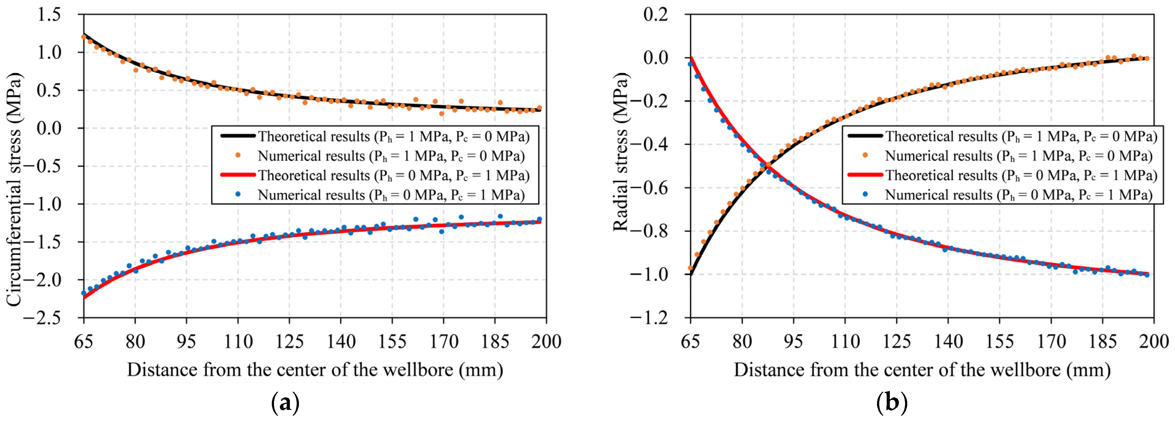
3.3. Stress Distributions under Static Loads

As analyzed in Section 3.1, static loads were applied to the rock prior to discharge loads. Therefore, we first applied a static load to the rock and then compared the numerical results with the theoretical formula to ensure that the static loads were successfully applied. The set-up of numerical model is shown in Figure 6. The radius of the center wellbore was 65 mm, and the radius of the outer circle was 200 mm. The pressures Ph and Pc were applied to the boundaries of the model, and then a static analysis was conducted with “dynain file” method [30] in ANSYS/LS-DYNA code. The purpose was to obtain the stress and displacement of each element induced by the initial pressure before discharge. At this stage, the TNT charge and water were not included in the model.
The complete solutions for stress distributions in polar coordinates in Figure 6 are [31]:
σ r r s = a 2 b 2 a 2 1 b 2 r 2 P h b 2 b 2 a 2 1 a 2 r 2 P c σ θ θ s = a 2 b 2 a 2 1 + b 2 r 2 P h b 2 b 2 a 2 1 + a 2 r 2 P c τ r θ s = 0
where a is the inner radius; b is the outer radius; r is the distance from the center of the wellbore; σ r r s and σ θ θ s are the radial and circumferential stresses, respectively; and τ r θ s is the shear stress.
After static loads are applied, the stress distribution in the rock before discharge can be obtained. The distributions of circumferential and radial stresses for two cases (case 1: Ph = 1 MPa, Pc = 0 MPa; case 2: Ph = 0 MPa, Pc = 1 MPa) are shown in Figure 7. It can be found in case 1 that the maximum circumferential stress is 1.218 MPa at the wellbore wall. The circumferential stress is tensile and the radial stress is compressive along the radial direction. However, in case 2, whether it is the circumferential stress or the radial stress, they both are in a state of compression. Particularly, the circumferential stress reaches a minimum value of −2.203 MPa due to stress concentration around the wellbore wall. In summary, the circumferential stress at the wellbore wall increases with the increase in Ph and decreases with the increase in Pc. Figure 8 shows the comparison of numerical and theoretical static stresses. It can be found that, regardless of the circumferential stress or radial stress, for case 1 and case 2, the numerical results are in good agreement with the theoretical results calculated by Formula (14), which indicates that the static load was successfully applied.

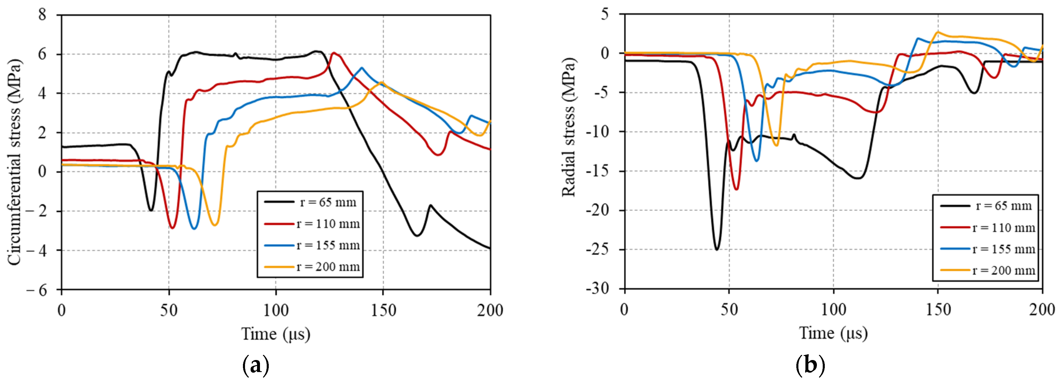
3.4. Stress Distributions under Static and Dynamic Loads

After the static load is successfully applied, the dynamic load can be added to the original model. The dynamic load comes from TNT charge in water, so the underwater explosion model and rock model need to be coupled. The coupled numerical model is shown in Figure 9. The numerical model of a free-field underwater explosion in Section 3.2 was extracted and combined with the rock model built in Section 3.3. The radii of the rock and water were 200 and 90 mm, respectively. The radius of the center wellbore was 65 mm. The fluid–solid coupling algorithm was applied. The non-reflecting boundary condition was set around the model to simulate an infinite rock medium. The discharge energy of 1.36 kJ was the same as that in Section 3.2, and the total number of discharges was 15.
Figure 10a shows the circumferential stress as a function of time for different locations (r = 65, 110, 155 and 200 mm respectively) when Pc = 0 MPa and Ph = 1 MPa. Figure 10b shows the results of the radial stress. Figure 10 indicates that the circumferential stress in the rock decreases from the prestress value to negative value and then increases to positive value. In other words, the circumferential stress changes from compressive stress tensile stress. The radial stress in the rock is negative most of the time, which implies that the rock is mainly subjected to compressive stress in the radial direction. Moreover, it can be found that the peak values of compressive stresses decrease quickly with the increasing distance from the center of the wellbore in Figure 10b; in Figure 10a, the time that the rock is in the tensile stress state in the circumferential direction is much longer than the time that the rock is in the state of compressive stress, which will cause a majority of cracks to grow in the radial direction. The above results are consistent with the historical curve of stress distributions in the rock obtained by the theoretical calculations in reference [32], indicating the credibility of the numerical results.

3.5. Effects of Confining Pressure and Hydrostatic Pressure on Circumferential and Radial Stresses

After obtaining the internal stress distribution of rock under static and dynamic loads, it is necessary to study the effect of hydrostatic pressure and confining pressure on circumferential stress and radial stress, which will be very helpful for the subsequent analysis of crack propagation.
Three cases were investigated as follows:
(a)
Case 1: Pc = 0 MPa; Ph = 0, 1, 2 or 3 MPa. This case is used to investigate the effect of Ph.
(b)
Case 2: Pc = 0, 1, 2 or 3 MPa; Ph = 0 MPa. This case is used to investigate the effect of Pc.
(c)
Case 3: Pc = Ph = 0, 1, 2 or 3 MPa. This case is used to investigate the degrees of influence of Ph and Pc.
Figure 11 shows the circumferential and radial stresses at different Ph and Pc when r = 155 mm. It can be found from Figure 11(a1,a2) that with the increase in hydrostatic pressure, the circumferential stress curve moves upward, which makes the tensile circumferential stress become larger. However, the position of the radial stress curve does not change much. As shown in Figure 11(b1,b2), with the increase in confining pressure, the radial stress and circumferential stress curves gradually move downward a certain distance, which indicates that the radial compressive stress becomes larger and the circumferential tensile stress becomes smaller. By comparing Figure 11(b1,b2,c1,c2), it can also be found that the change trends and shapes of the circumferential stress curve and the radial stress curve are roughly the same, which shows that hydrostatic pressure has less influence on the stress waveform than the confining pressure. In general, it can be seen in Figure 11 that an increase in the hydrostatic pressure will lead to an increase in the circumferential stress, and an increase in the confining pressure will do the opposite. Compared with the hydrostatic pressure, the changes in the radial stress and the circumferential stress are more sensitive to the confining pressure. The stress in the rock is the result of the linear superposition of the static loads and the dynamic loads outside the rock.

3.6. Effects of Confining Pressure and Hydrostatic Pressure on the Fracturing of the Rock

The ANSYS/LS-DYNA commercial software usually provides two methods to simulate the process of fracture initiation and propagation. (1) One is to use the damage distribution to describe the fracture. This method requires customization of the damage variable of the material or selecting a material model with the damage variable accounting for tensile and compressive failures in the material library. (2) The other is the element deletion method, requiring one to add a failure criterion to the corresponding material model through the keyword * MAT_ADD_EROSION. Elements will be deleted if the criteria are met. The deleted elements are connected to form cracks. Thus, the element size needs to be small enough to accurately describe the size and number of cracks. The former method was applied. The element with damage levels above 0.7 were blanked out to obtain the crack patter for three cases.
In order to investigate the effect of Ph on the damage evolution and fracturing in rock due to cyclic EHSWs, the damage distribution and crack pattern after 15 discharges are shown in Figure 12. It can be observed from Figure 12(a1,a2) that in the unstressed condition, a dense zone is created, as the rock at the wellbore wall is intensively shattered by the impact loading. The microcracks in this zone are relatively dense. Meanwhile, several main cracks emanate radially from the dense zone periphery under the tensile circumferential stress induced by cyclic impact loadings. These main cracks can also bifurcate along their paths of propagation in the fractured zone. As Ph increases, under the same discharge times, the damage distribution and crack pattern are roughly the same for the four conditions. However, when Pc = 0 MPa and Ph = 3 MPa, the number of main cracks is slightly greater and the damage area is slightly larger than in the other condition.
Figure 13 shows the variations in damage distribution and crack pattern with the increase in Pc. It can be seen, as the magnitude of Pc rises, under the same discharge times, the size of the dense zone gradually decreases and the extension and branching of radial cracks become suppressed. When Pc = 2 MPa and Ph = 0 MPa, there are no cracks formed. The results indicate the attenuation of the transmitted wave of EHSWs under the action of higher Pc will be aggravated, and the stress wave generated in rock is not enough to produce microcracks and main cracks.
Figure 14 shows the variations in damage distribution and crack pattern with the increase in Pc and Ph in the same increment. It can be observed that the larger Pc and Ph are, the smaller the size of the dense zone, the more difficult it is to form main cracks, the fewer the main cracks and the smaller the length of main cracks. However, by comparing Figure 14(b2,c2) and Figure 13(b2,c2), it can be found that an increase in Ph contributes to the formation of microcracks near the wellbore and main cracks in the fracture zone.
In order to provide quantitative insights into the effects of the Pc and Ph on the fracturing of rock under cyclic EHSWs, the following fracture density (η) was applied in this study to characterize the degree of crack development in various stress fields:
η = M f M t
where Mf is the number of the element of fractures, and Mt is total number of the element for rock.
Figure 15 shows the variation in fracture density under different Pc and Ph for three cases. It can be clearly seen in Figure 15 how Pc and Ph affect crack formation and development. As shown in Figure 15a, cracks form after three discharges for Ph = 1, 2 and 3 MPa, and after four discharges for Ph = 1 MPa, which indicates that Ph contributes to the earlier formation of cracks. The main reason for this phenomenon is that Ph makes the rock at the wellbore wall in a state of circumferential tension at the static load stage, and cracks are more likely to form under action of the tensile circumferential stress induced by cyclic impact loadings. Except for the case of Ph = 0 MPa, under the same discharge times, the greater the Ph, the greater the fracture density, which implies that the Ph is conducive to crack development.
It is worth noting that when Pc = 0 MPa and Ph = 1, 2 and 3 MPa, the growth trend of crack density with the number of discharges is different from that at Pc = Ph = 0 MPa. The reason for this may be the characterization of fracture density. Mf in the Formula (15) is the sum of tensile cracks and compression–shear cracks. The circumferential tensile state caused by Ph at the static loading stage, on the one hand, promotes the generation of tensile cracks, and on the other hand may inhibit the growth trend of compression–shear cracks in the dense zone. With the increase in the number of discharges, the growth trend of tensile cracks becomes larger and the growth trend of compressive-shear cracks becomes smaller, which makes the change in Mf more complicated, and then leads to the difference between fracture density when Pc = Ph = 0 MPa and that when Pc = 0 MPa and Ph = 1, 2 and 3 MPa.
The above analysis is based on Pc = 0 MPa. However, when confining pressure is applied, how does Ph affect the crack formation and development? By comparing variation in fracture density when Pc = 1 MPa and Ph = 0 MPa in Figure 15b with that at Pc = Ph = 1 MPa in Figure 15c, it can be found that cracks form after six discharges for the former and five for the latter. After 15 discharges, the fracture density for the former is 0.038, whereas that for the latter is 0.051, which indicates that under the condition of confining pressure, the increase in Ph makes cracks form earlier and the number of cracks greater. In general, Ph is beneficial to the crack formation and development.
It can be found from Figure 15b that cracks start to form after four discharges when Pc = Ph = 0 MPa, cracks start to form after six discharges when Pc = 1 MPa and Ph = 0 MPa, and no crack forms after 15 times discharges when Ph = 0 MPa and Pc = 1 or 2 MPa, which indicates that a high Pc inhibits the crack initiation and development. The reason for this result is that Pc makes the rock be under circumferential compression and radial compression at the static loading stage, which is not conducive to the formation of open cracks induced by circumferential tensile stress. As shown in Figure 15c, with the increases in Pc and Ph by the same increment, the formation of cracks is still suppressed, which indicates that the inhibitory effect of Pc on crack formation is greater than the promoting effect of Ph on crack formation.

4. Improvement Measures

4.1. Effects of the Discharge Energy

Through the analysis of the effects of confining pressure and hydrostatic pressure on the fracturing, it can be known that confining pressure has a strong inhibitory effect on crack initiation and growth. Unfortunately, in the actual working environment, formation rocks are often subject to high confining pressure. In order to promote crack formation and propagation, increasing the discharge energy is a relatively simple and common measure. Here we change the discharge energy by changing the radius of TNT charge. In Section 3.2, it is verified that when the discharge energies are 3 × 1.36 and 5 × 1.36 kJ, the corresponding radii of TNT charge are 0.55 and 0.63 mm, respectively. Therefore, damage distribution, crack pattern and crack density under different discharge energies when Pc = 1 MPa and Ph = 0 MPa are studied, as shown in Figure 16 and Figure 17.
It can be seen in Figure 16 that with the increase in single-discharge energy, the size of the dense zone and the number of main cracks in the fracture zone increase significantly. As shown in Figure 17, with a single-discharge energy of 1.36, 1.36 × 3 or 1.36 × 5 kJ, the corresponding number of discharges when cracks begin to form is 6, 3 or 2, respectively; and the corresponding crack densities after 15 discharges are 0.038, 0.142 and 0.202, respectively. The results show that the higher the discharge energy, the earlier the crack generation, and the greater the crack density under the same number of discharges.

4.2. Effects of Repetitive Loading Modes

In a practical application of high voltage pulse discharge technology, due to the constraints of the engineering environment and technical conditions, the discharge energy cannot be increased indefinitely, and the output discharge energy or discharge voltage often has an upper limit. Fortunately, the loading mode can be changed by adjusting the parameters of the out circuit to achieve multi-level adjustment of discharge energy. Therefore, when the total discharge energy is the same, the optimal discharge mode is explored to obtain the best fracturing effect.
As shown in Table 2, by changing the discharge energy EB, under the total discharge energy of 1.36 × 15 kJ, four test groups of discharge energy loading (Pc = 1 MPa, Ph = 0 MPa) were simulated. Among them, the single-discharge energy was increased in test groups 1 and 2; the discharge energy increased at each level in test group 3; and the discharge energy decreased at each level in the test group 4. The cumulative damage obtained from different test groups was extracted and summarized, as shown in Figure 18 and Figure 19.
As shown in Figure 19, by comparing test groups 1 and 4, and test groups 2 and 3, it can be found that the larger the discharge energy in the first level, the earlier the cracks are generated. By comparing test groups 1 and 3, and test groups 2 and 4, it can be found that the larger the single-discharge energy is, the larger the increment of the increase in fracture density after each discharge. Comparing four test groups, the loading mode of test group 4 achieved the greatest fracture density and the best fracturing effect.

5. Conclusions

In this study, the stress distributions in the rock, and damage distributions and crack patterns of rock subjected to cyclic electrohydraulic shock waves (15 impact loads) under different confining pressures (Pc = 0, 1, 2, 3 MPa) and hydrostatic pressures (Ph = 0, 1, 2, 3 MPa respectively) were investigated. In addition, two improvement measures (increasing discharge energy and changing loading mode) were proposed to acquire greater fracture density based on intensive numerical simulations. Through the research, findings and conclusions were obtained:
(1) Under cyclic electrohydraulic shock waves, the fracturing range of rock is divided into two zone: the dense zone and the fracture zone. In the dense zone, abundant microcracks are formed in the rock near the wellbore wall under compressive-shear stress. In the fracture zone, several main cracks are formed under the tensile circumferential stress.
(2) Overall, the increase in hydrostatic pressure is beneficial to crack formation and development, whereas confining pressure is detrimental. Moreover, the inhibitory effect of confining pressure on crack formation is greater than the promotion effect of hydrostatic pressure on crack formation.
(3) With higher discharge energy, the crack generation is earlier, and the crack density under the same number of discharges is greater. The larger the single-discharge energy is, the larger the increment in the crack number after each discharge. Under four repetitive loading modes with the same total discharge energy (1.36 × 15 kJ), the greatest fracture density can be obtained by using repetitive loading mode with gradually decreasing mode of discharge energy (first level: two times (1.36 × 5 kJ); second level: five times (1.36 × 1 kJ)).
(4) Based on the effects of various factors on the fracturing, combined with the practical application of high voltage pulse discharge technology in engineering, the following suggestions can be put forward to obtain greater fracture density: (i) appropriately increase the hydrostatic pressure; (ii) increase the single-discharge energy as much as possible; (iii) use more energy to discharge several times; then use less energy to continuously discharge.

Author Contributions

Investigation, Q.Y., Z.C. and K.L.; resources, H.Z.; methodology, R.Y.; writing—original draft preparation, Q.Y.; writing—review and editing, Q.Y.; supervision, H.Z.; project administration, H.Z. All authors have read and agreed to the published version of the manuscript.

Funding

This research was funded by the National Natural Science Foundation of China (Grant No. 52174010, U19B6003, 51734010), Strategic Cooperation Technology Projects of CNPC and CUPB (Grant No. ZLZX2020-01) and the Key Projects of Scientific Research Plan in Colleges and Universities of Xinjiang Uygur Autonomous Region (Grant No. XJEDU20211028).

Conflicts of Interest

The authors declare that there is no conflict of interest regarding the publication of this paper.

Abbreviations

EHSWselectrohydraulic shock waves
PFCParticle Flow Code
TNTtrinitrotoluene
ALEArbitrary Lagrangian–Eulerian
EOSequation of state
JWLJones–Wilkins–Lee
RHTRiedel–Hiermaier–Thoma

References

  1. Woo, M.; Noh, H.; An, W.; Song, W.; Kang, B.; Kim, J. Numerical study on electrohydraulic forming process to reduce the bouncing effect in electromagnetic forming. Int. J. Adv. Manuf. Technol. 2017, 89, 1813–1825. [Google Scholar] [CrossRef]
  2. Jomni, F.; Aitken, F.; Denat, A. Experimental investigation of transient pressure waves produced in dielectric liquids. J. Acoust. Soc. Am. 2000, 107, 1203–1211. [Google Scholar] [CrossRef] [PubMed]
  3. Rassweiler, J.J.; Knoll, T.; Köhrmann, K.; Mcateer, J.A.; Lingeman, J.E.; Cleveland, R.O.; Bailey, M.R.; Chaussy, C. Shock wave technology and application: An update. Eur. Urol. 2011, 59, 784–796. [Google Scholar] [CrossRef] [PubMed] [Green Version]
  4. Mao, R.; De Pater, H.; Leon, J.F.; Fram, J.; Storslett, S.; Ewy, R.; Stefani, J. Experiments on pulse power fracturing. In Proceedings of the SPE Western Regional Meeting, Bakersfield, CA, USA, 21–23 March 2012. [Google Scholar] [CrossRef]
  5. Montgomery, C.T.; Smith, M.B. Hydraulic fracturing: History of an enduring technology. J. Pet. Technol. 2010, 62, 26–40. [Google Scholar] [CrossRef]
  6. Chen, W.; Maurel, O.; Reess, T.; De Ferron, A.S.; La Borderie, C.; Pijaudier-Cabot, G.; Rey-Bethbeder, F.; Jacques, A. Experimental study on an alternative oil stimulation technique for tight gas reservoirs based on dynamic shock waves generated by pulsed arc electrohydraulic discharges. J. Petrol. Sci. Eng. 2012, 88–89, 67–74. [Google Scholar] [CrossRef]
  7. Liu, S.; Liu, Y.; Ren, Y.; Lin, F.; Liu, Y. Characteristic analysis of plasma channel and shock wave in electrohydraulic pulsed discharge. Phys. Plasmas 2019, 26, 93509. [Google Scholar] [CrossRef]
  8. Li, D.; Chen, L.; Lin, Y.; Ding, Y. Advances in the technology of explosion in fractures used in low permeability reservoirs. Strateg. Study CAE 2010, 12, 52–57. [Google Scholar] [CrossRef]
  9. Liu, B.; Wang, D.; Guo, Y. Effect of circuit parameters and environment on shock waves generated by underwater electrical wire explosion. IEEE Trans. Plasma Sci. 2017, 45, 2519–2526. [Google Scholar] [CrossRef]
  10. Cai, Z.; Zhang, H.; Liu, K.; Chen, Y.; Yu, Q. Experimental investigation and mechanism analysis on rock damage by high voltage spark discharge in water: Effect of electrical conductivity. Energies 2020, 13, 5432. [Google Scholar] [CrossRef]
  11. Ren, F.; Ge, L.; Arami-Niya, A.; Rufford, T.E.; Xing, H.; Rudolph, V. Gas storage potential and electrohydraulic discharge (ehd) stimulation of coal seam interburden from the surat basin. Int. J. Coal Geol. 2019, 208, 24–36. [Google Scholar] [CrossRef]
  12. Ren, F.; Ge, L.; Stelmashuk, V.; Rufford, T.E.; Xing, H.; Rudolph, V. Characterisation and evaluation of shockwave generation in water conditions for coal fracturing. J. Nat. Gas. Sci. Eng. 2019, 66, 255–264. [Google Scholar] [CrossRef]
  13. Li, H.; Yu, D.; Sun, W.; Liu, D.; Li, J.; Han, X.; Li, Z.; Sun, B.; Wu, Y. State-of-the-art of atmospheric discharge plasmas. High Volt. Eng. 2016, 42, 3697–3727. [Google Scholar] [CrossRef]
  14. Bian, D.; Zhao, J.; Niu, S.; Wu, J. Rock fracturing under pulsed discharge homenergic water shock waves with variable characteristics and combination forms. Shock. Vib. Deep. Min. Sci. 2018, 2018, 6236953. [Google Scholar] [CrossRef] [Green Version]
  15. Xiong, L.; Liu, Y.; Yuan, W.; Huang, S.; Liu, H.; Li, H.; Lin, F.; Pan, Y. Experimental and numerical study on the cracking characteristics of repetitive electrohydraulic discharge shock waves. J. Phys. D Appl. Phys. 2020, 53, 495502. [Google Scholar] [CrossRef]
  16. Bendezu, M.; Romanel, C.; Roehl, D. Finite element analysis of blast-induced fracture propagation in hard rocks. Comput. Struct. 2017, 182, 1–13. [Google Scholar] [CrossRef]
  17. Xie, L.X.; Lu, W.B.; Zhang, Q.B.; Jiang, Q.H.; Wang, G.H.; Zhao, J. Damage evolution mechanisms of rock in deep tunnels induced by cut blasting. Tunn. Undergr. Space Technol. 2016, 58, 257–270. [Google Scholar] [CrossRef]
  18. Park, H.; Lee, S.; Kim, T.; Kim, N. Numerical modeling of ground borehole expansion induced by application of pulse discharge technology. Comput. Geotech. 2011, 38, 532–545. [Google Scholar] [CrossRef]
  19. Wakeland, P.; Kincy, M.; Garde, J. Hydrodynamic loading of structural components due to electrical discharge in fluids. In Proceedings of the 14th IEEE International Pulsed Power Conference (IEEE Cat. No.03CH37472), Dallas, TX, USA, 15–18 June 2003; pp. 925–928. [Google Scholar] [CrossRef]
  20. Lu, X.; Zhang, H.; Pan, T.; Liu, K.; Liu, M. Study on the pressure characteristics of pulsed discharge in water. Explos. Shock Waves 2001, 21, 282–286. [Google Scholar] [CrossRef]
  21. Touya, G.; Reess, T.; Pécastaing, L.; Gibert, A.; Domens, P. Development of subsonic electrical discharges in water and measurements of the associated pressure waves. J. Phys. D Appl. Phys. 2006, 39, 5236–5244. [Google Scholar] [CrossRef]
  22. Cole, R.H.; Weller, R. Underwater explosions. Phys. Today 1948, 1, 35. [Google Scholar] [CrossRef]
  23. Hu, L.; Huang, R.; Li, S.; Qin, J.; Wang, J.; Rong, G. Shock wave simulation of underwater explosion. Chin. J. High Press. Phys. 2020, 34, 102–114. [Google Scholar] [CrossRef]
  24. Wang, J.; Yin, Y.; Esmaieli, K. Numerical simulations of rock blasting damage based on laboratory-scale experiments. J. Geophys. Eng. 2018, 15, 2399–2417. [Google Scholar] [CrossRef]
  25. De, A.; Niemiec, A.; Zimmie, T.F. Physical and numerical modeling to study effects of an underwater explosion on a buried tunnel. J. Geotech. Geoenviron. 2017, 143, 4017002. [Google Scholar] [CrossRef]
  26. Shin, Y.S.; Lee, M.; Lam, K.Y.; Yeo, K.S. Modeling mitigation effects of watershield on shock waves. Shock Vib. 1998, 5, 225–234. [Google Scholar] [CrossRef] [Green Version]
  27. Lee, E.L.; Hornig, H.C.; Kury, J.W. Adiabatic Expansion of High Explosive Detonation Products; University of California Radiation Lab: Livermore, CA, USA, 1968. [Google Scholar] [CrossRef] [Green Version]
  28. Borrvall, T.; Riedel, W. The RHT concrete model in ls-dyna. In Proceedings of the 8th European LS-DYNA User Conference, Strasbourg, France, 23–24 May 2011. [Google Scholar]
  29. Riedel, W.; Thoma, K.; Hiermaier, S.; Schmolinske, E. Penetration of reinforced concrete by beta-b-500 numerical analysis using a new macroscopic concrete model for hydrocodes. In Proceedings of the 9th International Symposium on Interaction of the Effects of Munitions with Structures, Berlin-Strausberg, Germany, 3–7 May 1999. [Google Scholar]
  30. Yang, J.; Liu, K.; Li, X.; Liu, Z. Stress initialization methods for dynamic numerical simulation of rock mass with high in-situ stress. J. Cent. South Univ. 2020, 27, 3149–3162. [Google Scholar] [CrossRef]
  31. Lu, M.; Luo, X. Foundations of Elasticity (i), 2nd ed; Tsinghua University Press: Beijing, China, 2001. [Google Scholar]
  32. Yi, C.P.; Johansson, D.; Greberg, J. Effects of in-situ stresses on the fracturing of rock by blasting. Comput. Geotech. 2018, 104, 321–330. [Google Scholar] [CrossRef]
Figure 1. The flowchart of the research process in this paper.
Energies 15 06032 g001
Figure 2. Schematic diagram of three-dimensional electrohydraulic shock wave fracturing.
Energies 15 06032 g002
Figure 3. Schematic diagram in the plane strain condition. (a) The model under the combination of dynamic and static loads; (b) under static loads; (c) under discharge loads.
Energies 15 06032 g003
Figure 4. Computational model of a free-field underwater explosion.
Energies 15 06032 g004
Figure 5. Comparison of numerical and empirical peak pressures.
Energies 15 06032 g005
Figure 6. Configuration of the numerical model.
Energies 15 06032 g006
Figure 7. Distribution of circumferential and radial stresses due to static loading. Case 1: (a) circumferential stress, Ph = 1 MPa, Pc = 0 MPa; (b) radial stress, Ph = 1 MPa, Pc = 0 MPa. Case 2: (c) circumferential stress, Ph = 0 MPa, Pc = 1 MPa; (d) radial stress, Ph = 0 MPa, Pc = 1 MPa.
Energies 15 06032 g007
Figure 8. Comparison of numerical and theoretical static stresses: (a) circumferential stress and (b) radial stress.
Energies 15 06032 g008
Figure 9. The coupled numerical model.
Energies 15 06032 g009
Figure 10. Stresses history at different locations in the rock when Pc = 0 MPa and Ph = 1 MPa: (a) circumferential stress; (b) radial stress.
Energies 15 06032 g010
Figure 11. Circumferential and radial stresses at different Ph and Pc when r = 155 mm. Case 1: (a1,a2); case 2: (b1,b2); case 3: (c1,c2).
Energies 15 06032 g011
Figure 12. Case 1: (a1,b1,c1,d1) damage distribution in rock; (a2,b2,c2,d2) crack pattern.
Energies 15 06032 g012
Figure 13. Case 2: (a1,b1,c1,d1) damage distribution in rock; (a2,b2,c2,d2) crack pattern.
Energies 15 06032 g013
Figure 14. Case 3: (a1,b1,c1,d1) damage distribution in rock; (a2,b2,c2,d2) crack pattern.
Energies 15 06032 g014
Figure 15. Variation of fracture density under different Pc and Ph: (a) case 1; (b) case 2; (c) case 3.
Energies 15 06032 g015
Figure 16. Damage distribution (a1,b1,c1) and crack pattern (a2,b2,c2) under different discharge energies when Pc = 1 MPa and Ph = 0 MPa.
Energies 15 06032 g016
Figure 17. Variation of fracture density under different discharge energies when Pc = 1 MPa and Ph = 0 MPa.
Energies 15 06032 g017
Figure 18. Damage distribution (a1,b1,c1,d1) and crack pattern (a2,b2,c2,d2) under different discharge energies.
Energies 15 06032 g018
Figure 19. Variation in fracture density under different repetitive loading modes.
Energies 15 06032 g019
Table 1. Input parameters for RHT model for rock [29].
ParameterValueParameterValue
Mass density RO (kg/m3)2.314Porosity exponent NP3.0
Initial porosity ALPHA1.1884Reference compressive strain-rate EOC3 × 10−5
Crush pressure PEL (MPa)23.3Reference tensile strain rate EOT3 × 10−6
Compaction pressure PCO (GPa)0.6Break compressive strain rate EC3 × 1025
Hugoniot polynomial coefficient A1 (GPa)35.27Break tensile strain rate ET3 × 1025
Hugoniot polynomial coefficient A2 (GPa)39.58Compressive strain rate dependence exponent BETAC0.032
Hugoniot polynomial coefficient A3 (GPa)9.04Tensile strain rate dependence exponent BETAT0.036
Parameter for polynomial EOS B01.22Volumetric plastic strain fraction in tension PTF0.001
Parameter for polynomial EOS B11.22Compressive yield surface parameter GC*0.53
Parameter for polynomial EOS T1 (GPa)35.27Tensile yield surface parameter GT*0.7
Parameter for polynomial EOS T20Erosion plastic strain EPSF2.0
Elastic shear modulus SHEAR (GPa)16.7Shear modulus reduction factor XI0.5
Compressive strength FC (MPa)35Damage parameter D10.04
Relative tensile strength FT*0.1Damage parameter D21
Relative shear strength FS*0.18Minimum damaged residual strain EPM0.01
Failure surface Parameter A1.6Residual surface parameter AF1.6
Failure surface Parameter N0.61Residual surface parameter AN0.61
Lode angle dependence factor Q00.6805Gruneisen gamma GAMMA0
Lode angle dependence factor B0.0105
Note: “XX*” represents the normalized parameter.
Table 2. Multi-level discharge energy control loading mode (Pc = 1 MPa and Ph = 0 MPa).
Test GroupFirst LevelSecond LevelTotal Energy EB
115 times (1.36 × 1 kJ)01.36 × 15 kJ
23 times (1.36 × 5 kJ)01.36 × 15 kJ
35 times (1.36 × 1 kJ)2 times (1.36 × 5 kJ)1.36 × 15 kJ
42 times (1.36 × 5 kJ)5 times (1.36 × 1 kJ)1.36 × 15 kJ
Publisher’s Note: MDPI stays neutral with regard to jurisdictional claims in published maps and institutional affiliations.

