1. Introduction
In connection with the increasing use of renewable energies, wind energy is rapidly becoming an important energy resource for power generation. More and more wind farms are being built both offshore and onshore. Accordingly, extensive research has been carried out for decades. These have mainly contributed to the optimum design, manufacture, and operation of large-scale wind turbines, as they have significant advantages over small turbines (more productive, less noisy). In recent years, as widely reported in the mass media, wind turbines with a rotor diameter of more than 200 m have been built. The rated power of a wind turbine has exceeded 10 MW and is tending towards 15 MW.
Wind power technology encompasses the aerodynamic design, manufacture, and operation of wind turbines. In both rotor blade design and operation, aerodynamics is the most central discipline for predicting blade loading and turbine unit performance. In common practice, aerofoil theory in aerodynamics is applied, which seems to be a fairly mature application as it can be found in dozens of textbooks [
1,
2,
3,
4]. In addition, much research has been accomplished on this topic using CFD simulations and, in particular, the Blade Element Momentum Method (BEM). The latter is suitable for determining the blade loading based on the aerofoil theory [
2,
5,
6,
7,
8], in details, based on the calculation of the lift and drag forces acting on the blades. Although assumptions and simplification are often made, the calculations are still quite complex. They are also not as accurate as those for hydraulic turbines. In addition, all the methods used to design the rotor blades are not capable to automatically ensure a constant extraction of the wind energy along the rotor blade from the hub to the rotor blade tip. This would lead to the wind energy not being optimally utilized. For a better design of the blade profiles, as shown in [
9], it seems much more favourable to use the turbine theories proven in the field of water turbines. Using the Euler equation for specific work, for instance, the blade profile can be designed which automatically ensures constant energy extraction from the wind along the blade. Moreover, the non-uniform pressure distribution in the flow behind the rotor plane is automatically determined either.
Another important aspect in connection with wind energy is the maximum achievable power at a wind turbine. This has so far been given by Betz’s law, if the errors contained in this law are ignored.
In the technology of wind energy and its applications, Betz’s law [
10] has been fundamental for about a century. It has been widely used to represent the maximum achievable power coefficient, which is given as about 0.59. According to Okulov and van Kuik [
11], Betz’s law and the upper limit of the attainable power coefficient were also recognized by Joukowsky. Therefore, it should be better called the Betz–Joukowsky limit.
In fact, in both research and application of wind turbines, Betz’s limit has never been reached. The highest power coefficients achieved are mostly below 0.5, which seems relatively low. By separating the power coefficient from the blade efficiency of the wind turbine, as given in [
9], a power coefficient of 0.5 corresponds to a blade efficiency of only about 75%. For Betz’s limit (0.59), the maximum blade efficiency would be 1 − 1/9 = 88.9%. This maximum value still seems somewhat low when compared to the hydraulic efficiency of water turbines, which reaches 90% or even more.
It should be noted that Betz’s law is not applicable for design purposes, as it does not take into account the rotation of the flow in the downstream region and thus does not provide any guidance for wind turbine design and operation.
Betz’s law was derived on the basis of the flow model of a permeable actuator disc and by applying the Froude-Rankine theorem. The latter is based on the momentum and energy equations applied to the flow within a control volume. It has long been disputed whether Betz’s limit can be exceeded; the use of shrouds to guide the flow around the blade tips and thus to enhance the power coefficient beyond the Betz limit does not count. However, there has been almost no discussion about the correctness of Betz’s law itself and the flow model used. One sees almost only the imperfection of Betz’s law by neglecting the flow rotation in the downstream flow. Only in few papers, e.g., in [
12], Betz’s law was clearly stated as not valid. Unfortunately, this well-presented work has never been seriously considered in the past more than 40 years. In Ref. [
9], where water turbine theories were applied to the wind turbine, the flow model used in Betz’s law was also said to be incorrect. Two flaws in Betz’s law and many associated contradictions were outlined. For instance, one is always confused, at least, by the absurd conclusion in Betz’s law that the power coefficient is non-zero (
cp = 0.5) when the disc is impermeable. In general, this false result is simply ignored, and accordingly, no in-deep investigations of the related cause have ever been carried out.
Although Betz’s law is not directly applied in the aerodynamic design and operational optimisation of wind turbines, the consequences of the flaws found in Betz’s law are large. This is because the incorrect computational concept of the actuator disc flow model is still used in almost all wind turbine design processes. This means that using the same disc flow model, one only additionally account for the presence of swirling flows downstream of the turbine wheel, which is referred to as 2D momentum theory. The use of the incorrect flow model often leads to irrational inferences, so that both fluid mechanical designs and performance calculations have still not been unified. As a matter of fact, different textbooks describe quite different calculation bases, not to mention the large discrepancies in research papers. This issue is not part of the content of the present paper, so no references are given here.
In fact, the flaws in Betz’s law arise, on the one hand, from the use of the baseless Froude-Rankine theorem and, on the other hand, from the unfounded use of the volumetric flow rate in connection with the pseudo stream-tube. The latter is predominant.
In the present paper, therefore, both the Froude-Rankine theorem and Betz’s law are examined for serious deficiencies in connection with the flow model used. In order to encourage engineers and designers to develop new theories soon and to advance the technology in the field of wind turbines, the concept of the proper use of the flow model of an actuator disc is also presented.
2. Momentum Equation and the Thrust
In aerodynamics, the fundamental momentum equation is often used to determine the drag force or thrust of an aerofoil in the flow [
13,
14]. According to
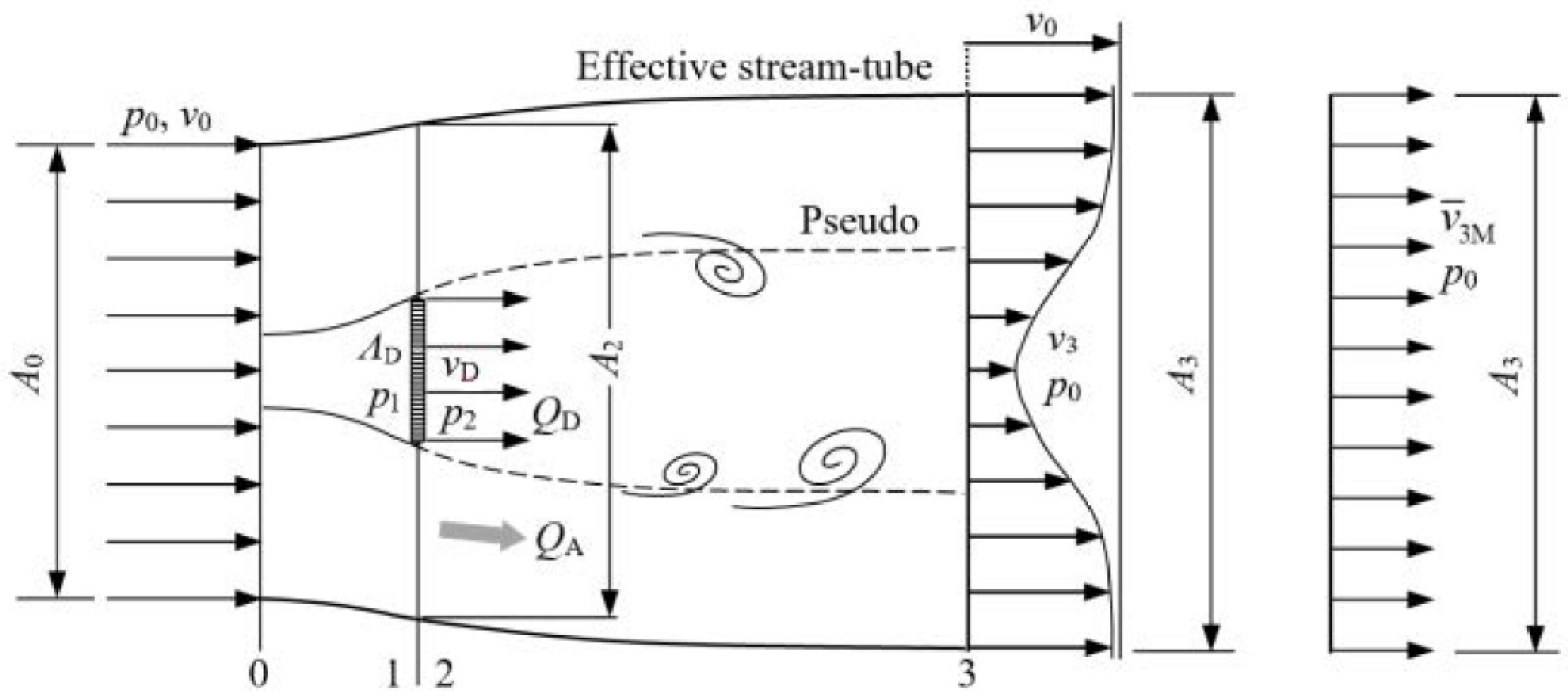
Figure 1, the control volume height (2
H) must be sufficiently large to contain the main part of the velocity deficit far behind the aerofoil, where the constant pressure,
p0, is restored. Then the thrust of the considered aerofoil is determined by the momentum equation alone:
Sufficient size of the control volume is required due to another fundamental fluid mechanical feature. The above momentum equation is established under the condition that the flow leaving the lateral surface of the control volume has an axial velocity component nearly equal to
v0. The flow on the control volume is thus almost parallel to the surface of the control volume. Since the
y-component of the velocity is negligible, the mass flow laterally leaving the control volume is also small. As can be seen from
Figure 1, this small value is only given by the small height
h, which is bounded by the corresponding stream-tube (shown by the flat solid line). It can be shown that the mean pressure along such a flat stream-tube is equal to
p0. Thus, the pressure within the small height
h can be assumed to be constant.
This feature of a sufficiently large control volume allows the control volume to be replaced by the corresponding stream-tube. This is simply because the volumetric flow rate () used in Equation (1) is actually the same volumetric flow rate through the stream-tube. In addition, because of the near constant pressure on the stream-tube, the axial components of all pressure forces on the entire stream-tube surfaces (inlet 2H0, side, and outlet 2H) must be completely compensated for. This is verified by Equation (1), in which the pressure force is not present.
The mean velocity
in the above equation is related to the momentum flux in the considered plane and is calculated as,
For a large control volume, the thrust from Equation (1) is independent of the size of the control volume. This can be verified by calculating
from Equation (1), given as,
with
v as the local flow velocity on the control volume, i.e., at
y =
H.
The calculated thrust in Equation (1) increases monotonically with the height of the control volume. Since the total thrust is a constant, the increase given in the above equation must tend to zero for a sufficiently large height (H) of the control volume. This is confirmed as the local velocity, v, gradually reaches the undisturbed velocity, v0. Here, the condition fully agrees with the condition for the application of Equation (1) that the axial velocity component vx at the side wall of the control volume (y = H) is almost equal to v0, as mentioned before. Other statements made in the context of Equation (1) are also validated, including the applicability of the corresponding flat stream-tube. The flow inside the control volume is thus almost unaffected by the flow outside and vice versa.
Appendix A also shows that for large stream-tubes, the walls of all flat stream-tubes are parallel, given by
.
Theoretically, extending the control volume to infinity, say
H→∞ and hence
A→∞, gives
, as directly obtained from Equation (2) with
(mean value theorem for integrals). Accordingly, one obtains the same for volumetric (
) and energy (
) flows as follows in completeness:
For the definition of and its application, see Equations (5) and (7) below.
The associated power loss or rate of energy dissipation in the flow is simply calculated as .
In practical applications, Equation (1) can be used to measure thrust by using a control volume of appropriate finite size without having to satisfy Equation (4). The background of such a measurement concept can be clarified. By approximating the velocity distribution,
v0–
v, to be comparable with the Gaussian function (
Appendix B for the case of an actuator disc), the main part of the thrust can be captured using Equation (2) by setting the upper bound of the integration to be a finite value. The remaining part, corresponding to the complementary error function, is negligible.
The main part of the deficit velocity profile is thus defined within the height
H, at which
is fulfilled. The deficit velocity is then mainly confined to the flat stream-tube and can be replaced by the equivalent mean velocity (
) for the momentum flow, as also shown in
Figure 1. The mean velocities for mass and energy flows and thus the energy equation again remain unused.
Taking this concept into account, in contrast to Equation (4), there is generally,
The power loss in the flow is again calculated as , as in the case of H→∞.
The flow model used in
Figure 1 for the determination of the thrust of the aerofoil can also be applied to the flow model of an actuator disc. In particular, the effective control volume satisfying
along the control volume can be replaced by the equivalent
flat stream-tube. This is of great practical significance. Unfortunately, almost all calculations to date that consider the flow at an actuator disc have used an incorrect control volume or stream-tube, as shown in
Section 4 and
Section 5 below.
3. Actuator Disc Flow Model
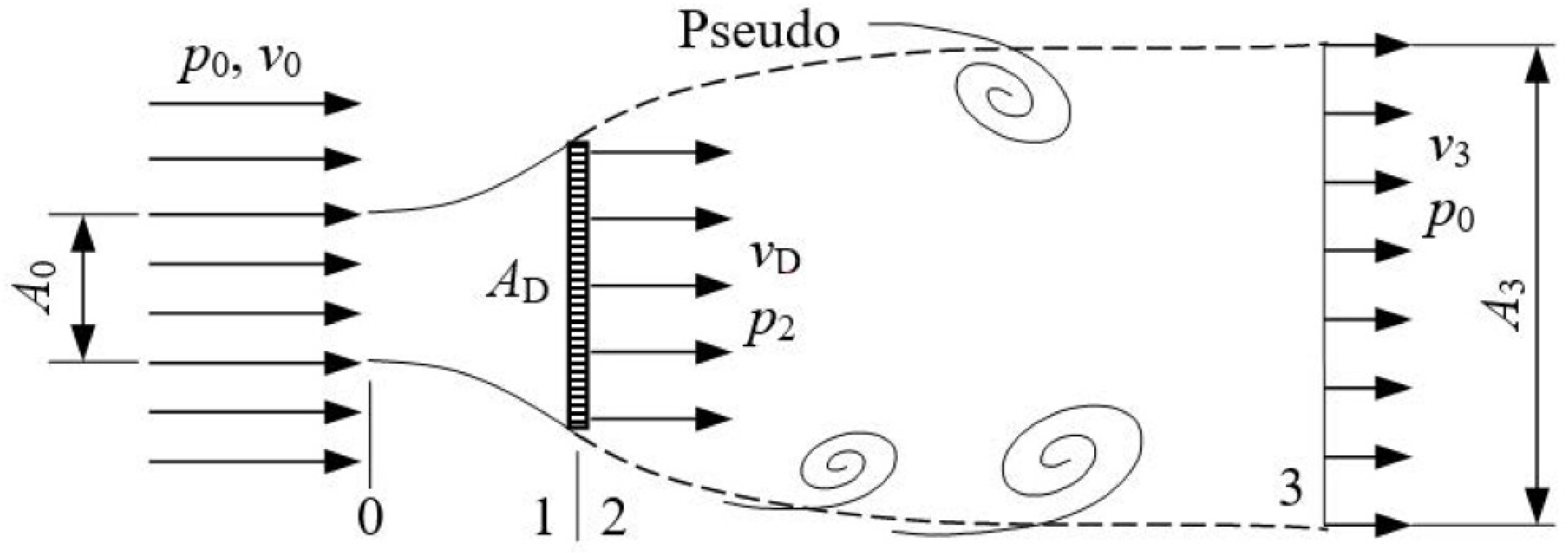
As stated in the introduction, the basic flow model for wind turbines is the flow through an actuator disc. Initially, according to
Figure 2, this was a flow model that only considers the pseudo stream-tube passing through the circumferential edge of the actuator disc. In almost all research works and textbooks (no references are given here), such a flow model was used as the basis of fluid mechanics for wind turbines. As will be shown in the following sections, the pseudo stream-tube is not valid as a useful control volume. The actuator disc itself can be regarded as a permeable disc at which the flow resistance and thus the volumetric flow rate can be changed. The effective stream-tube shown in
Figure 2 satisfies the condition of flatness (
Section 2) and can thus be used as a control volume to determine the thrust of the actuator disc.
The flow through the actuator disc is denoted by
, while the flow around the disc is given by
. The total volumetric flow rate in the control volume is
. As in
Section 2, the deficit velocity distribution in plane 3 is replaced by the equivalent mean velocity for the momentum flow, i.e.,
. Due to the finite size of the stream-tube considered, the condition given in Equation (5) applies.
The thrust of the actuator disc is then determined by the law of momentum applied to the mass flow rate
. According to Equation (1) this leads to,
The total power loss of the flow from plane 0 to plane 3 is obtained from the energy equation:
Here, the mean square velocity (integral term) represents the mean velocity for the energy flow in plane 3. Only if a sufficiently large control volume is used, the approximation
from Equation (4) is again applicable. Otherwise, there is generally
according to Equation (5) for the finite size of the control volume, which is often referred to as the practice of measurements. The case can be simulated. According to
Appendix B by assuming a Gaussian velocity profile in plane 3, the main part of the thrust (98%) could be obtained by a control volume of radius
R = 2
D with
D as the disc diameter. Within this control volume, the difference between the three mean velocities is also sufficiently small.
Based on fluid mechanics, the total power loss is again calculated as . As in Equation (3), a corresponding expression can also be found for the total power loss.
The total power loss between planes 0 and 3 is made up of two parts: one at the actuator disc in connection with
and another in the downstream flow because of the mixing of the two flows,
and
. Such a mixing of the flows and hence the associated energy dissipation is comparable with the Borda-Carnot shock loss, see
Section 6 below. The pseudo stream-tube in
Figure 2, therefore, does not exist. Accordingly, the equivalent mean velocity
within the area
A3 cannot be replaced by a mean velocity which is only restricted within the pseudo stream-tube.
Unfortunately, all significant fundamental calculations up to now have been based on the use of the control volume which is given by the pseudo stream-tube. At first glance, this is wrong because the mass transfer across the boundary into the pseudo stream-tube has been ignored. This clearly contradicts the fact that the volumetric flow rate at the outlet of the pseudo stream-tube is greater than at its inlet. Incidentally, as a control volume, the pseudo stream-tube behaves more similar to a diffuser than a flat stream-tube. As a result, the axial components of all pressure forces on the wall of the pseudo stream-tube, including the part from plane 0 to 1, do not vanish. They must be considered in addition to the thrust of the disc, as also shown in [
12] in terms of
FA and
FC. For further inconsistencies in the use of the pseudo stream-tube, see
Section 4 below.
Moreover, because the velocity, v, on the pseudo stream-tube is evidently smaller than v0, the condition from Equation (3), , is not fulfilled.
Based on the points of view presented above, as shown below in
Section 4, calculations leading to the Froude-Rankine theorem cannot be justified, even with the effective stream-tube control volume in
Figure 2. The main reason for this is the wrong connection between the total power loss and the thrust (other than
) and the disregard of the difference between the three mean velocities according to Equation (5). One will further see that Betz’s law, which is based on this theorem, is not justified either (
Section 5).
4. Unjustified Froude-Rankine Theorem
The actuator disc flow model was initiated by Froude after Rankine introduced the momentum theory. It is constructed to determine the thrust that depends on the flow through the actuator disc. As in all works dealing with the fundamentals of wind power using the actuator disc flow model, the pseudo stream-tube in
Figure 2 has always been taken as the control volume. Since the flow downstream of the disc is strongly subject to mixing with the surrounding flow and additional mass enters the control volume, none of mass, momentum, and energy balances can be established. The mass flow rate at the outlet of the pseudo stream-tube, for instance, is greater than that through the actuator disc. Accordingly, the condition for using Equation (1) for the momentum balance is no longer fulfilled. It is also not permissible to apply Bernoulli’s equation to the flow between plane 2 and plane 3. Otherwise, one would come to various contradictory conclusions.
First, by neglecting the flow mixing and mass transfer, the pseudo control volume would form a diffuser. If the energy law according to Bernoulli’s equation were applicable, then so would be the momentum law. This means that in addition to the thrust force on the disc, the pressure force on the diffuser wall (in the direction of flow) must also be taken into account. The same must be considered for the flow from plane 0 to plane 1. The total force obtained from the momentum equation would be their sum. Unfortunately, this diffuser effect has so far not been taken into account in all calculations of the flow in the pseudo stream-tube.
Second, in the special case of a negligible flow through the actuator disc () or at an impermeable circular disc (), there are and . Then it becomes impossible for the pressure to increase from at the disc to in plane 3. From Equation (1), one would also obtain , which is again mistaken.
Obviously, the use of the pseudo stream-tube results in great confusion in the calculations. The sad fact is that even the blade element momentum method (BEM) mentioned in the introduction is based on such a pseudo flow model.
The Froude-Rankine theorem was additionally initiated based on some other unfounded relations. To demonstrate all these points, as in
Section 2, we first consider the flat stream-tube as the effective control volume in the disc flow model according to
Figure 2. We will see that the Froude-Rankine theorem cannot be verified even in this case.
Following the derivation of the Froude-Rankine theorem, the thrust is calculated in the same law as Equation (6), but without specifying the type of mean velocity
used:
The total power loss caused by the disc within the stream-tube is calculated using the same mean velocity, as given by,
Except for the case of using a large control volume which leads to the conditions in Equation (4), different mean velocities should generally be used in Equations (8) and (9). We just ignore this minor disagreement with reality. Then, the two equations above are comparable with Equations (6) and (7) and can therefore be considered correct. The volume flow rate corresponds to the total flow rate in the effective stream-tube. The fact to be mentioned is that, as found throughout the literature, the above two equations are unfortunately always presented together with the flow through the pseudo stream-tube. For negligible flow rate through the actuator disc () there would be immediately which is obviously wrong.
The total power loss in the given form is actually composed of the partial loss at the actuator disc due to the flow through it () and the rate of energy dissipation in the downstream due to mixing of the two flows. The first part is simply given as , with vD as the flow velocity through the disc.
In deriving the Froude-Rankine theorem, the two equations given above are connected by the relationship
with
v2 as a velocity that is supposed to exist at the disc, i.e., in plane 2. Such a relation is physically unfounded because it does not agree with
according to
Section 2 and
Section 3. This is the crux of the subsequent unfounded derivation. On the one hand, the product
was simply considered as the power loss at the disc (plane 2). On the other hand, it is at the same time considered as the total power loss without taking into account the energy dissipation present in the flow downstream of the actuator disc.
Combining Equations (8) and (9) by
yields,
This is the so-called Froude-Rankine theorem. It is very confusing, as discussed below.
(1) The derivation of the theorem is based on the use of the same mean velocity (
) in Equations (8) and (9), which implies the fulfilment of Equation (4) and is thus only valid for a large control volume. Due to
, it then immediately follows
. This is the true feature of the Froude-Rankine theorem. Consequently, there is
that is fully consistent with the analyses performed in
Section 2 and
Section 3. This inference clearly indicates that the Froude-Rankine theorem is only applicable to the case of large stream-tubes at which
is fulfilled. It is unfounded for
which is given, for instance, in the consideration of the pseudo stream-tube.
(2) The Froude-Rankine theorem could not be derived if the respective mean velocities ( and ) in Equations (8) and (9) were used.
(3) The physical meaning of velocity
v2 is unclear. In contrast with hitherto assumed, the velocity itself does not represent a meaningful velocity in plane 2, neither around nor through the disc. The total power loss and the partial loss at the actuator disc are given by
and
, respectively, see
Section 6. Both have nothing to do with velocity
v2.
(4) In almost all research and applications in the field of wind energy, such as in the derivation of Betz’s law based on the use of the pseudo stream-tube control volume (see
Section 5 below), the product
has directly been taken as the volumetric flow rate through the actuator disc and even further used in Equations (8) and (9). This is confirmed as a further error. For an almost impermeable circular disc (
), e.g., as a special case there must be
v2 = 0 and
v3 = 0 at the same time. However, from Equation (10) this would never occur. For
v2 = 0 one would simply obtain
v3 = −
v0. This straightforwardly implies that the flow within the pseudo stream-tube does not satisfy the mass conservation. The related power loss would be erroneously
because of
T = 0 from Equation (8). Thus, using Equation (10) together with the pseudo stream-tube, all consequent results of further analyses, including Betz’s law, must be incorrect.
At this point, it would be helpful to better understand the problem by considering the flow through an orifice in a straight pipe, which is commonly used for flow measurement. If the flow velocity in the straight pipe is v0 and the drag force of the orifice is T, then the total power loss is given by . Here, the relevant velocity is the velocity in the straight pipe, not the one through the orifice. Neglecting the skin friction at the orifice, the power loss is completely caused by the redistribution of flow (mixing) in the pipe downstream of the orifice.
In some textbooks, the Froude-Rankine theorem is derived differently. One uses the pseudo stream-tube and applies the Bernoulli equation to the flows up- and downstream of the disc (
Figure 2), respectively. Both the up- and downstream flows are assumed to be lossless diffuser flows. Then, the pressure difference
and further the thrust
TD at the disc of area
AD is determined as,
This equation is equated with Equation (6) using the unfounded relationship . Then, Equation (10) is again obtained.
The problem with the calculation is the use of the unfounded expression . In Equation (6), actually represents the total volume flow rate through the effective stream-tube. Its expression in the term of makes no sense because velocity is physically meaningless: it is neither the velocity through the actuator disc nor the velocity in the flow around the disc. It is also not representative of an average velocity in the plane of the actuator disc.
For all these reasons, the Froude-Rankine theorem is obviously unjustified. It was even objected to by others at that time. According to the statement in [
11], engineer Lanchester, a pioneer in the actuator disc theory in the same era as Professor Froude also in the same British school, did not accept Froude’s result that the velocity through the disc is the average of the velocities far upstream and far downstream.
The incorrectness of Equation (10) was also indicated in [
12] with the conclusion that Betz’s law is not valid.
It should be mentioned that the Froude-Rankine theorem has also been applied to propellers and aircraft engines [
15,
16,
17]. There, from the point of view of the present paper, other serious inconsistencies in the theorem can be found.
A possible way to correctly calculate the actuator disc flow is to quantitatively calculate the energy dissipation that occurs in the downstream flow from plane 2 to plane 3. This is outlined in
Section 6.
5. Flaws in Betz’s Law
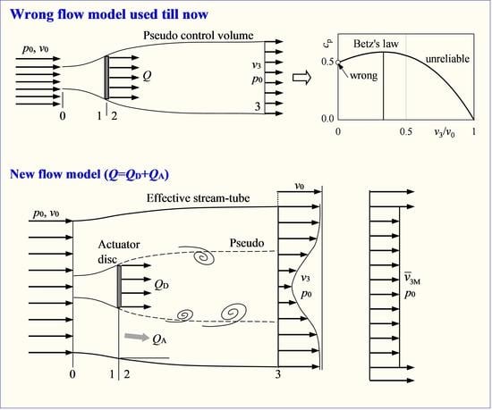
Betz’s law was initially derived using the Froude-Rankine theorem and the pseudo stream-tube flow model, as shown in
Figure 3. As stated in
Section 4, such a flow model is not valid, and the resultant Froude-Rankine theorem is not justified. For this reason, the use of the incorrect flow model and the unjustified Froude-Rankine theorem is recognized here as the
first flaw in the analyses leading to Betz’s law. It can be expected that various contradictory results will be given consequently. In a first step, Betz’s law and the related derivations should be presented based on
Figure 3.
The power loss caused by the actuator disc is calculated by Equation (9) without distinguishing the mean velocities for mass, momentum, and energy flows. For the volume flow, Betz used the unfounded relation with v2 from Equation (10). This is referred to as the second flaw in Betz’s law.
With the unfounded relation
, one obtains from Equation (9),
For simplicity, velocity notation is used instead of .
In wind turbine terminology, the power loss given in the above equation is considered to be the power extracted from the wind. It is not relevant here how this power extraction can be realized. The consideration is restricted to a one-dimensional flow without rotation.
The power of the wind, which is found far upstream of the actuator disc (plane 0 in
Figure 3) and within a cross-sectional area equal to the disc area, is given by
. The power coefficient of the wind turbine, in place of the actuator disc, is defined by relating Equation (12) to
:
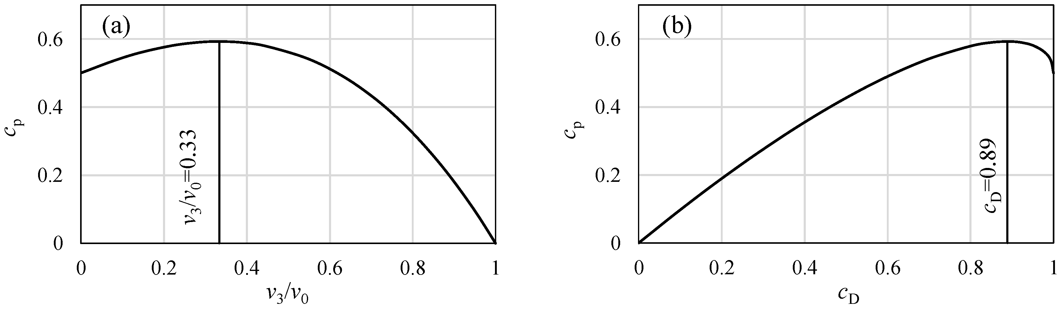
The power coefficient
is shown as a function of the velocity ratio
, as plotted in
Figure 4a. From the above equation, the maximum power coefficient at the velocity ratio
is obtainable. The maximum power coefficient itself is then calculated as,
This maximum is known as the Betz limit or Betz–Joukowsky limit, as mentioned in the introduction. Accordingly, Equation (13) and the condition are known as Betz’s law.
At an impermeable circular disc (
), we first suppose
. Then, the power coefficient from Equation (13) is
. This non-vanishing value is obviously incorrect. However, it has remained unexplained for the past century. Such an absurd result is clearly related to the absurd result of
given by Equation (10) for
. The mass conservation through the pseudo stream-tube (
Figure 3) would thus not be given.
To demonstrate further contradictions in connection with Betz’s law, Equation (10) is rewritten in the following form with respect to the pseudo volumetric flow rate
and
This equation, which has a pseudo character, signifies that the closed state of the actuator disc (
and therefore
) could not be included in the analyses. We already confirmed the related absurd result
from Equation (13). On the other hand, with
from the above equation and
, it follows from Equation (13),
A paradox in Equation (13) and
Figure 4a is confirmed this time by obtaining
in the closed disc case (
). This paradox has not yet been seen in the literature. This is because Equation (15) has hardly been used to check calculations. Sometimes, Betz’s law has even been derived via an axial induction factor
a which is defined by the relation
. In all these cases, the paradox is indeed hidden.
Further checks on mistaken Betz’s law can be made in view of the thrust coefficient of the actuator disc.
The thrust of an actuator disc is calculated using the thrust coefficient (
) as follows:
Equating this equation with Equation (6) with respect to
and
yields,
Similar to Equation (6), this equation basically applies to the flow model in
Figure 1, where the flow area
never becomes zero. It thus evidently indicates that the flow model in
Figure 3 is wrong because one would acquire a wrong result
for
in the case of an impermeable circular disc.
Multiplying both sides of Equation (15) by
A0 and then substituting
into Equation (18) yields,
Then, Equation (13) is also written as,
The power coefficient is now shown as a function of the thrust coefficient, as plotted in
Figure 4b. From this equation, the maximum power coefficient is found at
. The same maximum
cp is obtained as from Equation (14).
The fact to be mentioned is that the diagram of
Figure 4b was already found by Joukowsky, as reviewed in [
18]. The same application can also be found in [
3,
19]. Compared to
Figure 4a, the plot in
Figure 4b seems to be more meaningful, as the thrust coefficient
is a meaningful physical quantity and is directly related to the actuator disc used.
In the above calculations, another paradox is confirmed. From Equation (19), the thrust coefficient is obtained as
at the closed state of the actuator disc (
,
A0→0). From Equation (18), however, one obtains
. In addition, the case of
in
Figure 4a does not undoubtedly represent the closed state of the actuator disc, because Equation (10) simply gives
. Thus,
Figure 4a,b are inconsistent. The obvious reason for this discrepancy is that the condition of closed state of the disc does not apply. The true and decisive reason is the use of the incorrect flow model in
Figure 3 and the unfounded use of velocity
v2 in
.
We further consider the special case of the closed state of the actuator disc (impermeable), at which is obtained. Then Equation (19) also seems to be approximately consistent with the experiments. The thrust coefficient of a circular disc, as from measurements, takes a value in range . One could say that the discrepancy between the value and the measurements would be originated by the approximation to the theory, for instance, by neglecting the viscous effect. Then one would have a big problem if instead of the circular disc a rectangular plate of width b and infinite length is considered. The fact to be noted is that all the above calculations also apply to such an actuator plate. According to measurements, an impermeable rectangular plate of infinite length has a thrust coefficient . This value is in complete contradiction with Equations (19) and (20), not only in the closed state (), but also within the opening variation with . This circumstance demonstrates once again that the basic flow model used for Betz’s law is wrong.
Since the flow model used in
Figure 3 does not apply to the closed state of the actuator disc or plate, Betz’s maximum from Equation (14), which is found very close to the case of
(
Figure 4b), would not be convincing either. Looking further at the pressure difference over the actuator disc, another contradiction can be found. For all these reasons, Betz’s law cannot even be considered an approximation.
6. Possible Solution
Taking into account the flow model in
Figure 2 and using the stream-tube as the control volume, the volumetric flow rate is designated as
. It is composed of the flow through the actuator disc (
) and the flow around the disc (
). The flow between plane 0 and plane 1 is free of loss. The thrust exerted on the disc is determined by the pressure difference
with
between planes 1 and 2. For simplicity, uniform pressure distributions can be assumed. The associated power loss is then calculated as
with
vD as the flow velocity through the disc (
). It is a real velocity and has nothing in common with Equation (10) which has been confirmed to be unjustified. At the closed state of the disc, there is simply
and hence
. The flow between plane 2 and plane 3 is considered, contrary to all assumptions up to now, to be subject to energy dissipation, which arises from the mixing of two flows (
and
) and thus from the formation of vortices.
In fact, the mixing loss mentioned can be determined by knowing the two volume flows ( and ) within the effective stream-tube. This is exactly comparable with the calculation of the Borda-Carnot shock loss that occurs in the pipe when the flow suddenly expands. The difference is that here we are dealing with the mixing of two flows rather than the flow expansion in the pipe. The mechanism of flow redistribution, however, is the same. As for the calculation of Borda-Carnot shock loss, one must apply both the momentum and energy equations between plane 2 and plane 3. To this end, the flow around the disc can be assumed to be uniform for the total pressure of the undisturbed flow.
The total power loss in the flow is calculated as
according to
Section 2. The partial loss at the disc is correspondingly
. With the shock loss,
P23, in the downstream flow between plane 2 and plane 3, the energy balance is given by,
Considering the momentum and energy equations, the shock loss can be calculated with data in plane 2 () and data in plane 3 (). Another relationship required for a closed solution is Equation (7) based on the energy law. While the mean velocity in plane 3 is used for the momentum equation, the mean velocity must be used for the energy equation.
Only if the control volume is chosen sufficiently large (A3→∞), Equation (4) becomes available.
A further condition concerning the degree of opening of the actuator disc must be introduced. The partial power loss at the disc is calculated by
, where the thrust and the velocity are related by the degree of opening of the actuator disc. This degree of opening can be represented by the thrust coefficient
cD, which varying between 0 and 1.1. When using an actuator plate, the closed state is given by
cD = 2. Then, the thrust of the disc can be calculated directly from Equation (17). The remaining calculation should focus on the determination of the volumetric flow rate through the disc as a function of the thrust coefficient:
. Once this has been calculated, the power coefficient of the actuator disc viz. wind turbine can be calculated, analogous to Equation (13) or Equation (20), as a function of the thrust coefficient:
In deriving the Froude-Rankine theorem in
Section 4, the unfounded relationship
was used, which obviously does not represent the power loss at the disc. Its baseless use in Betz’s law has therefore led to diverse contradictions and paradoxes.
Contrary to Equation (20) and
Figure 4b, a vanishing power coefficient (
cp = 0) is obtained at the closed state of the actuator disc because of
. When the actuator disc is fully open, there is automatically
cp = 0 because of
.
The energy balancing by considering the energy dissipation in a similar way as for the Borda-Carnot shock loss provides an additional relation for a closed solution of the flow through an actuator disc. Thus, the statement “there is no unique prediction of a maximum value”, which is given in [
12] based on the use of the pseudo stream-tube, is no longer valid.
The main and most significant point of the calculation concept presented above is the calculation of the shock loss in the flow between plane 2 and plane 3. Since this requires further and detailed analyses, it cannot yet be shown in the present paper.
7. Summary
The actuator disc theory, the Froude-Rankine theorem, and Betz’s law have been the fundamentals of wind power technology. The associated fluid dynamics are reviewed using the momentum and energy laws. For the determination of the thrust of the actuator disc, the precondition of using the momentum equation is represented in terms of the applicability of the control volume. It has been concluded that the pseudo stream-tube is not applicable. The valid effective stream-tube is characterised by its flat shape.
The Froude-Rankine theorem has been shown to be unjustified. First, the momentum and energy equations cannot be applied to the flow in the pseudo stream-tube. Second, the total power loss and the thrust of the actuator disc are connected in the wrong way, i.e., by the unfounded velocity v2, which has no physical meaning and does not refer to the actuator disc either. Third, the Froude-Rankine theorem according to Equation (10) with does not work. It would be true and can be represented as only if applied to the large size stream-tube (flat shape).
Then two flaws in Betz’s law were pointed out. The first is related to the use of the wrong disc flow model regarding the pseudo stream-tube and the wrong Froude-Rankine theorem. The second flaw refers to the unfounded use of velocity from the Froude-Rankine theorem by considering as the volumetric flow rate through the actuator disc. Due to these two flaws, diverse contradictions and paradoxes have arisen in the calculations, which are particularly obvious in the case of a closed actuator disc or a rectangular plate (). Since the maximum power coefficient according to Betz’s law seems to occur near the closed state of the actuator disc, Betz’s limit of cp = 0.59 is highly questionable. For all these reasons, Betz’s law cannot be considered an approximation. It is simply wrong.
The possible solution for actuator disc flow was presented. It is based on the separate treatment of partial power losses that occur both at the actuator disc and in the downstream flow. The latter is caused by mixing and redistribution of the flows. It is comparable with the Borda-Carnot shock loss in a pipe flow with sudden expansion. The significant calculation algorithm has been outlined. It is intended to make the first step for scientists and engineers to work on improving and extending the associated theory. For this purpose, the basic relationship between the wind speed (v0), the velocity through the actuator disc (vD), the draft coefficient of the actuator disc (cD), and the power coefficient (cp) was established. By conducting extended studies, this relationship could at least be solved numerically.
Obviously, new fundamentals in the field of wind energy have to be worked out systematically. The fact is given here: In more than ten of the most available textbooks dealing with wind power and its applications, Betz’s law is presented all in the same manner. No remarks about the errors in the law are to be found there.
Extended studies should also include the transfer of proven turbine theories (e.g., Euler equation) from hydropower to wind power in order to improve the wind turbine design and operation optimisation. As this is not yet far progressed, the author want to propose his first attempt [
9].


