
A Hybrid Short-Term Load Forecasting Model Based on a Multi-Trait-Driven Methodology and Secondary Decomposition


Abstract
:1. Introduction
- (1)
- Based on the multi-trait analysis of the short-term load data, an appropriate decomposition method was constructed to extract modes with different periodicity patterns or data traits;
- (2)
- By embedding the method of multiple periodicities recognition, the IMSTL model can effectively identify and extract the multi-period patterns of the data;
- (3)
- A suitable judgment criterion is proposed to determine whether the modes need to be further decomposed, thereby improving the performance of the hybrid model.
2. Material and Methodology
2.1. The Framework of the Proposed Model
2.2. Multi-Trait-Driven Data Decomposition
2.2.1. Data Trait Testing Technique
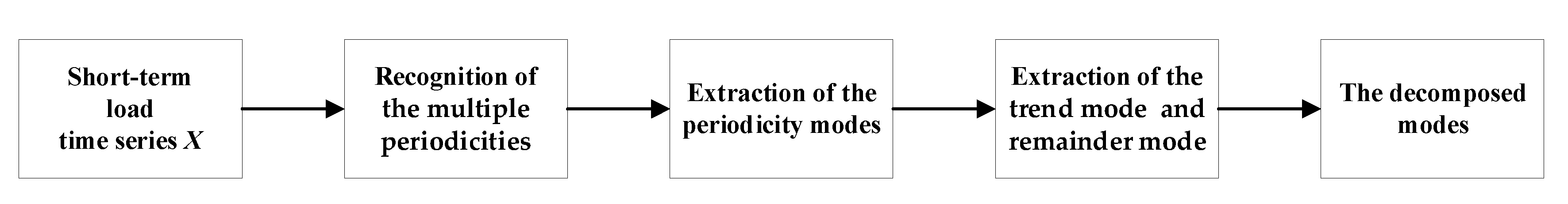
2.2.2. Decomposition Method
- (1)
- Based on the multi-period recognition procedure mentioned above, the length of each periodicity , (i = 1, …, M), can be determined and sorted in ascending order.
- (2)
- Decompose the time series data x(t) by STL to obtain their first periodicity mode with period length :where is the first periodicity mode, and is the corresponding residual.
- (3)
- Calculate the i-th periodicity mode and the i-th residual until all periodicity modes are extracted:
- (4)
- Smooth by loess to obtain the trend mode , and can be expressed as:where is the i-th periodicity mode, is the trend mode, and is the remainder mode.
2.3. Multi-Trait-Driven Secondary Decomposition
2.4. Multi-Trait-Driven Individual Prediction
2.5. Intermittency-Trait-Driven Ensemble Output
3. Results
3.1. Experimental Design
3.2. Experimental Results Analysis
3.2.1. Analysis of the Multi-Trait of the Short-Term Load Data
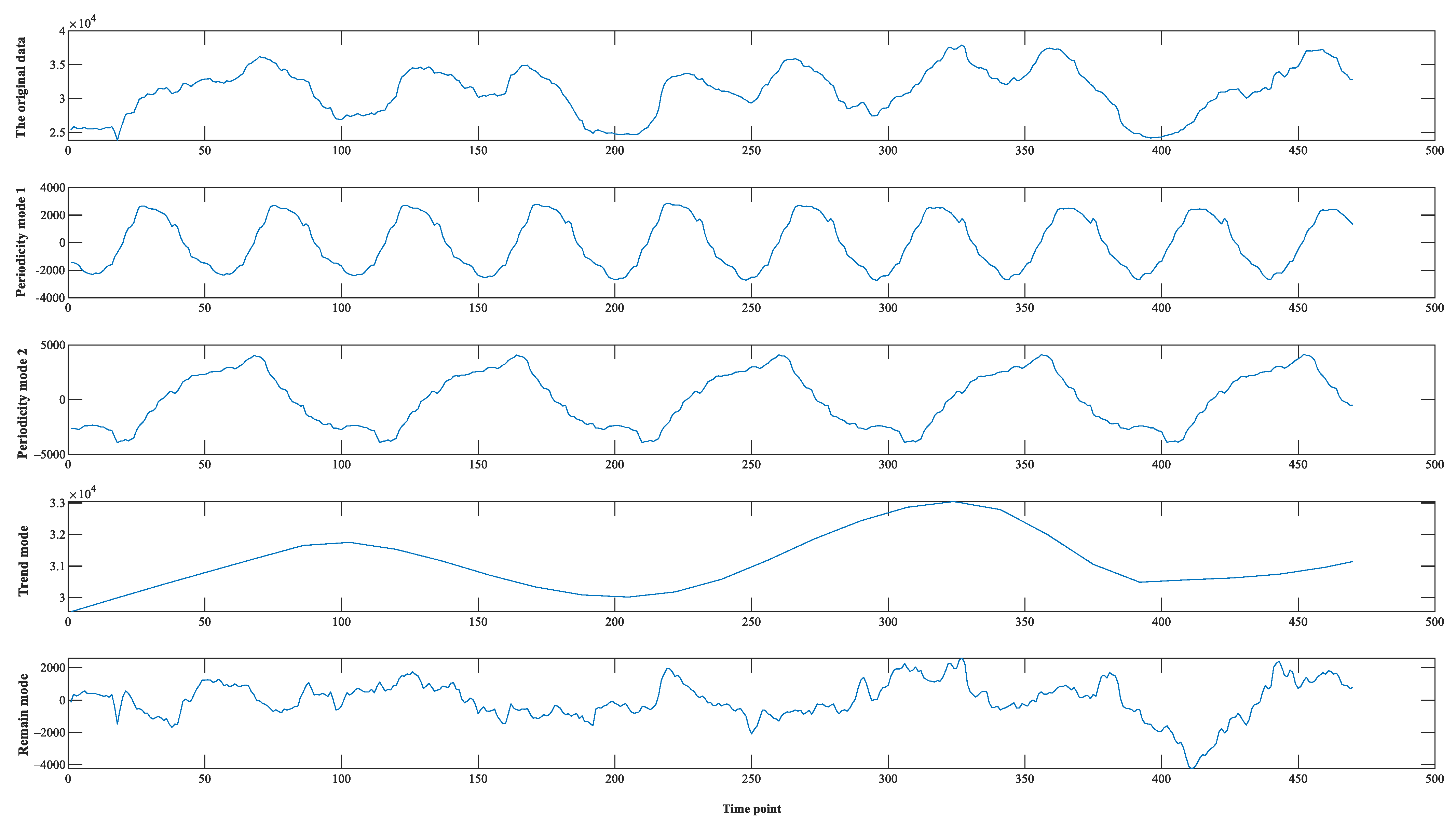
3.2.2. Data Decomposition Analysis
3.2.3. Multi-Trait-Driven Prediction Model Selection
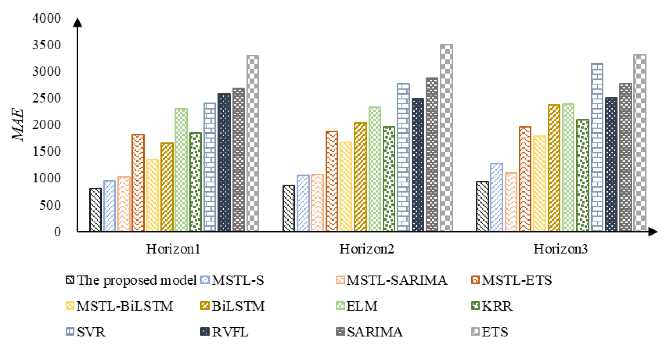
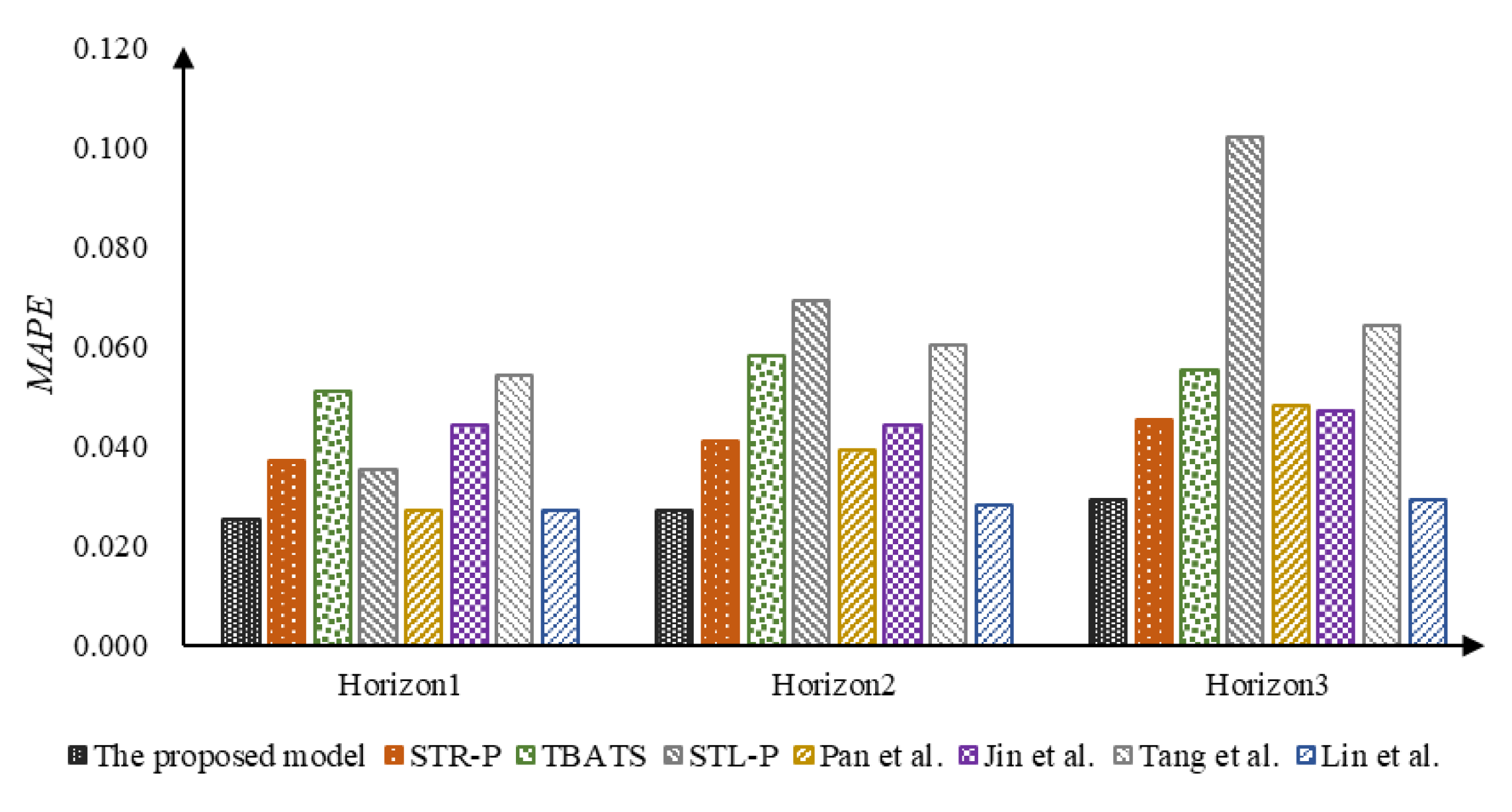
3.2.4. Comparison of Prediction Performance
4. Discussion
5. Conclusions
Author Contributions
Funding
Institutional Review Board Statement
Informed Consent Statement
Data Availability Statement
Conflicts of Interest
References
- Walser, T.; Sauer, A. Typical load profile-supported convolutional neural network for short-term load forecasting in the industrial sector. Energy AI 2021, 5, 100104. [Google Scholar] [CrossRef]
- Zhang, W.; Chen, Q.; Yan, J.; Zhang, S.; Xu, J. A novel asynchronous deep reinforcement learning model with adaptive early forecasting method and reward incentive mechanism for short-term load forecasting. Energy 2021, 236, 121492. [Google Scholar] [CrossRef]
- Liu, H.; Shi, J. Applying ARMA–GARCH approaches to forecasting short-term electricity prices. Energy Econ. 2013, 37, 152–166. [Google Scholar] [CrossRef]
- Chitalia, G.; Pipattanasomporn, M.; Garg, V.; Rahman, S. Robust short-term electrical load forecasting framework for commercial buildings using deep recurrent neural networks. Appl. Energy 2020, 278, 115410. [Google Scholar] [CrossRef]
- Dai, Y.; Zhao, P. A hybrid load forecasting model based on support vector machine with intelligent methods for feature selection and parameter optimization. Appl. Energy 2020, 279, 115332. [Google Scholar] [CrossRef]
- Wu, X.; Wang, Y.; Bai, Y.; Zhu, Z.; Xia, A. Online short-term load forecasting methods using hybrids of single multiplicative neuron model, particle swarm optimization variants and nonlinear filters. Energy Rep. 2021, 7, 683–692. [Google Scholar] [CrossRef]
- Massana, J.; Pous, C.; Burgas, L.; Melendez, J.; Colomer, J. Identifying services for short-term load forecasting using data driven models in a Smart City platform. Sustain. Cities Soc. 2017, 28, 108–117. [Google Scholar] [CrossRef]
- Rendon-Sanchez, F.; de Menezes, L.M. Structural combination of seasonal exponential smoothing forecasts applied to load forecasting. Eur. J. Oper. Res. 2019, 275, 916–924. [Google Scholar] [CrossRef]
- Kazemzadeh, M.-R.; Amjadian, A.; Amraee, T. A hybrid data mining driven algorithm for long term electric peak load and energy demand forecasting. Energy 2020, 204, 117948. [Google Scholar] [CrossRef]
- Dudek, G.; Pełka, P. Pattern similarity-based machine learning methods for mid-term load forecasting: A comparative study. Appl. Soft Comput. 2021, 104, 107223. [Google Scholar] [CrossRef]
- Kychkin, A.V.; Chasparis, G.C. Feature and model selection for day-ahead electricity-load forecasting in residential buildings. Energy Build. 2021, 249, 111200. [Google Scholar] [CrossRef]
- Cai, G.; Wang, W.; Lu, J. A novel hybrid short term load forecasting model considering the error of numerical weather prediction. Energies 2016, 9, 994. [Google Scholar] [CrossRef]
- Elamin, N.; Fukushige, M. Modeling and forecasting hourly electricity demand by SARIMAX with interactions. Energy 2018, 165, 257–268. [Google Scholar] [CrossRef]
- Li, C. A fuzzy theory-based machine learning method for workdays and weekends short-term load forecasting. Energy Build. 2021, 245, 111072. [Google Scholar] [CrossRef]
- Wang, Z.; Zhou, X.; Tian, H.; Huang, T. Hierarchical parameter optimization based support vector regression for power load forecasting. Sustain. Cities Soc. 2021, 71, 102937. [Google Scholar] [CrossRef]
- Hu, Y.; Qu, B.; Wang, J.; Liang, J.; Wang, Y.; Yu, K.; Li, Y.; Qiao, K. Short-term load forecasting using multimodal evolutionary algorithm and random vector functional link network based ensemble learning. Appl. Energy 2021, 285, 116415. [Google Scholar] [CrossRef]
- Khwaja, A.S.; Anpalagan, A.; Naeem, M.; Venkatesh, B. Joint bagged-boosted artificial neural networks: Using ensemble machine learning to improve short-term electricity load forecasting. Electric Power Syst. Res. 2020, 179, 106080. [Google Scholar] [CrossRef]
- Jiang, P.; Liu, F.; Song, Y. A hybrid forecasting model based on date-framework strategy and improved feature selection technology for short-term load forecasting. Energy 2017, 119, 694–709. [Google Scholar] [CrossRef]
- Zang, H.; Xu, R.; Cheng, L.; Ding, T.; Liu, L.; Wei, Z.; Sun, G. Residential load forecasting based on LSTM fusing self-attention mechanism with pooling. Energy 2021, 229, 120682. [Google Scholar] [CrossRef]
- Wang, S.; Wang, X.; Wang, S.; Wang, D. Bi-directional long short-term memory method based on attention mechanism and rolling update for short-term load forecasting. Int. J. Electr. Power Energy Syst. 2019, 109, 470–479. [Google Scholar] [CrossRef]
- Zhu, K.; Geng, J.; Wang, K. A hybrid prediction model based on pattern sequence-based matching method and extreme gradient boosting for holiday load forecasting. Electr. Power Syst. Res. 2021, 190, 106841. [Google Scholar] [CrossRef]
- Zhang, Z.; Hong, W.-C. Application of variational mode decomposition and chaotic grey wolf optimizer with support vector regression for forecasting electric loads. Knowl.-Based Syst. 2021, 228, 107297. [Google Scholar] [CrossRef]
- Yang, D.; Guo, J.E.; Sun, S.; Han, J.; Wang, S. An interval decomposition-ensemble approach with data-characteristic-driven reconstruction for short-term load forecasting. Appl. Energy 2022, 306, 117992. [Google Scholar] [CrossRef]
- Mohan, N.; Soman, K.P.; Sachin Kumar, S. A data-driven strategy for short-term electric load forecasting using dynamic mode decomposition model. Appl. Energy 2018, 232, 229–244. [Google Scholar] [CrossRef]
- Pan, D.; Xu, B.; Jun, M.A.; Ding, Q.; Quan, D.I.; Jinjin, Z.H.; Qian, Z. Short-term load forecasting based on EEMD-approximate Entropy and ELM. In Proceedings of the 2019 IEEE Sustainable Power and Energy Conference (iSPEC) 2019, Beijing, China, 21–23 November 2019; pp. 1772–1775. [Google Scholar] [CrossRef]
- Memarzadeh, G.; Keynia, F. Short-term electricity load and price forecasting by a new optimal LSTM-NN based prediction algorithm. Electr. Power Syst. Res. 2021, 192, 106995. [Google Scholar] [CrossRef]
- Tang, J.; Zhao, J.; Zou, H.; Ma, G.; Wu, J.; Jiang, X.; Zhang, H. Bus load forecasting method of power system based on VMD and Bi-LSTM. Sustainability 2021, 13, 10526. [Google Scholar] [CrossRef]
- Lin, Y.; Luo, H.; Wang, D.; Guo, H.; Zhu, K. An ensemble model based on machine learning methods and data preprocessing for short-term electric load forecasting. Energies 2017, 10, 1186. [Google Scholar] [CrossRef]
- Zhang, Z.; Hong, W.-C. Electric load forecasting by complete ensemble empirical mode decomposition adaptive noise and support vector regression with quantum-based dragonfly algorithm. Nonlinear Dyn. 2019, 98, 1107–1136. [Google Scholar] [CrossRef]
- Alipour, M.; Aghaei, H.; Norouzi, M.; Niknam, T.; Hashemi, S.; Lehtonen, M. A novel electrical net-load forecasting model based on deep neural networks and wavelet transform integration. Energy 2020, 205, 118106. [Google Scholar] [CrossRef]
- Singh, S.N.; Mohapatra, A. Data driven day-ahead electrical load forecasting through repeated wavelet transform assisted SVM model. Appl. Soft Comput. 2021, 111, 107730. [Google Scholar] [CrossRef]
- Yu, L.; Wang, Z.; Tang, L. A decomposition–ensemble model with data-characteristic-driven reconstruction for crude oil price forecasting. Appl. Energy 2015, 156, 251–267. [Google Scholar] [CrossRef]
- Yu, L.; Ma, M. A memory-trait-driven decomposition–reconstruction–ensemble learning paradigm for oil price forecasting. Appl. Soft Comput. 2021, 111, 107699. [Google Scholar] [CrossRef]
- Shah, I.; Iftikhar, H.; Ali, S.; Wang, D. Short-Term Electricity Demand Forecasting Using Components Estimation Technique. Energies 2019, 12, 2532. [Google Scholar] [CrossRef]
- Wu, Z.; Xia, X.; Xiao, L.; Liu, Y. Combined model with secondary decomposition-model selection and sample selection for multi-step wind power forecasting. Appl. Energy 2020, 261, 114345. [Google Scholar] [CrossRef]
- Xiang, L.; Li, J.; Hu, A.; Zhang, Y. Deterministic and probabilistic multi-step forecasting for short-term wind speed based on secondary decomposition and a deep learning method. Energy Convers. Manag. 2020, 220, 113098. [Google Scholar] [CrossRef]
- Emeksiz, C.; Tan, M. Multi-step wind speed forecasting and Hurst analysis using novel hybrid secondary decomposition approach. Energy 2022, 238, 121764. [Google Scholar] [CrossRef]
- Proietti, T.; Pedregal, D.J. Seasonality in high frequency time series. Econ. Stat. 2022. [Google Scholar] [CrossRef]
- Liu, X.; Iftikhar, N.; Huo, H.; Li, R.; Nielsen, P.S. Two approaches for synthesizing scalable residential energy consumption data. Future Gener. Comput. Syst. 2019, 95, 586–600. [Google Scholar] [CrossRef]
- Bouktif, S.; Fiaz, A.; Ouni, A.; Serhani, M.A. Single and multi-sequence deep learning models for short and medium term electric load forecasting. Energies 2019, 12, 149. [Google Scholar] [CrossRef]
- Tang, L.; Yu, L.; Liu, F.; Xu, W. An integrated data characteristic testing scheme for complex time series data exploration. Int. J. Inf. Technol. Decis. Mak. 2013, 12, 491–521. [Google Scholar] [CrossRef]
- Lopez, J.H. The power of the ADF test. Econ. Lett. 1997, 57, 5–10. [Google Scholar] [CrossRef]
- Tang, L.; Lv, H.; Yang, F.; Yu, L. Complexity testing techniques for time series data: A comprehensive literature review. Chaos Solitons Fractals 2015, 81, 117–135. [Google Scholar] [CrossRef]
- Unsworth, C.P.; Cowper, M.R.; McLaughlin, S.; Mulgrew, B. A new method to detect nonlinearity in a time-series: Synthesizing surrogate data using a Kolmogorov–Smirnoff tested, hidden Markov model. Phys. D Nonlinear Phenom. 2001, 155, 51–68. [Google Scholar] [CrossRef]
- Bartlett, M.S. Periodogram analysis and continuous spectra. Biometrika 1950, 37, 1–16. [Google Scholar] [CrossRef]
- Li, T. Detection and estimation of hidden periodicity in asymmetric noise by using quantile periodogram. In Proceedings of the 2012 IEEE International Conference on Acoustics, Speech and Signal Processing (ICASSP), Kyoto, Japan, 25–30 March 2012; pp. 3969–3972. [Google Scholar] [CrossRef]
- Daizadeh, I. Seasonal and secular periodicities identified in the dynamics of us FDA medical devices (1976–2020): Portends intrinsic industrial transformation and independence of certain crises. Ther. Innov. Regul. Sci. 2022, 56, 104–116. [Google Scholar] [CrossRef]
- Puech, T.; Boussard, M.; D’Amato, A.; Millerand, G. A fully automated periodicity detection in time series [A]. In International Workshop on Advanced Analysis and Learning on Temporal Data; Springer: Cham, Switzerland, 2020; pp. 43–54. [Google Scholar] [CrossRef]
- Cleveland, R.B.; Cleveland, W.S.; McRae, J.E. Terpenning I. STL: A seasonal-trend decomposition procedure based on loess. ournal of official statistics. J. Off. Stat. 1990, 6, 3–73. [Google Scholar]
- Bandara, K.; Hyndman, R.J.; Bergmeir, C. MSTL: A seasonal-trend decomposition algorithm for time series with multiple seasonal patterns. arXiv 2021, arXiv:2107.13462. [Google Scholar] [CrossRef]
- Yu, L.; Ma, Y.; Ma, Y.; Zhang, G. A complexity-trait-driven rolling decomposition-reconstruction-ensemble model for short-term wind power forecasting. Sustain. Energy Technol. Assess. 2022, 49, 101794. [Google Scholar] [CrossRef]
- Liu, X.; Zhang, Z.; Song, Z. A comparative study of the data-driven day-ahead hourly provincial load forecasting methods: From classical data mining to deep learning. Renew. Sustain. Energy Rev. 2020, 119, 109632. [Google Scholar] [CrossRef]
- Chahkoutahi, F.; Khashei, M. A seasonal direct optimal hybrid model of computational intelligence and soft computing techniques for electricity load forecasting. Energy 2017, 140, 988–1004. [Google Scholar] [CrossRef]
- Yu, L.; Ma, Y.; Ma, M. An effective rolling decomposition-ensemble model for gasoline consumption forecasting. Energy 2021, 222, 119869. [Google Scholar] [CrossRef]
- Dong, Y.; Ma, X.; Fu, T. Electrical load forecasting: A deep learning approach based on K-nearest neighbors. Appl. Soft Comput. 2021, 99, 106900. [Google Scholar] [CrossRef]
- Dokumentov, A.; Hyndman, R.J. STR: Seasonal-trend decomposition using regression. INFORMS J. Data Sci. 2021, 1–13. [Google Scholar] [CrossRef]
- De Livera, A.M.; Hyndman, R.J.; Snyder, R.D. Forecasting time series with complex seasonal patterns using exponential smoothing. J. Am. Stat. Assoc. 2011, 106, 1513–1527. [Google Scholar] [CrossRef]
- Jin, Y.; Guo, H.; Wang, J.; Song, A. A hybrid system based on LSTM for short-term power load forecasting. Energies 2020, 13, 6241. [Google Scholar] [CrossRef]


| Nature Trait | The Importance of Each Pattern Trait | |||||
|---|---|---|---|---|---|---|
| Nonstationarity | Nonlinearity | Complexity | Periodicity | Mutability | Randomicity | |
| The original data | × | √ | √ | 0.575 | 0.163 | 0.262 |
| Threshold-Based Filtering | Periodicity Test | Clustering | |
|---|---|---|---|
| Possible periods | [19.200, 32.000, 43.636, 48.000, 53.333, 68.571, 80.000, 96.000, 120.000, 160.000, 240.000, 480.000] | [43.636, 48.000, 53.333, 96.000] | [48.323, 96.000] |
| Nature Trait | The Importance of Each Pattern Trait | |||||
|---|---|---|---|---|---|---|
| Nonstationarity | Nonlinearity | Complexity | Periodicity | Mutability | Randomicity | |
| Periodicity mode 1 | √ | √ | × | 0.857 | - | 0.143 |
| Periodicity mode 2 | √ | √ | × | 0.932 | - | 0.068 |
| Trend mode | √ | √ | × | - | 0.337 | 0.663 |
| Remainder mode | √ | √ | √ | - | 0.096 | 0.904 |
| Mode | Model | F1 | F2 | F3 | F4 | F5 | ||||||||||
|---|---|---|---|---|---|---|---|---|---|---|---|---|---|---|---|---|
| MAPE | RMSE | MAE | MAPE | RMSE | MAE | MAPE | RMSE | MAE | MAPE | RMSE | MAE | MAPE | RMSE | MAE | ||
| Periodicity mode 1 | Bi-LSTM | 0.927 | 245.797 | 172.800 | 0.762 | 183.172 | 148.012 | 0.426 | 198.837 | 152.262 | 0.288 | 286.859 | 169.492 | 1.031 | 208.266 | 147.918 |
| ELM | 0.381 | 131.336 | 96.408 | 0.837 | 199.056 | 143.797 | 0.494 | 164.562 | 130.427 | 0.275 | 165.683 | 125.588 | 1.355 | 158.329 | 121.387 | |
| KRR | 1.100 | 248.675 | 178.268 | 0.570 | 267.152 | 198.993 | 0.231 | 219.067 | 159.969 | 0.267 | 223.608 | 158.665 | 1.400 | 194.533 | 142.468 | |
| SVR | 1.206 | 273.146 | 212.811 | 0.643 | 288.488 | 226.164 | 0.336 | 240.510 | 192.332 | 0.295 | 233.485 | 174.498 | 1.497 | 199.946 | 155.590 | |
| RVFL | 0.435 | 119.259 | 90.766 | 0.765 | 200.696 | 144.254 | 0.416 | 152.906 | 122.954 | 0.285 | 161.419 | 128.649 | 1.437 | 156.563 | 124.844 | |
| ES | 0.157 | 206.243 | 149.063 | 0.898 | 331.332 | 250.421 | 1.198 | 304.998 | 241.116 | 0.490 | 280.956 | 221.201 | 2.099 | 278.239 | 225.278 | |
| SARIMA | 0.217 | 206.993 | 155.856 | 0.226 | 171.155 | 105.006 | 0.048 | 46.834 | 35.228 | 0.049 | 50.458 | 39.188 | 0.034 | 29.947 | 21.969 | |
| Periodicity mode 2 | Bi-LSTM | 0.407 | 328.710 | 213.988 | 0.348 | 303.087 | 222.715 | 0.104 | 284.487 | 188.135 | 0.328 | 307.913 | 245.182 | 0.358 | 278.914 | 227.661 |
| ELM | 0.346 | 246.446 | 170.164 | 0.195 | 198.572 | 141.157 | 0.101 | 171.217 | 119.787 | 0.176 | 185.633 | 135.494 | 0.154 | 163.948 | 125.255 | |
| KRR | 0.477 | 269.428 | 184.659 | 0.285 | 282.065 | 210.790 | 0.136 | 220.858 | 151.651 | 0.237 | 238.050 | 175.000 | 0.210 | 224.272 | 163.845 | |
| SVR | 0.530 | 294.199 | 209.836 | 0.340 | 307.680 | 238.863 | 0.148 | 240.274 | 171.053 | 0.278 | 276.830 | 210.814 | 0.246 | 256.293 | 196.705 | |
| RVFL | 0.384 | 283.444 | 188.571 | 0.189 | 197.291 | 141.284 | 0.103 | 168.056 | 118.631 | 0.171 | 182.971 | 132.530 | 0.156 | 162.383 | 122.787 | |
| ES | 0.138 | 210.038 | 153.743 | 0.272 | 281.519 | 211.148 | 0.132 | 245.754 | 170.368 | 0.260 | 258.198 | 191.042 | 0.238 | 261.992 | 197.770 | |
| SARIMA | 0.173 | 216.284 | 153.938 | 0.070 | 157.681 | 73.852 | 0.004 | 7.010 | 5.479 | 0.006 | 5.966 | 4.875 | 0.006 | 6.499 | 4.946 | |
| Trend mode | Bi-LSTM | 0.003 | 95.910 | 79.191 | 0.001 | 24.979 | 21.014 | 0.006 | 307.894 | 211.088 | 0.005 | 179.874 | 153.440 | 0.001 | 29.363 | 16.417 |
| ELM | 0.003 | 2827.887 | 235.650 | 0.000 | 18.281 | 2.133 | 0.000 | 0.232 | 0.113 | 0.000 | 0.141 | 0.088 | 0.000 | 0.074 | 0.058 | |
| KRR | 0.001 | 66.677 | 66.139 | 0.001 | 74.555 | 73.408 | 0.001 | 51.457 | 50.941 | 0.001 | 69.497 | 69.406 | 0.001 | 66.456 | 66.385 | |
| SVR | 0.002 | 113.963 | 112.845 | 0.002 | 153.271 | 153.198 | 0.002 | 178.561 | 178.312 | 0.002 | 181.832 | 181.798 | 0.002 | 183.460 | 183.378 | |
| RVFL | 0.004 | 3524.889 | 291.528 | 0.000 | 44.607 | 5.317 | 0.000 | 0.244 | 0.116 | 0.000 | 0.142 | 0.079 | 0.000 | 0.076 | 0.058 | |
| ES | 0.001 | 19.060 | 17.462 | 0.000 | 2.661 | 0.590 | 0.001 | 32.204 | 31.108 | 0.001 | 38.091 | 34.116 | 0.000 | 9.852 | 8.427 | |
| ARIMA | 0.012 | 415.966 | 376.480 | 0.030 | 939.724 | 924.913 | 0.028 | 1043.801 | 873.919 | 0.034 | 1242.029 | 1056.441 | 0.014 | 464.305 | 427.642 | |
| Remainder mode | Bi-LSTM | 0.616 | 193.057 | 154.081 | 0.280 | 179.005 | 144.683 | 0.354 | 199.253 | 136.666 | 0.636 | 245.584 | 188.516 | 0.174 | 325.771 | 252.912 |
| ELM | 1.705 | 278.128 | 227.273 | 0.434 | 410.502 | 244.966 | 0.534 | 292.476 | 213.244 | 0.653 | 390.716 | 239.349 | 0.218 | 454.785 | 327.003 | |
| KRR | 1.893 | 251.111 | 200.934 | 0.356 | 249.167 | 181.776 | 0.508 | 253.489 | 199.368 | 0.578 | 277.362 | 186.589 | 0.202 | 347.059 | 266.996 | |
| SVR | 1.828 | 266.647 | 212.499 | 0.376 | 254.797 | 188.716 | 0.542 | 265.229 | 208.270 | 0.654 | 291.262 | 200.411 | 0.237 | 485.052 | 345.596 | |
| RVFL | 1.653 | 283.733 | 228.334 | 0.460 | 454.795 | 262.305 | 0.552 | 308.482 | 220.023 | 0.720 | 540.852 | 270.388 | 0.235 | 660.998 | 391.416 | |
| ES | 1.983 | 255.003 | 201.186 | 0.397 | 259.791 | 184.418 | 0.572 | 262.134 | 202.557 | 0.619 | 302.783 | 201.337 | 0.260 | 323.907 | 249.130 | |
| ARIMA | 2.215 | 246.489 | 190.728 | 0.480 | 247.095 | 182.575 | 0.815 | 240.575 | 189.495 | 0.709 | 272.573 | 182.989 | 0.320 | 292.273 | 221.723 | |
| SD-Bi-LSTM | 0.606 | 212.252 | 181.457 | 0.332 | 190.633 | 146.227 | 0.311 | 186.841 | 131.244 | 0.549 | 195.618 | 152.499 | 0.170 | 274.823 | 218.358 | |
| Mode | Model | |||
|---|---|---|---|---|
| MAPE | RMSE | MAE | ||
| Periodicity mode 1 | Bi-LSTM | 0.687 | 224.586 | 158.097 |
| ELM | 0.668 | 163.793 | 123.521 | |
| KRR | 0.714 | 230.607 | 167.673 | |
| SVR | 0.795 | 247.115 | 192.279 | |
| RVFL | 0.668 | 158.169 | 122.293 | |
| ES | 0.969 | 280.354 | 217.416 | |
| SARIMA | 0.115 | 101.078 | 71.449 | |
| Periodicity mode 2 | Bi-LSTM | 0.309 | 300.622 | 219.536 |
| ELM | 0.194 | 193.163 | 138.371 | |
| KRR | 0.269 | 246.935 | 177.189 | |
| SVR | 0.308 | 275.055 | 205.454 | |
| RVFL | 0.201 | 198.829 | 140.761 | |
| ES | 0.208 | 251.500 | 184.814 | |
| SARIMA | 0.050 | 77.495 | 47.643 | |
| Trend mode | Bi-LSTM | 0.003 | 127.604 | 96.230 |
| ELM | 0.001 | 569.323 | 47.608 | |
| KRR | 0.001 | 65.728 | 65.256 | |
| SVR | 0.002 | 162.217 | 161.906 | |
| RVFL | 0.001 | 713.992 | 59.420 | |
| ES | 0.001 | 19.845 | 17.693 | |
| ARIMA | 0.023 | 821.165 | 731.879 | |
| Remainder mode | Bi-LSTM | 0.412 | 228.534 | 175.372 |
| ELM | 0.709 | 365.321 | 250.367 | |
| KRR | 0.707 | 275.638 | 207.133 | |
| SVR | 0.727 | 312.597 | 231.098 | |
| RVFL | 0.724 | 449.772 | 274.493 | |
| ES | 0.766 | 280.723 | 207.726 | |
| ARIMA | 0.908 | 259.801 | 193.502 | |
| SD-Bi-LSTM | 0.394 | 212.033 | 165.957 | |
| Model | Horizon 1 | Horizon 2 | Horizon 3 | ||||||
|---|---|---|---|---|---|---|---|---|---|
| MAPE | RMSE | MAE | MAPE | RMSE | MAE | MAPE | RMSE | MAE | |
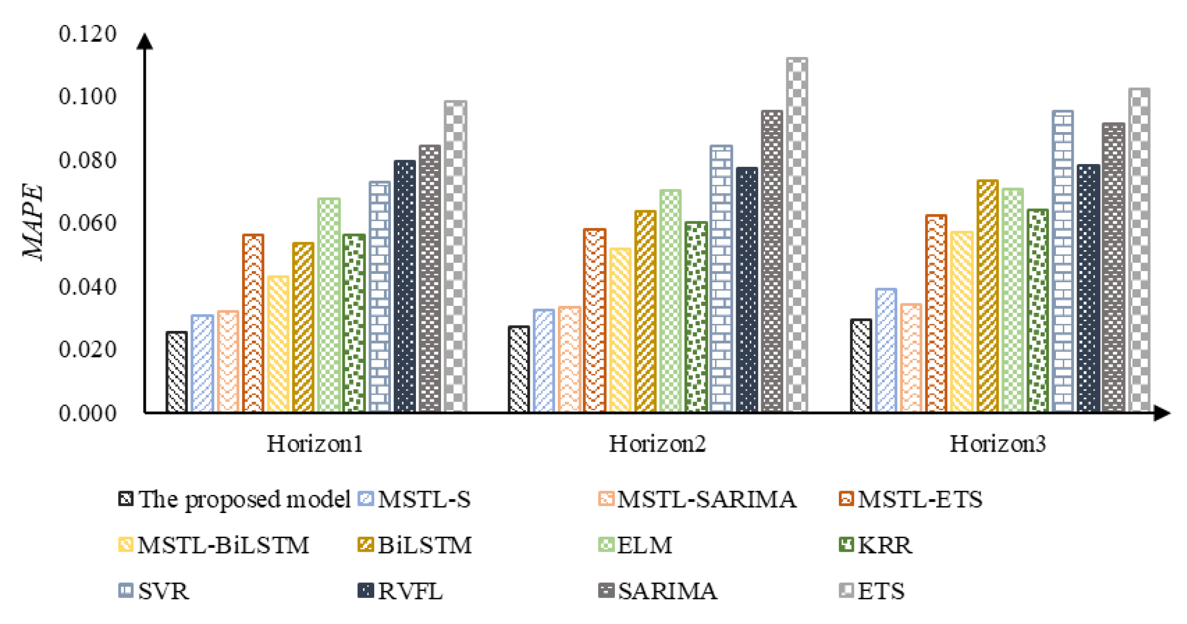
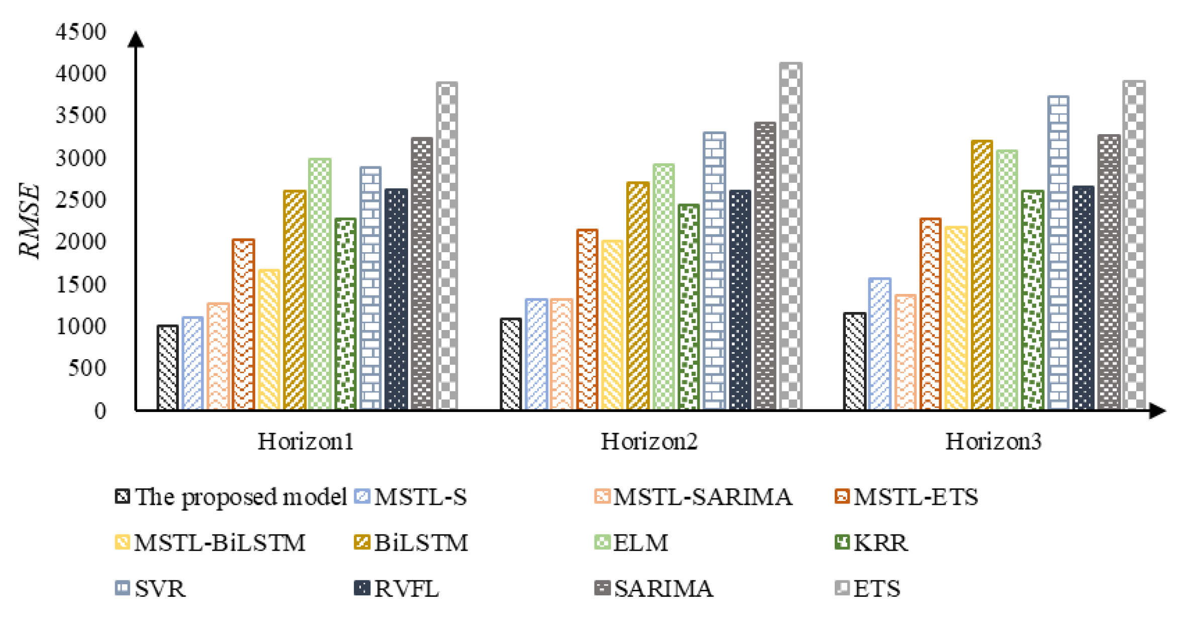
| The proposed model | 0.025 | 996.632 | 803.840 | 0.027 | 1075.094 | 863.915 | 0.029 | 1153.009 | 925.959 |
| IMSTL-S | 0.030 | 1097.379 | 945.976 | 0.032 | 1313.271 | 1053.374 | 0.039 | 1562.250 | 1273.193 |
| IMSTL-SARIMA | 0.032 | 1254.016 | 1014.147 | 0.033 | 1306.357 | 1057.062 | 0.034 | 1356.456 | 1098.243 |
| IMSTL-ES | 0.056 | 2026.460 | 1803.078 | 0.058 | 2141.056 | 1873.246 | 0.062 | 2273.182 | 1962.798 |
| IMSTL-Bi-LSTM | 0.043 | 1656.921 | 1340.371 | 0.052 | 2007.111 | 1661.422 | 0.057 | 2158.918 | 1775.344 |
| Bi-LSTM | 0.053 | 2591.693 | 1641.828 | 0.063 | 2688.045 | 2023.559 | 0.073 | 3191.726 | 2372.660 |
| ELM | 0.068 | 2981.484 | 2287.289 | 0.070 | 2901.366 | 2317.169 | 0.070 | 3077.101 | 2385.460 |
| KRR | 0.056 | 2261.984 | 1832.726 | 0.060 | 2427.685 | 1961.387 | 0.064 | 2589.605 | 2089.087 |
| SVR | 0.073 | 2868.298 | 2388.849 | 0.084 | 3291.700 | 2768.444 | 0.095 | 3719.329 | 3140.454 |
| RVFL | 0.079 | 2617.263 | 2569.141 | 0.077 | 2591.416 | 2484.866 | 0.078 | 2648.145 | 2501.780 |
| ES | 0.084 | 3218.942 | 2668.784 | 0.095 | 3394.825 | 2864.424 | 0.091 | 3251.437 | 2760.568 |
| SARIMA | 0.098 | 3888.001 | 3282.341 | 0.112 | 4119.156 | 3487.136 | 0.102 | 3897.657 | 3303.147 |
| Target Model | Benchmark Model | ||||||||||
|---|---|---|---|---|---|---|---|---|---|---|---|
| IMSTL-S | IMSTL-SARIMA | IMSTL-ES | IMSTL-Bi-LSTM | Bi-LSTM | ELM | KRR | SVR | RVFL | ES | SARIMA | |
| The proposed model | −2.335 (0.011) | −7.354 (0.000) | −12.242 (0.000) | −7.053 (0.000) | −2.772 (0.003) | −7.574 (0.000) | −8.744 (0.000) | −10.875 (0.000) | −28.268 (0.000) | −11.407 (0.000) | −10.598 (0.000) |
| IMSTL-S | −4.563 (0.000) | −10.739 (0.000) | −5.871 (0.000) | −2.654 (0.004) | −7.229 (0.000) | −7.724 (0.000) | −10.008 (0.000) | −26.213 (0.000) | −11.079 (0.000) | −9.911 (0.000) | |
| IMSTL-SARIMA | −8.909 (0.000) | −4.426 (0.000) | −2.475 (0.007) | −6.831 (0.000) | −6.871 (0.000) | −9.421 (0.000) | −21.491 (0.000) | −10.804 (0.000) | −9.527 (0.000) | ||
| IMSTL-ES | 3.723 (0.000) | −1.251 (0.106) | −4.344 (0.000) | −1.293 (0.098) | −5.065 (0.000) | −8.575 (0.000) | −8.631 (0.000) | −7.706 (0.000) | |||
| IMSTL-Bi-LSTM | −1.957 (0.026) | −6.746 (0.000) | −8.067 (0.000) | −10.901 (0.000) | −13.675 (0.000) | −12.173 (0.000) | −7.963 (0.000) | ||||
| Bi-LSTM | −0.955 (0.171) | 0.964 (0.167) | −0.292 (0.385) | −0.063 (0.474) | −3.785 (0.000) | −1.715 (0.044) | |||||
| ELM | 5.571 (0.000) | 2.391 (0.008) | 2.022 (0.022) | −6.739 (0.000) | −1.072 (0.142) | ||||||
| KRR | −11.882 (0.000) | −4.983 (0.000) | −12.223 (0.000) | −5.981 (0.001) | |||||||
| SVR | 0.815 (0.207) | −10.131 (0.000) | −3.084 (0.001) | ||||||||
| RVFL | −6.728 (0.000) | −3.957 (0.000) | |||||||||
| ES | 3.028 (0.001) | ||||||||||
| Model | Horizon 1 | Horizon 2 | Horizon 3 | ||||||
|---|---|---|---|---|---|---|---|---|---|
| MAPE | RMSE | MAE | MAPE | RMSE | MAE | MAPE | RMSE | MAE | |
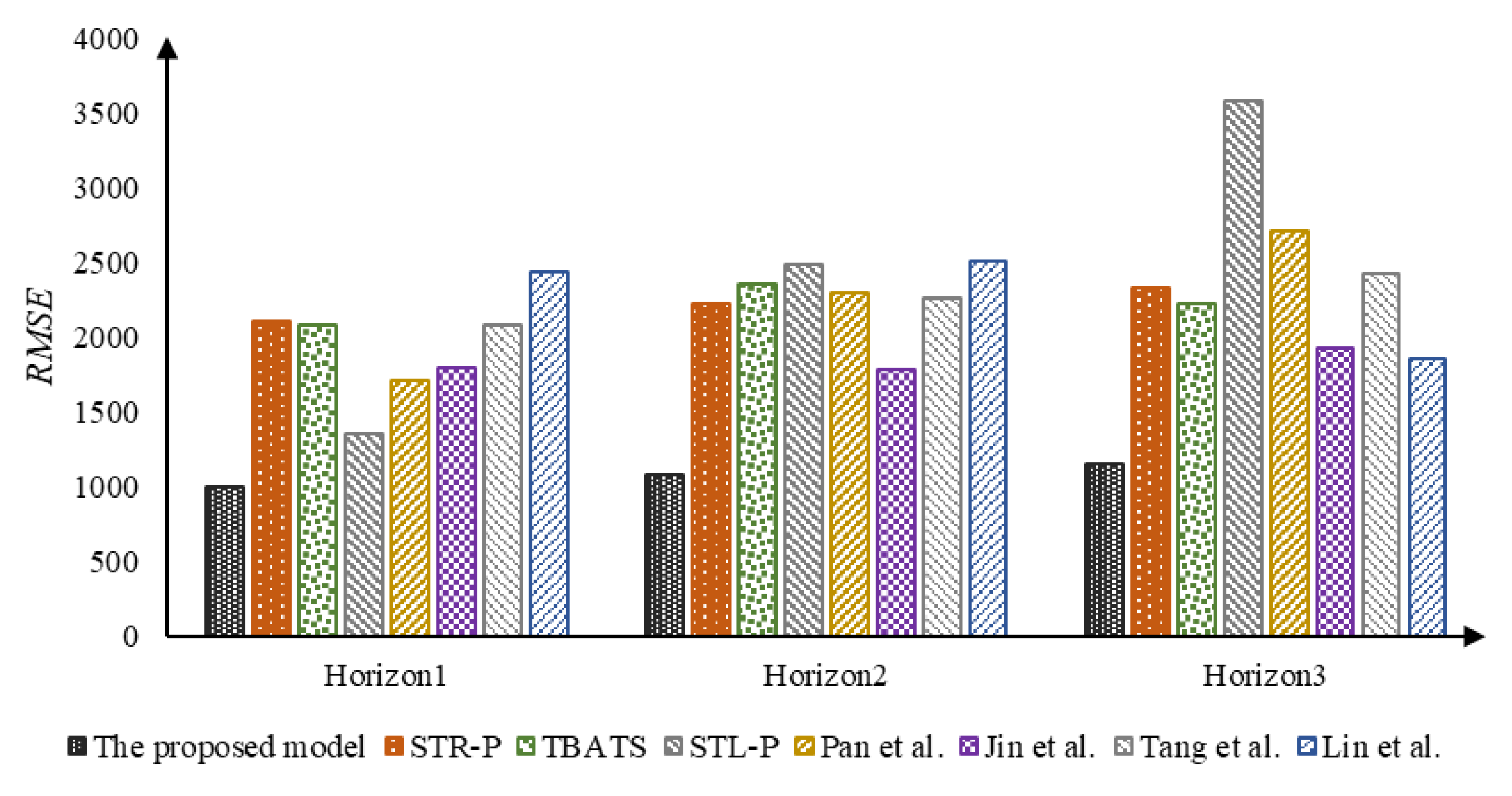
| The proposed model | 0.025 | 996.632 | 803.840 | 0.027 | 1075.094 | 863.915 | 0.029 | 1153.009 | 925.959 |
| STR-P | 0.030 | 1097.379 | 945.976 | 0.032 | 1313.271 | 1053.374 | 0.039 | 1562.250 | 1273.193 |
| TBATS | 0.032 | 1254.016 | 1014.147 | 0.033 | 1306.357 | 1057.062 | 0.034 | 1356.456 | 1098.243 |
| STL-P | 0.056 | 2026.460 | 1803.078 | 0.058 | 2141.056 | 1873.246 | 0.062 | 2273.182 | 1962.798 |
| Pan et al. [25] | 0.043 | 1656.921 | 1340.371 | 0.052 | 2007.111 | 1661.422 | 0.057 | 2158.918 | 1775.344 |
| Jin et al. [58] | 0.053 | 2591.693 | 1641.828 | 0.063 | 2688.045 | 2023.559 | 0.073 | 3191.726 | 2372.660 |
| Tang et al. [27] | 0.068 | 2981.484 | 2287.289 | 0.070 | 2901.366 | 2317.169 | 0.070 | 3077.101 | 2385.460 |
| Lin et al. [28] | 0.056 | 2261.984 | 1832.726 | 0.060 | 2427.685 | 1961.387 | 0.064 | 2589.605 | 2089.087 |
| Target Model | Benchmark Model | ||||||
|---|---|---|---|---|---|---|---|
| STL-P | STR-P | TBATS | Pan et al. [25] | Jin et al. [58] | Tang et al. [27] | Lin et al. [28] | |
| The proposed model | −4.419 (0.000) | −8.241 (0.000) | −6.293 (0.000) | −2.420 (0.008) | −6.761 (0.000) | −9.467 (0.000) | −1.668 (0.048) |
| STR-P | 0.116 (0.453) | 3.394 (0.000) | 1.313 (0.095) | 1.371 (0.086) | 0.101 (0.459) | −0.487 (0.313) | |
| TBATS | 6.018 (0.000) | 1.660 (0.049) | 4.266 (0.000) | −0.062 (0.475) | −0.541 (0.294) | ||
| STL-P | −1.339 (0.091) | −4.009 (0.000) | −6.805 (0.000) | −1.374 (0.085) | |||
| Pan et al. [25] | −0.373 (0.354) | −1.725 (0.043) | −0.987 (0.162) | ||||
| Jin et al. [58] | −5.657 (0.000) | −0.917 (0.179) | |||||
| Tang et al. [27] | −0.542 (0.294) | ||||||
Publisher’s Note: MDPI stays neutral with regard to jurisdictional claims in published maps and institutional affiliations. |
© 2022 by the authors. Licensee MDPI, Basel, Switzerland. This article is an open access article distributed under the terms and conditions of the Creative Commons Attribution (CC BY) license (https://creativecommons.org/licenses/by/4.0/).
Share and Cite
Ma, Y.; Yu, L.; Zhang, G. A Hybrid Short-Term Load Forecasting Model Based on a Multi-Trait-Driven Methodology and Secondary Decomposition. Energies 2022, 15, 5875. https://doi.org/10.3390/en15165875
Ma Y, Yu L, Zhang G. A Hybrid Short-Term Load Forecasting Model Based on a Multi-Trait-Driven Methodology and Secondary Decomposition. Energies. 2022; 15(16):5875. https://doi.org/10.3390/en15165875
Chicago/Turabian StyleMa, Yixiang, Lean Yu, and Guoxing Zhang. 2022. "A Hybrid Short-Term Load Forecasting Model Based on a Multi-Trait-Driven Methodology and Secondary Decomposition" Energies 15, no. 16: 5875. https://doi.org/10.3390/en15165875
APA StyleMa, Y., Yu, L., & Zhang, G. (2022). A Hybrid Short-Term Load Forecasting Model Based on a Multi-Trait-Driven Methodology and Secondary Decomposition. Energies, 15(16), 5875. https://doi.org/10.3390/en15165875