1. Introduction
The electrical system is undergoing a modernization process. The new ways of generating and consuming energy increasingly increase the complexity of its control and operation. The growing use of renewable sources such as wind and solar are examples of this process. These sources are characterized by not allowing control on demand, being intermittent and difficult to predict [
1]. The share of renewable energy sources in power generation shall reach up to 65% in 2050 [
2]. The system’s complexity grows in parallel with this process. In this context, information on the load side and predictions of its behavior are essential for the safety and stability of the system.
The ability to measure and interpret data in real-time at each consumer unit makes it possible to obtain new services such as estimating the daily consumption curve and controlling the load of each individual consumer. The smart meters are presented as the connection point for creating and distributing this information. Unlike conventional meters, data analysis, load management, and load forecasting can be achieved using smart meters [
3,
4]. This new information allows the consumer himself to contribute to more rational use of energy.
Thus, the individual short-term load forecasting (STLF) in smart meters gains importance as part of the progress towards a more interconnected system. Individual short-term load forecasting can help the demand side management, (DSM) [
1,
5] and the response demand (DR) [
6], which creates more stability in the system through indirect control of electricity consumption.
Improving load forecasting is the goal of several studies [
4,
5,
6,
7,
8,
9,
10,
11,
12,
13,
14,
15,
16,
17,
18]. However, studies on individual consumers are scarce. The reason for this is that the low or medium voltage load forecast has a high degree of randomness and dependence on the characteristics of each consumer, which reduces the accuracy of the forecasts.
The papers that perform STLF use different methodologies to reduce their errors. One of them is to aggregate the measurement of several smart meters, making the prediction of the aggregate load [
1,
7]. A second way found is to group measurements from consumers with similar behavior to train machine learning algorithms [
4,
6,
8]. With these methodologies it is possible to reduce the randomness of the database, however, it creates a dependency on the expected characteristic for the data and an infrastructure of meters is needed. Another proposed methodology consists of pre-processing the database, which can be done by treating the noise in the database [
9] or by selecting the best features for prediction through feature engineering [
10].
Treating the database and selecting the best features can significantly reduce the prediction error. Therefore, the present work aims to develop a methodology for short-term load forecasting in individual consumers. The methodology consists of using feature engineering and feature extraction techniques to select the most significant features from the database and, consequently, reduce the forecast error associated with the randomness of the measurements.
The main contributions of this paper can be summarized as follows:
Propose the use of the mutual information technique as one of the criteria to select the most important features for load forecasting;
Propose a methodology for choosing significant features based on the joint application of mutual information and correlation techniques;
Compare STLF results with different machine learning techniques;
Improved short-term load forecasting in individual consumers by pre-processing and feature selection.
Predictive models of electricity consumption will be developed in association with the main machine learning techniques found in the literature with application in short-term load forecasting.
The four machine learning techniques implemented are:
Support Vector Regression (SVR);
Feedforward Multilayer Perceptron (MLP);
Long short-term memory (LSTM);
ARTMAP-Fuzzy.
The forecasting models and the methodology for selecting the features are evaluated for error in tests performed with a database of an individual consumer smart meter belonging to the distribution system of Paraíba in Brazil.
The rest of this paper is organized as follows: in
Section 2 we review the relevant literature.
Section 3 describes our methodology for short-term load forecasting and
Section 4 presents the results of our tests on an actual load database. In
Section 5 we discuss our results and provide an outlook for future research.
2. Related Work
The energy consumption of a user is composed of the set of devices that demand electrical energy and that together create a consumption pattern represented by a load curve. Load forecasting can be performed from historical consumption data and other attributes that influence energy consumption. Many works use this data with machine learning techniques to predict the behavior pattern of consumers. In this section, some of the recent approaches related to STLF are briefly presented. The papers are summarized in
Table 1.
Kong et al. [
11] proposed the use of an LSTM neural network as a way of identifying the consumption pattern and making a 30-min load forecasting for a residential unit. They used a vast database with 3 months of consumption of 69 consumer units. The load curve of each residence is predicted individually. The results are compared with the state of art techniques, including the MLP neural network and the K-Nearest Neighbor (KNN) algorithm. The LSTM was considerably better than the others analyzed, with an absolute mean percentage error (
MAPE) of 44.06%, while the best result among the others analyzed was 49.49%.
Kong et al. [
12], in another paper, used a network of sensors spread over a residence, measuring the consumption of the main loads to help predict the total load. The LSTM neural network with a forecast horizon of 30 min is used. The work achieves a considerable reduction in forecast error when compared to its previous work. The results of the proposed model are compared with MLP and KNN networks. The LSTM network is considerably better than the others analyzed.
Alves [
13] used an ARTMAP-Fuzzy neural network for STLF for individual users. The maximum, minimum, and average values of energy consumption are extracted and used as input for the predictor model in addition to the time series of energy consumption and temporal variables. A considerable improvement in the prediction of energy consumption is observed when the new extracted attributes are used. The
MAPE of forecasts ranged from 17.06% to 38.09%.
Similar to [
12], Haq et al. [
14] performed the forecast of the daily demand peak of a residence from the measurement in its main loads. The authors carry out the consumption forecast of each load individually and consider the results as inputs for the forecast of the daily demand peak, obtaining a considerable reduction of the forecast error.
In Park et al. [
10], authors use the pre-processing of data with identification and correction of errors and the creation and selection of features to improve the result of the prediction model. Pearson’s correlation coefficient is used as a selection criterion for predictive features. Temporal and climatic variables and statistical data extracted from these time series are taken into account during the feature extraction process. The work used a sliding window in time to simulate an online forecast. As a result, the relationship between the prediction improvement and the computational cost with the window growth is observed.
Moon et al. [
15] carried out a similar work focused on load of a residential building. The authors study the optimal data window for carrying out the short-term load forecast and use Pearson’s coefficient as a criterion for identifying the most significant attributes. The proposed prediction technique is called COSMOS, based on the stacking ensemble of MLP neural networks. The authors also demonstrate the importance of optimizing the hyperparameters of the forecasting technique, which has a significant impact on the final error.
In Ayub et al. [
16] feature extraction and selection are used to improve short-term load forecasting. The authors propose the use of Random Forest and Extreme Gradient Boosting techniques to determine the importance of features. In addition, the RFE technique is used to determine the redundant features, removing the less important features for the forecast. As a result, the article achieves an accuracy of up to 96.33% in the STLF.
Roth et al. [
17] use a database of 120 smart meters of residential apartments in Singapore and forecast hourly consumption at the individual level. The apartments have smart meters in the main electrical equipment and these data are considered during the forecast. To prepare the database, an feature selection process is carried out using the Spike-and-Slab method presented in [
22], in which the most significant features for prediction are selected. As a result, an improvement in the forecast is observed with the use of features related to measurements in the main loads of the residence, mainly with larger forecast horizons.
In Jung et al. [
18] the STLF model is proposed using attention-based GRU neural network to give more weight to the features with more relevance for forecasting. Through tests carried out with data from real consumers, an improvement in the prediction is proven when compared to state-of-the-art techniques.
As demonstrated above, many works use interactive techniques to perform the STLF, as is the case with [
15,
16]. Due to the characteristics of these methods, they are associated with long training times and their results are difficult to interpret. Alternatively, the author of [
23] describes a new topology and training algorithm for a non-interactive neural structure. The approach is based on a Successive Geometric Transformations Model (SGTM) neural link. With the new topology, advantages such as faster training, data pre-processing, selection of the most significant attributes, and flexibility in solving different types of tasks are achieved. Some authors have applied the topology to prediction tasks [
19] or for optimized identification of regression coefficients [
20], demonstrating the feasibility of the technique.
Prakash and Sydulu [
21] develop a similar methodology with the aim of performing the STLF in a non-interactive way. For this, a state estimation approach is used to determine the ideal set of weights of neurons in a neural network. The methodology is applied to real load data in a power distribution system. As a result, STLF is achieved with an error like a common neural network, but with a drastic reduction in training time.
As can be confirmed by the review presented, the challenges encountered in load forecasting of individual users are still present and are the motivation for the most recent work in the STLF. To improve load forecasting, some works make use of measurement at several points as in [
12,
14,
17]. These works have the problem of needing a structure of meters spread throughout the residence. Other works like [
15,
16,
21,
23] use pre-processing and feature selection techniques to improve load forecasting. These works demonstrate that the correct selection and treatment of data is capable of significantly reducing the forecast error.
In this paper, the author develops a system for STLF of individual consumers, using data pre-processing techniques and the selection of the best features to reduce errors during the forecast. As a differential to the other works, the author proposes a method to select the input set. Unlike some works that use correlation as a mathematical criterion for selecting features [
10,
15], it is proposed to use a combination of correlation calculation and mutual information. The use of mutual information allows the analysis of linear and non-linear dependence between variables. In this way, the selection is performed by mathematical criteria, avoiding interactive methods [
15,
16] and considering all the dependency relationships between the features of the database. In addition, the main features for load forecasting are extracted by a feature engineering process based on the features proposed in the literature review.
3. Methodology
The proposed methodology consists of using feature engineering and extraction techniques to select the most significant features from the database. The main machine learning techniques are used to perform modeling and load forecasting.
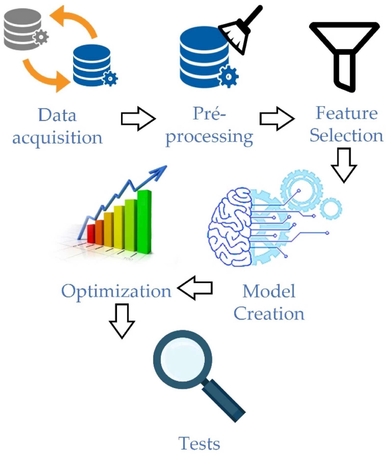
Figure 1 shows the steps proposed to carry out this work.
As shown in
Figure 1, the methodology implemented is composed of six sequential steps that aim to perform data processing, extract information, and select the most explanatory predictor features to forecast electricity consumption. Each step of the methodology will be described in detail below, as well as the tools used for its implementation.
3.1. Data Acquisition and Pre-Processing
The database used belongs to an individual consumer in the distribution network of the state of Paraiba, Brazil.
The analyzed consumer analyzed has a differentiated time-of-use tariff and is characterized by a maximum demand of up to 43 kW. A set of 1522 measurements performed every 30 min from 28 March 2019 to 29 April 2019 composes the database. The variables are presented in
Table 2.
As shown in
Table 2, the database is formed by a set of predictor variables and the objective variable. The predictor variables are composed of the time series of energy consumption measured every 30 min, hour, day, and rush hour. The objective variable, in turn, is the energy consumption to be forecast 30 min ahead.
Once the database is formed, a pre-processing step is performed, in which missing or possibly erroneous data is checked, and their correction is made. For the load time series, the wrong or missing data is replaced by an average of the consumption measured in the time before and after the error, as shown in (1). For errors in temporal variables, the correction is made from the information in the previous time interval.
where
is the corrected load,
is the load in the previous period and
is the load in the period after the error.
Still, during pre-processing, all variables are normalized in order to prevent the forecasting algorithm from becoming biased towards the variables of the highest order of magnitude. In this way, all information is transformed to be in the range of 0 and 1. In (2) the equation used for normalization is presented.
where
is the normalized variable,
is its actual value,
is the maximum value of the time series before normalization and
is the minimum value of the time series before normalization.
3.2. Feature Selection
In the feature selection stage, the database is analyzed to determine the information that most influences an accurate forecast of electricity consumption. For this, the database’s own information is used in addition to extracting new features that have the explanatory capacity for the forecasting task. This data mining process is called feature engineering and can be done by associating information present in the database or by mathematical relationships, as is the case with maximum and minimum daily consumption values, bringing new information to the predictor algorithm.
With a determined set of predictive features, the optimum set that maximizes the accuracy of the forecast must be selected. The tasks of extracting information and selecting the forecast set are performed following the steps indicated in the flowchart of
Figure 2.
As shown in
Figure 2, the first step in determining the forecast set is to analyze the database with the objective of extracting as much information as possible to assist in the prediction of electricity consumption. For this purpose, the features presented in
Table 3 are calculated, which statistically evaluate the time series of energy consumption in terms of position, dispersion, and distribution.
As a short-term load forecast is sought, only the set of data measured in the last 12 h is considered for the calculation of the features in
Table 3. Thus, only short-term information is attributed to these features. The new information is added to the database for further analysis.
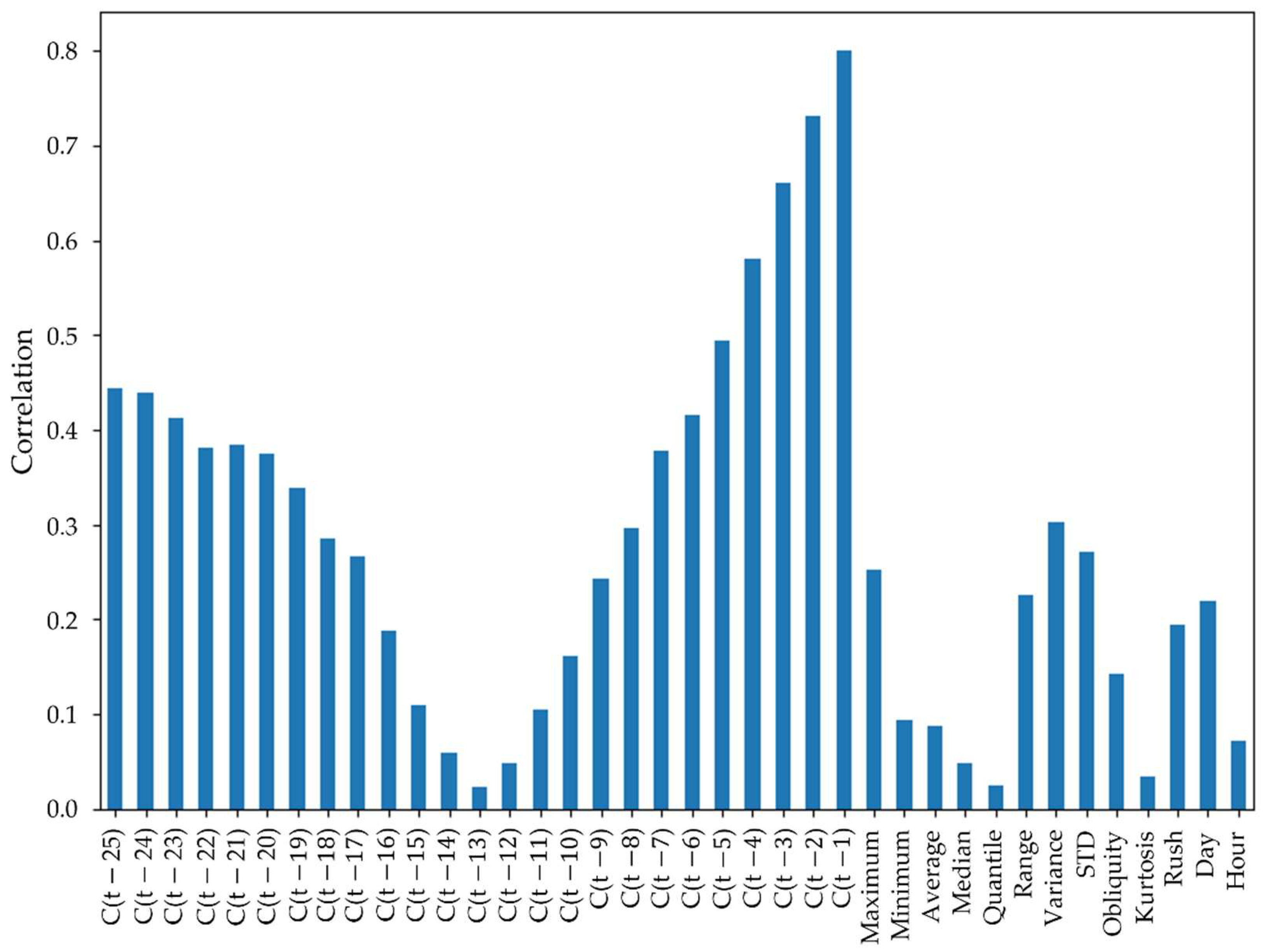
The next step in selecting the features is to determine which information has the greatest explanatory capacity for forecasting energy consumption. This is accomplished by analyzing the correlation and mutual information (MI) of the features in the database.
The correlation between the features of the database and the energy consumption forecast is calculated with the objective of discarding features that have a weak correlation, which possibly indicates that the information will not be relevant to the forecast model or, even, will harm the results.
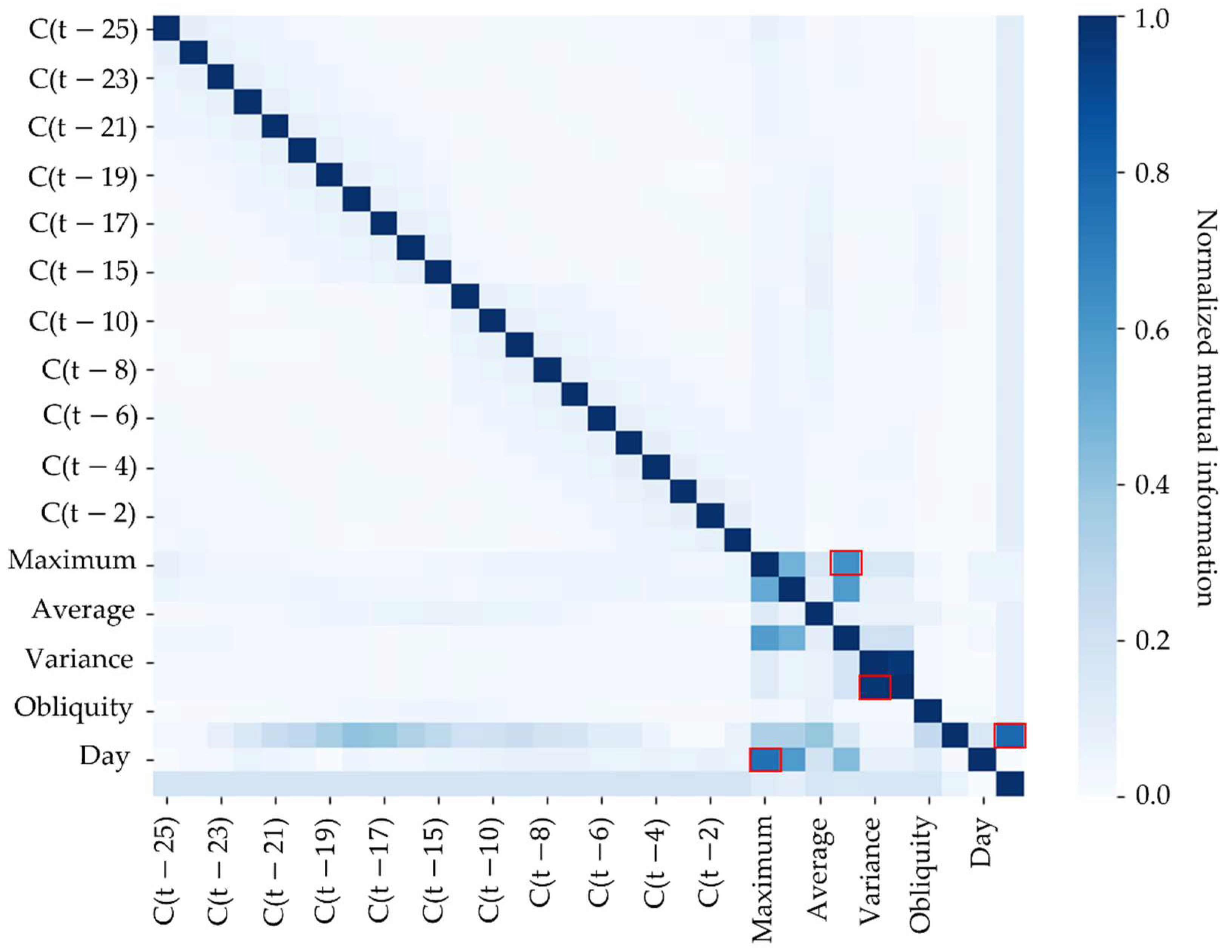
Finally, the mutual information (MI) analysis is performed among the remaining features. Mutual information is a measure of similarity that determines the amount of information that a variable contains about another and that, unlike correlation, could identify both linear and non-linear relationships [
24]. Thus, the features are analyzed concerning MI to identify redundancies in the database, keeping only those that have a higher MI with the objective variable. The criterion adopted for a pair of features to be considered redundant is to be greater than 0.6, thus, more than half of the information that the variables have is the same.
Thus, after the extraction and analysis of the features, the forecast set chosen must be formed by variables loosely linked to each other, that is, that individually bring new information to the forecast system, and that have a high explanatory capacity in relation to the forecast.
3.3. Model Creation
After the procedures described above, the database formed can be submitted to a model based on machine learning to perform the load forecast.
Four forecasting models using the main forecasting techniques found in the scientific bibliography were implemented. These are:
Support vector regression (SVR);
Feedforward multilayer perceptron (MLP);
Long short-term memory (LSTM);
ARTMAP-Fuzzy.
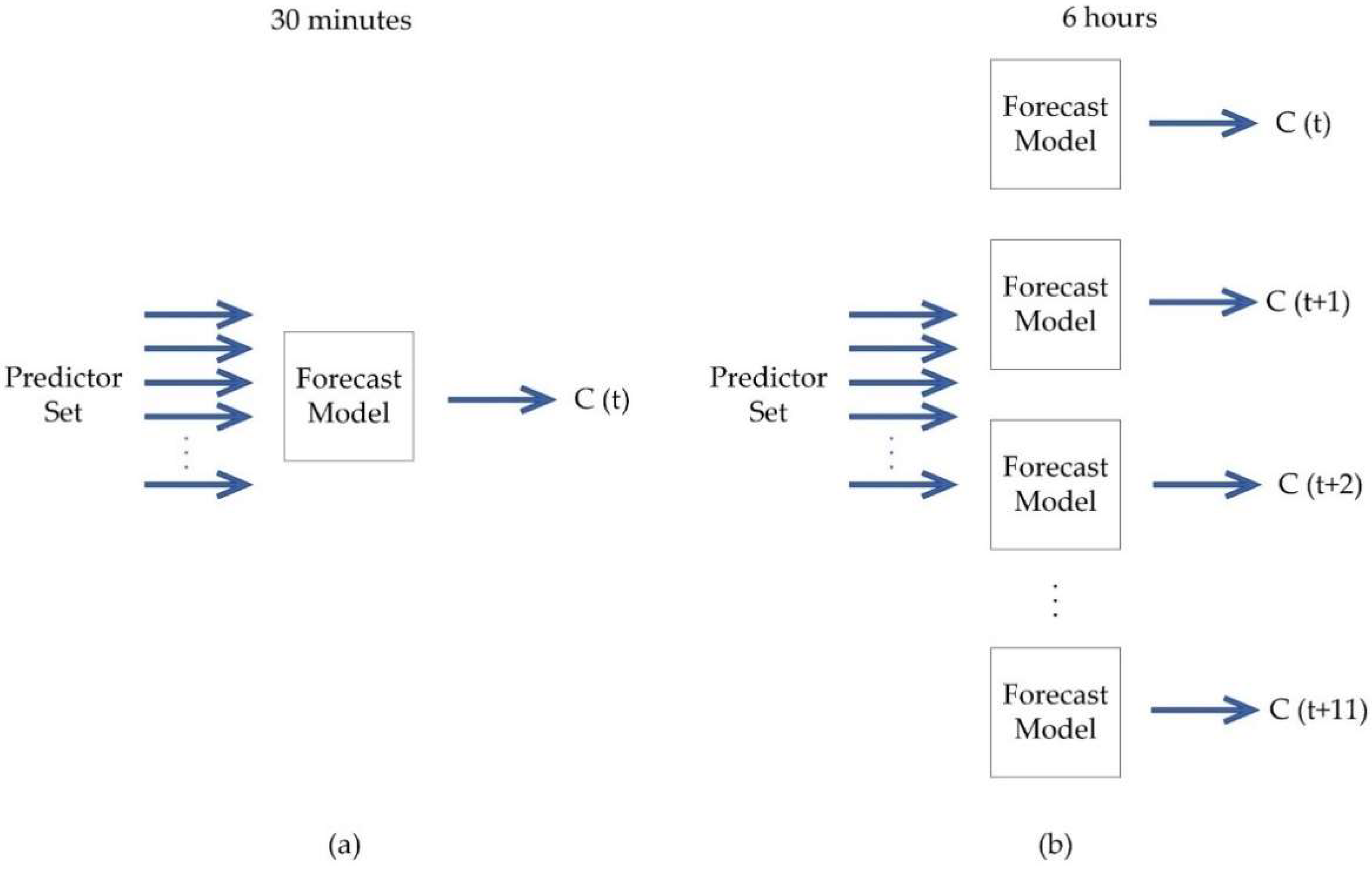
Forecasting models were created with a 30-min and 6-h horizon (with a 30-min step between predictions). Due to the differences found between the techniques, the models created with the MLP and LSTM networks differ from the others during the forecast with a 6-h horizon.
Figure 3 and
Figure 4 show the ways chosen to use the forecast models according to their limitations.
As can be seen in
Figure 3 and
Figure 4, when using SVR or the ARTMAP-Fuzzy network, a model is trained for each output. In another way, for the MLP and LSTM neural networks, which have the output formed by neurons, only one model can be trained with the number of neurons required for the desired output, as shown in
Figure 4.
The database was separated into two sets (75% and 25%) for each predictor system, where 75% of the data is used for training and 25% is used for testing and validation.
3.4. Optimization
The models described in the previous subsection require the definition of hyperparameters during their implementation. Hyperparameters quantify properties of predictive systems that are constant throughout the database samples and that condition and establish non-linear relationships with the other parameters [
25]. In other words, it can be said that hyperparameters are the initial configurations given to the forecasting system, defined from the previously known characteristics of the database.
A good choice of hyperparameters has a great influence on the performance of the predictive model. For this, there are several search techniques with the function of determining the optimal set for a model. One that can be implemented and that is suitable for searches with few variables is the randomized optimization of parameters [
26].
From a defined set of hyperparameters and a specified search range, the randomized parameter optimization method (RPO) tests the predictor system by varying the hyperparameters within a probabilistic distribution, until the most accurate models are found.
The RPO is used to determine the best set of hyperparameters for the four models described in the previous subsection.
Table 4 shows the defined hyperparameters to be optimized, the search limit and the number of interactions performed.
The choice of the search limits takes into account the optimal value expected for each hyperparameter according to the typical values found in the literature. Some hyperparameters were set with typical values used for time series forecasting, as shown in
Table 5 [
27,
28].
With the definition of hyperparameters, the predictive models are ready to be trained and used.
3.5. Tests
The evaluation of a regressive predictor model requires the use of metrics that verify the robustness of the solution, indicating how close the model is to reality. Essentially, the performance metric must be taken into account the individual error of each forecast and the model’s deviation from real values. For this, there are several metrics consolidated in statistics and data science. Some of the main ones are the mean absolute percentage error (MAPE), which offers a measure of the error of all estimates made by the model, and the coefficient of determination (R2), which indicates how fitted the model is in relation to the real values.
MAPE is a measure of the accuracy of a model that considers each estimate error. The
MAPE result ranges from 0 to 100, indicating that the model is more accurate the lower its value. The calculation is defined, as the name implies, by the average percentage error of all estimates, as shown in (3).
where
are the model estimates,
are the real values and
is the size of the vector
.
The coefficient of determination (
R2), in turn, is a metric for determining the fit of a model to real values. Its result ranges from 0 to 1 and indicates that the model is more accurate the higher its result. Its calculation is performed as shown in (4).
where,
are the model estimates,
are the real values and
is the average value of all measurements.
The error assessment metrics implemented in this work will be the MAPE and the R2 coefficient. The objective is to determine the model that presents the best results in relation to the forecast accuracy.
5. Conclusions
In this paper, a methodology was developed to extract and select the best set of attributes in short-term load forecasting. The extraction of attributes from a database was carried out from a statistical analysis taking into account the position, dispersion, and distribution of the time series. The selection process was carried out through correlation analysis and MI, indicating a set of explanatory and independent features. The methodology was applied together to 4 (four) of the well-known time series forecasting techniques in order to predict the consumption of an individual consumer.
The results obtained indicate an improvement in the short-term load forecasting of individual consumers. The forecast error (MAPE) decreased by 19.8% and the curve fitting (R2) increased by 36.31% in the best case (SVR) when compared to the baseline approach.
Taking into account only the extraction and selection of attributes and keeping forecasting techniques constant, an improvement of 1.78% was achieved in the 30-min horizon and 2.37% in the 6-h horizon of load forecasting. In this way, it can be said that the selected dataset contributed to the improvement of the final models, making clear the contribution and importance of the treatment and selection of features from the database for a correct forecast of energy consumption.
The methodology implemented has the limitation of requiring the determination of limits of importance for the feature selection, both for correlation and for MI. This limitation can affect the accuracy of prediction models due to the need for specialized human intervention, which also makes scalability difficult. In future works, optimization techniques may be proposed that determine the best values without the need for intervention.
The prediction of very random loads, such as the individual consumer analyzed in this paper, is still emerging research, but it has great potential in the optimization of the electrical system. We consider that the results presented in this paper contribute to the development of the area and growth of the characterization of the consumer profile.


