
Impact of Solar Thermal Energy on the Energy Matrix under Equatorial Andean Context

 , ,
, ,
Abstract
:1. Introduction
1.1. Characteristics of Low-Temperature ST Systems
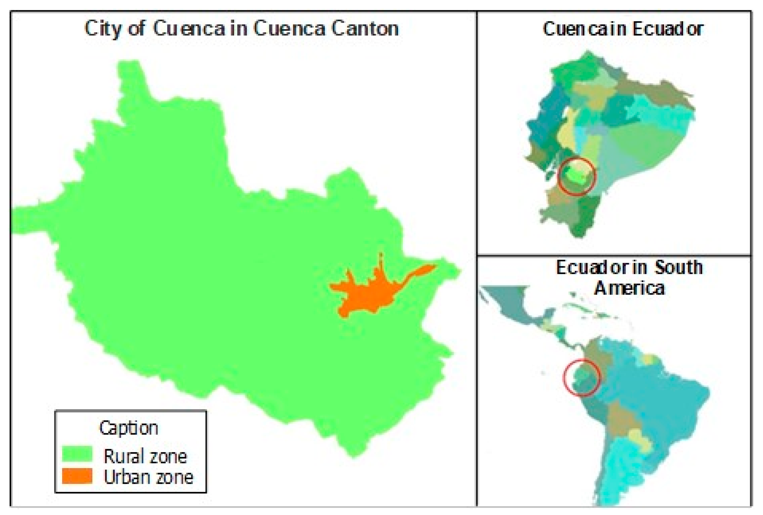
1.2. The Intermediate City of Cuenca
2. Materials and Methods
2.1. Scenarios
2.2. Sustainability Indicators Used to Measure the Impact of the Use of ST Heaters for DHW in the City of Cuenca
2.2.1. Energy Autarchy
- EA is the autarky [%],
- IEp indicates primary energy imports (BOE),
- IEs indicates secondary energy imports (BOE), n is the number of primary energy forms, and m is the number of secondary energy forms.
- ES is the gross domestic energy supply (endogenous energy + primary energy imports + primary energy imports-primary energy exports-secondary energy exports) (BOE).
2.2.2. Energy Price
- PEj is the energy price j [USD $/BOE],
- Ce is the cost of energy production during its useful life [USD $/BOE],
- Pr is the business profit [%], and
- Tx indicates taxes [%].
2.2.3. Cost of Energy Production
- Ce is energy production cost during its useful life [USD/kWh],
- Inv is the investment in the year (including interest during construction and all auxiliary elements and electrical infrastructure) [USD/kW],
- O&M represents operation and maintenance cost per year t [USD/kWh],
- r is the discount rate,
- Eth is the energy produced in year t [kWh], and
- t indicates the years of operation of the plant.
2.2.4. Mean Price of Energy to the Final Consumer
- PE is the mean energy price [USD $/BOE],
- PEjk is the price of energy k in sector j [USD $/BOE],
- Ejk is the amount of energy of energy k in sector j [BOE],
- m is the number of consumption sectors, and
- n is the number of energy forms.
2.2.5. Use of RE in the Total Energy Supply
- UR is the share of RE in the total energy supply [%],
- REi is the supply of RE i [BOE],
- ES is the gross domestic energy supply [BOE], and
- m is the number of renewable energy production technologies.
2.2.6. Use of RE in the Supply of Electricity
- URe is the participation of the RE in electric energy production [BOE],
- REe is the production of electricity using RE with i [BOE] technology,
- ESe represents the electrical energy requirements in [BOE], and
- m is the number of electrical energy production technologies with RE technologies.
2.2.7. Relative Purity of Energy Use
- PRe is the energy purity [ton CO2/BOE],
- CEC represents the carbon dioxide emissions related to energy demand [ton CO2],
- ED is the total energy demand [BOE], and
- m is the energy required in the city.
- ALn,j,i is the activity level related to fuel type n, equipment j, and sector i;
- EFn,j,i is the emissions factor related to fuel type n, equipment j, and sector I; and
- EFt,m,s is the emissions factor related to the primary fuel type used to produce secondary energy type t using equipment type j.
2.2.8. Employment
- Em represents the jobs per year in the energy industry,
- Di is the energy demand i [BOE], and
- fei is the energy use Factor i [jobs-year/BE].
3. Results
- Eth is the heat energy demand to heat water (kJ/year),
- Q is DHW consumed (L/day),
- ρa is water density (kg/L),
- Ce is the specific heat of water (4.18 kJ/kg°C),
- Tuse is the temperature at which the water is to be supplied (°C),
- Tnetw is the water network temperature (°C), and
- n is the number of days per year (days).
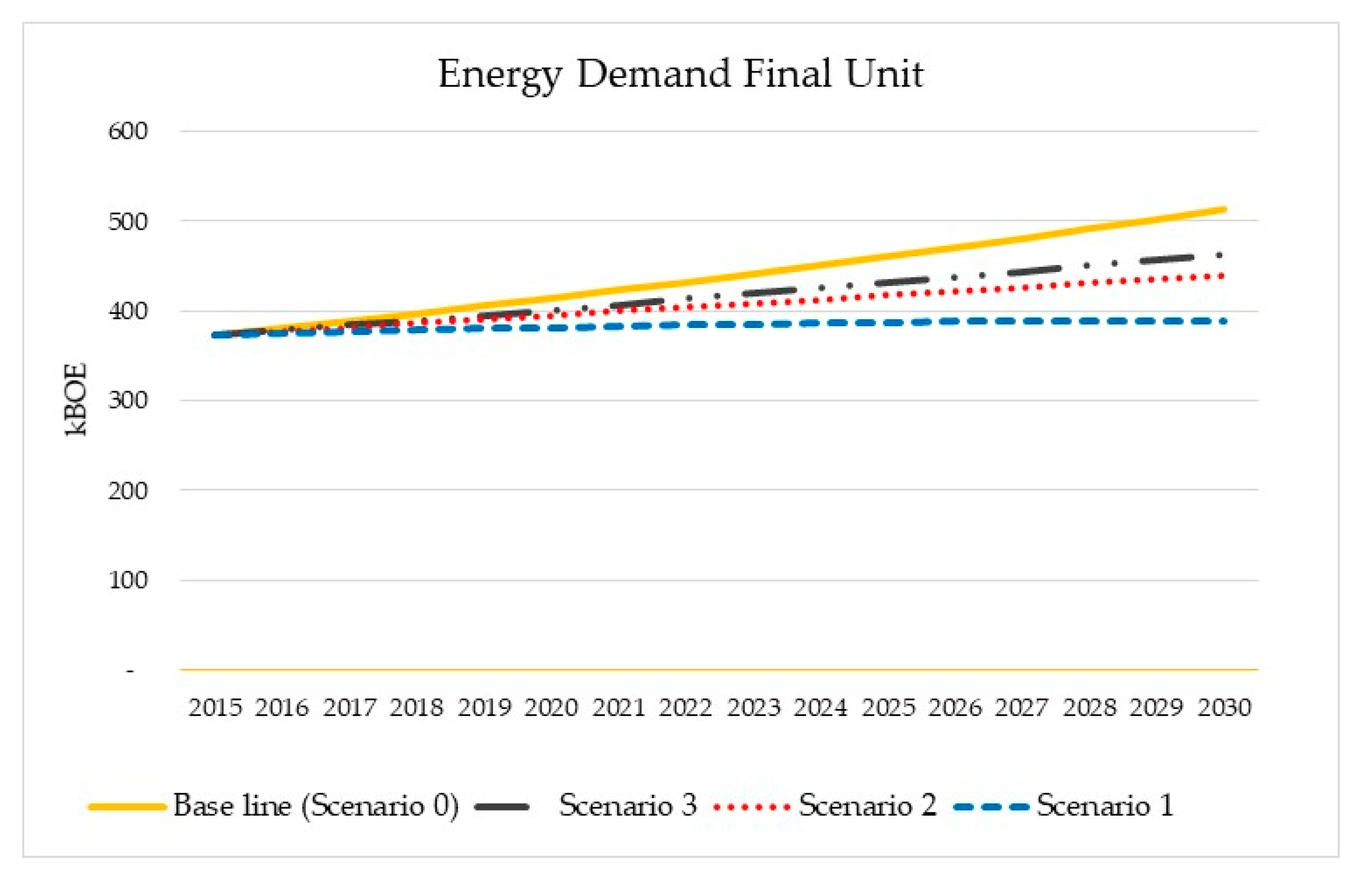
3.1. Scenarios and Prospects
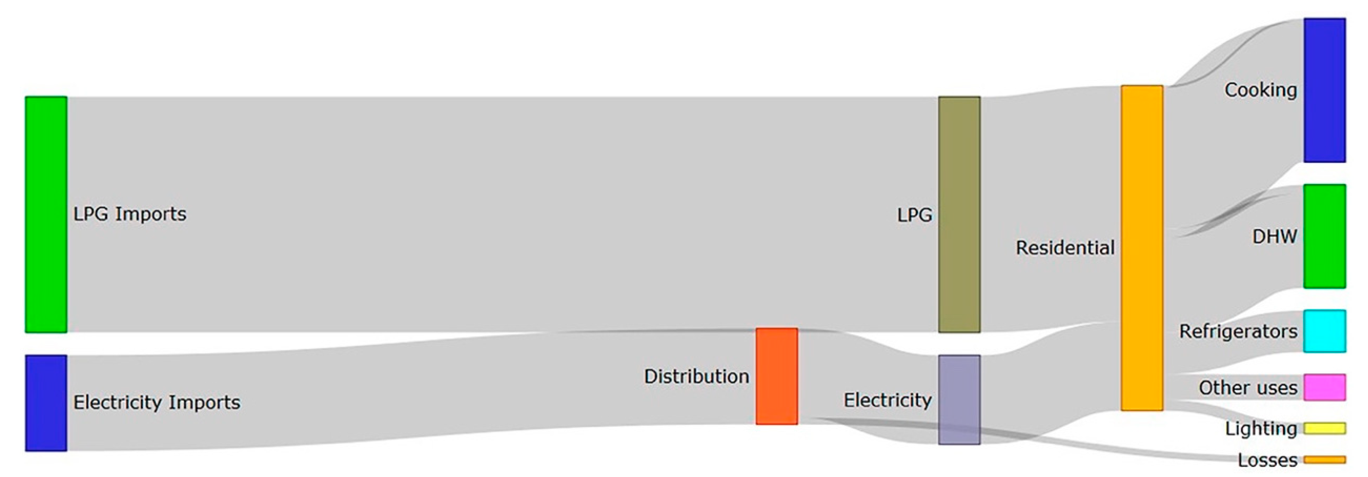
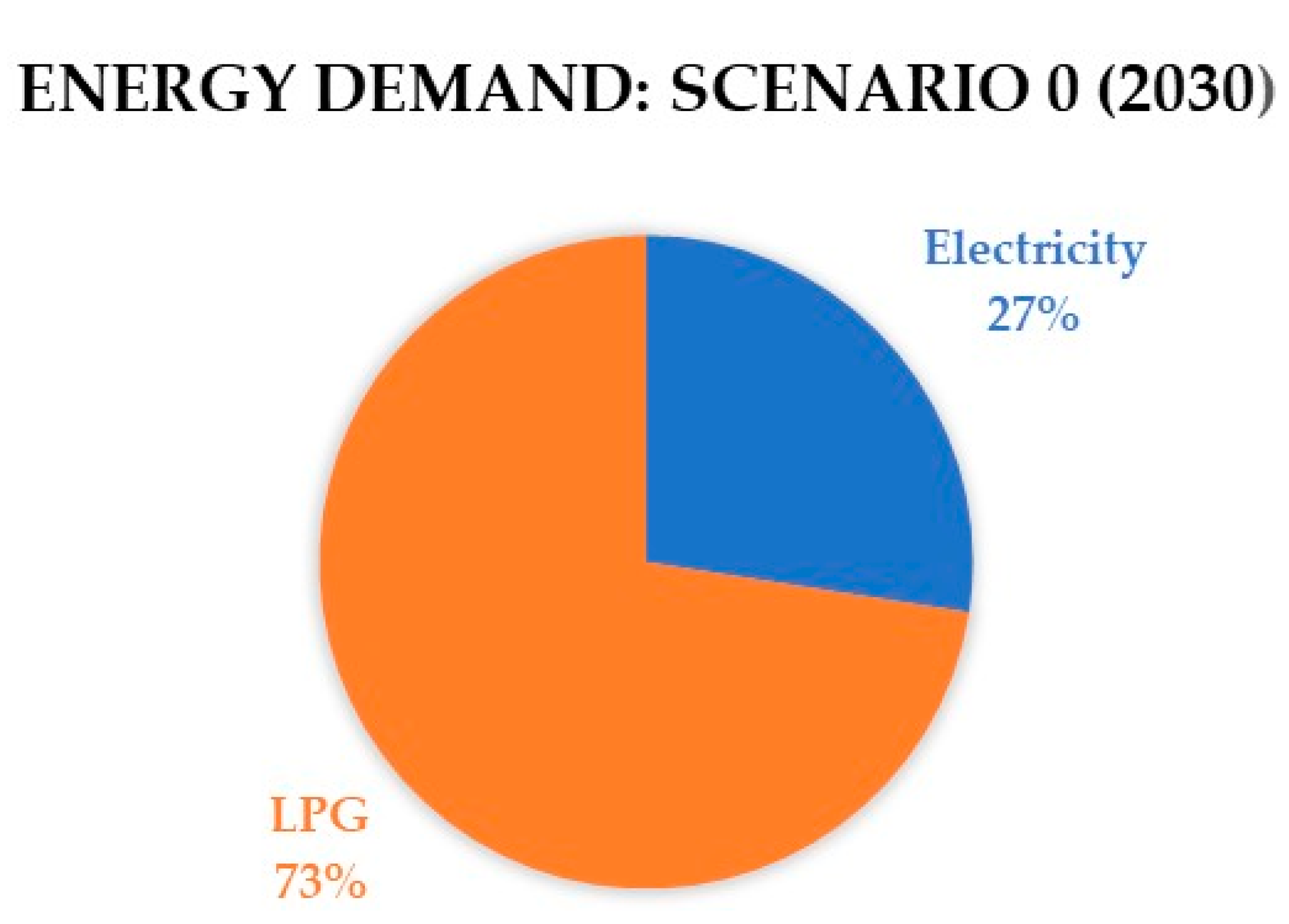
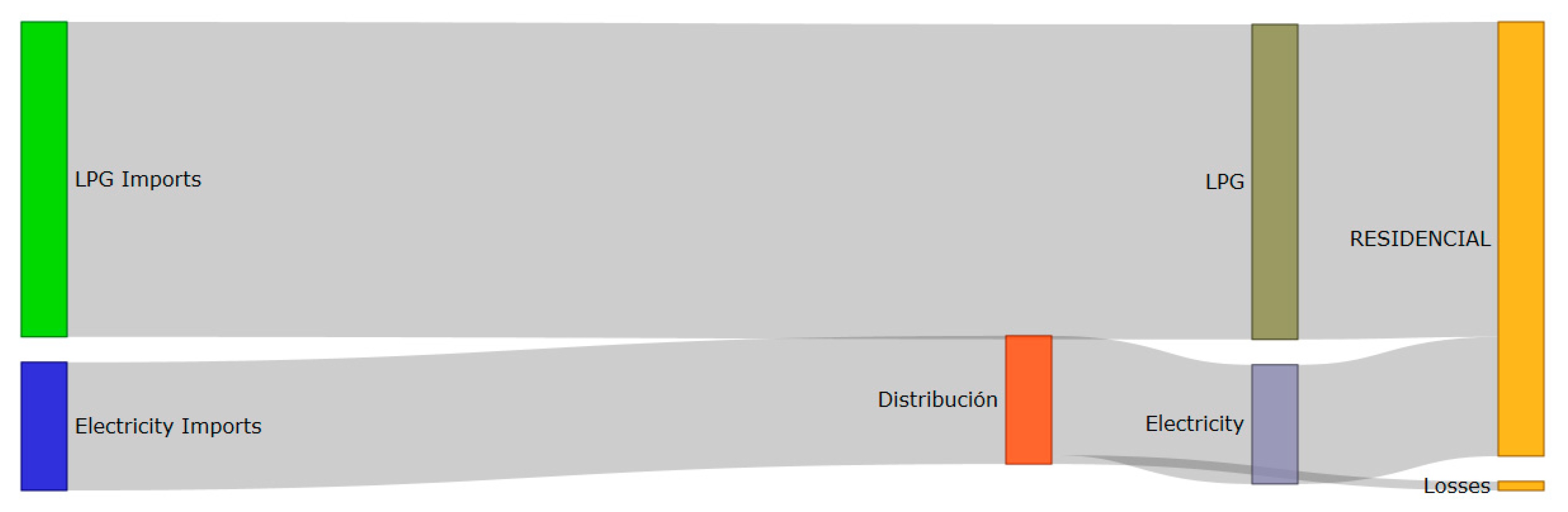
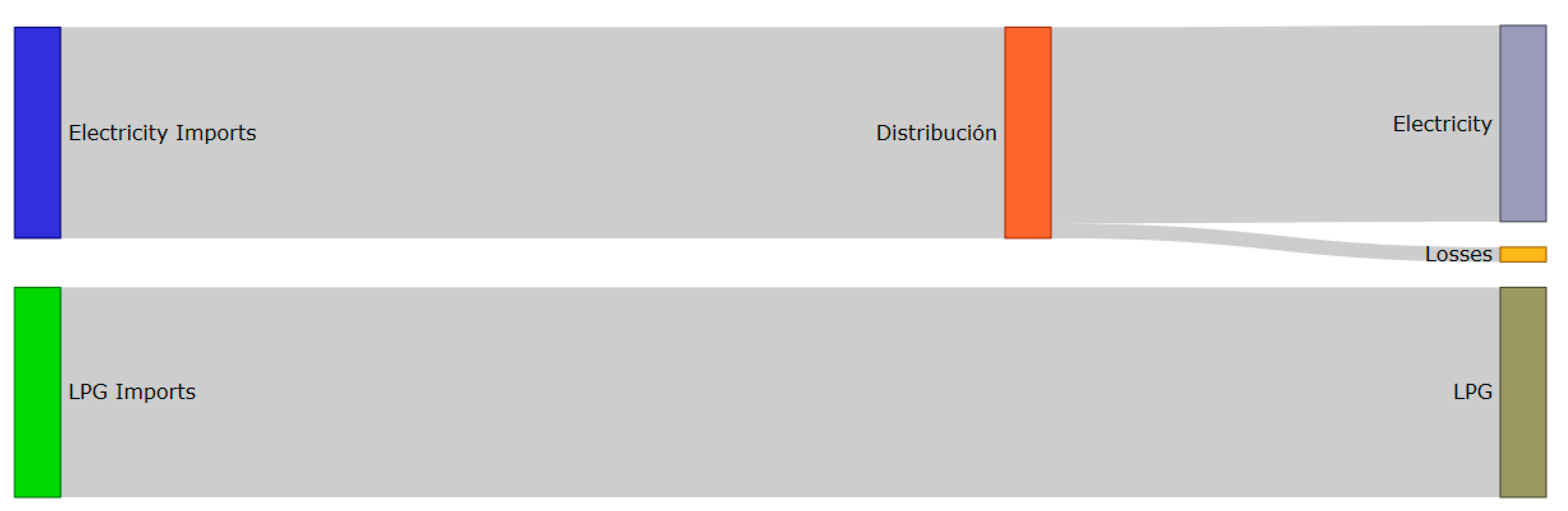
3.1.1. Baseline
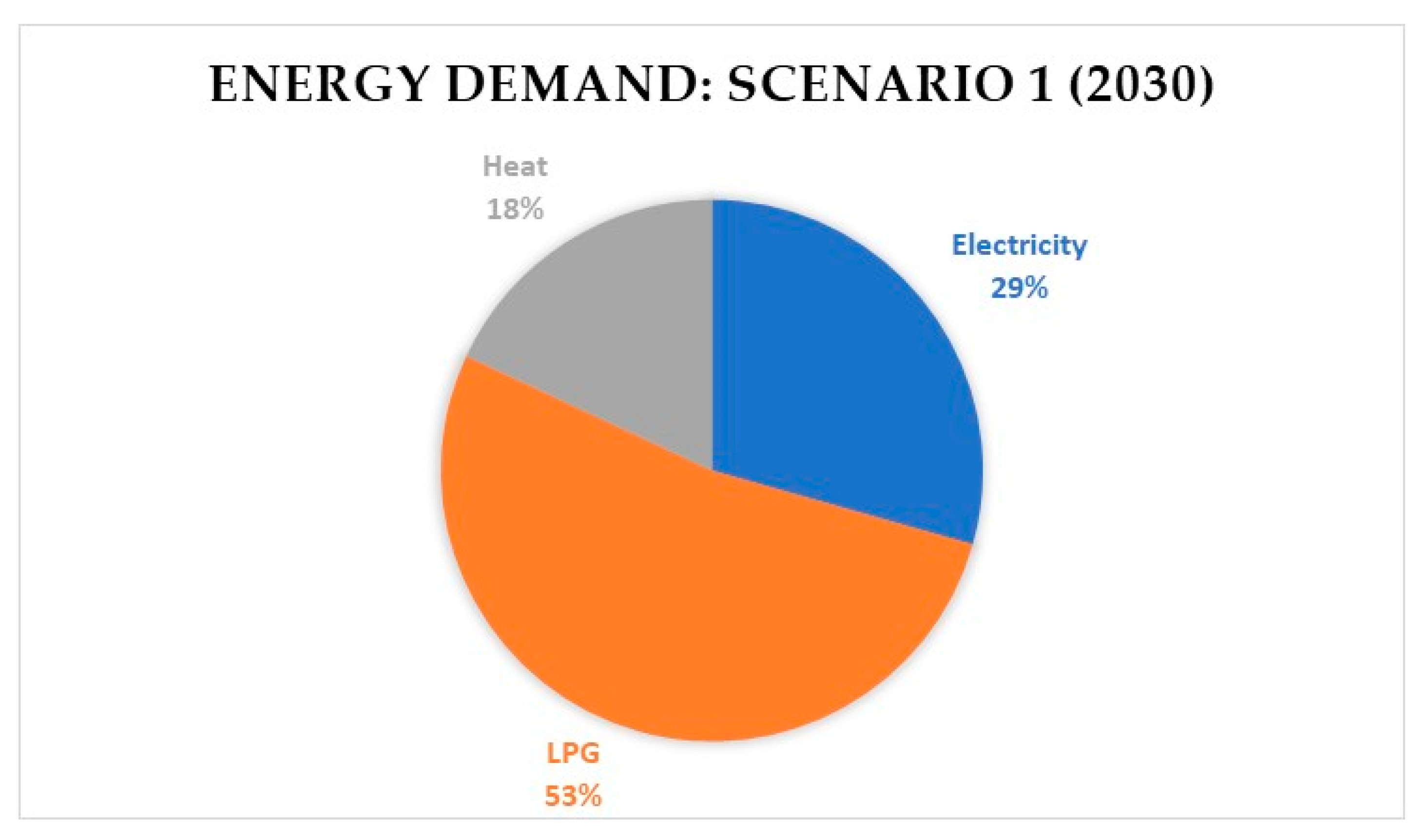
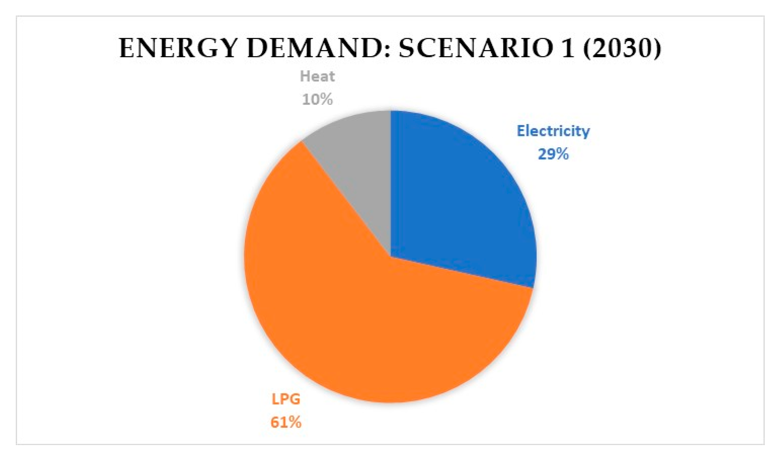
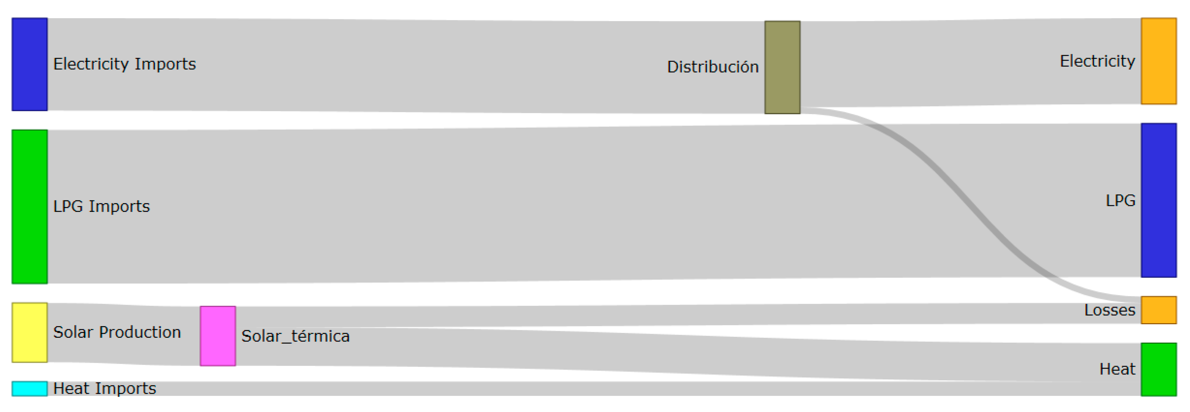
3.1.2. Scenarios for the Adoption of ST Systems in the Urban Area of Cuenca


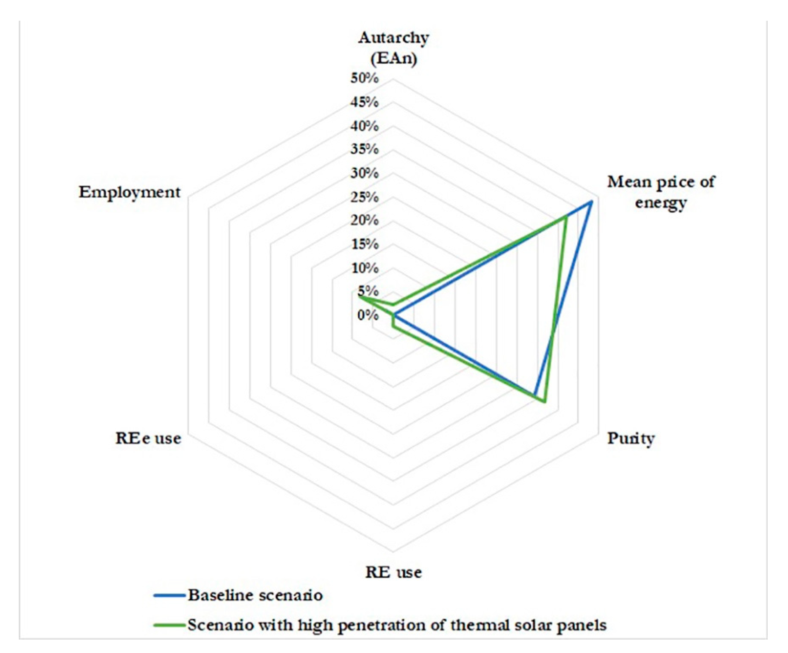
3.1.3. Calculation of Sustainability Indicators
Autarchy
Energy Price
Mean Price of Energy to the Final Consumer
Use of RE in the Total Energy Supply
Use of RE in the Supply of Electricity
Purity of Energy
Employment
- CIMI is the number of people required for the construction, installation, and manufacture of a reference plant [person-years];
- NI is the number of years used for MIC of the reference facility [years];
- PI is the power size of the reference installation [MW]; and
- CIM is the number of people employed in the construction of a reference infrastructure MW during NI years [people-year/MW].
- OMI is the number of jobs required for the operation and maintenance of a reference facility in one year [jobs-year] an
- PI is the power production of the reference installation [MW].
- Ie is the employment indicator for a renewable technology [total jobs-year/GWh],
- t is the lifetime of the renewable technology [years], and
- Fp is the plant factor of the renewable technology.
3.1.4. Amortization of ST with and without Subsidy
4. Discussion
5. Conclusions
Author Contributions
Funding
Data Availability Statement
Acknowledgments
Conflicts of Interest
References
- Cristofari, C.; Carutasiu, M.B.; Canaletti, J.L.; Norvaišienė, R.; Motte, F.; Notton, G. Building integration of solar thermal systems-example of a refurbishment of a church rectory. Renew. Energy 2019, 137, 67–81. [Google Scholar] [CrossRef]
- Kalogirou, S.A. Solar thermal collectors and applications. Prog. Energy Combust. Sci. 2004, 30, 231–295. [Google Scholar] [CrossRef]
- Ameer, S.A.A. State of the Art of Solar Absorption Cooling Technologies. Int. J. Res. Appl. Sci. Eng. Technol. 2017, 5, 84–98. [Google Scholar] [CrossRef]
- Benli, H. Potential application of solar water heaters for hot water production in Turkey. Renew. Sustain. Energy Rev. 2016, 54, 99–109. [Google Scholar] [CrossRef]
- Rosas-Flores, J.A.; Rosas-Flores, D.; Zayas, J.L.F. Potential energy saving in urban and rural households of Mexico by use of solar water heaters, using geographical information system. Renew. Sustain. Energy Rev. 2016, 53, 243–252. [Google Scholar] [CrossRef]
- Han, J.; Mol, A.P.J.; Lu, Y. Solar water heaters in China: A new day dawning. Energy Policy 2010, 38, 383–391. [Google Scholar] [CrossRef]
- IDEA. Plan de Energias Renovables. 2011, pp. 1–824. Available online: https://www.idae.es/tecnologias/energias-renovables/plan-de-energias-renovables-2011-2020/estudios-de-apoyo-la.Detalle (accessed on 31 July 2022).
- Greening, B.; Azapagic, A. Domestic solar thermal water heating: A sustainable option for theUK? Renew. Energy 2014, 63, 23–36. [Google Scholar] [CrossRef]
- IRENA. Solar Heating and Cooling for Residential Applications Technology Brief. Abu Dhabi, EAU. 2015. Available online: https://www.irena.org/publications/2015/Jan/Solar-Heating-and-Cooling-for-Residential-Applications (accessed on 31 July 2022).
- Izquierdo, S.; Montañés, C.; Dopazo, C.; Fueyo, N. Roof-top solar energy potential under performance-based building energy codes: The case of Spain. Sol. Energy 2011, 85, 208–213. [Google Scholar] [CrossRef]
- Marique, A.-F.; Reiter, S. A simplified framework to assess the feasibility of zero-energy at the neighbourhood/community scale. Energy Build. 2014, 82, 114–122. [Google Scholar] [CrossRef] [Green Version]
- Kanters, J.; Wall, M.; Dubois, M.-C. Typical Values for Active Solar Energy in Urban Planning. Energy Procedia 2014, 48, 1607–1616. [Google Scholar] [CrossRef] [Green Version]
- Zalamea-Leon, E.; García-Alvarado, R. Roof characteristics for integrated solar collection in dwellings of Real-Estate developments in Concepción, Chile. J. Constr. 2014, 36, 36–44. [Google Scholar]
- Creamer-Guillen, B.; Becerra-Robalino, R. Cuantificación de los Subsidios de Derivados del Petróleo a los Hidrocarburos en el Ecuador. Bol. Estadístico del Sect. Hidrocarb. 2016, 2, 9–26. [Google Scholar]
- Jaisankar, S.; Ananth, J.; Thulasi, S.; Jayasuthakar, S.T.; Sheeba, K.N. A comprehensive review on solar water heaters. Renew. Sustain. Energy Rev. 2011, 15, 3045–3050. [Google Scholar] [CrossRef]
- Islam, M.R.; Sumathy, K.; Ullah, S. Solar water heating systems and their market trends. Renew. Sustain. Energy Rev. 2013, 17, 1–25. [Google Scholar] [CrossRef]
- Suter, J.-M.; Letz, T.; Weiss, W. Solar Combisystems—Overview. 2003. Available online: http://www.bfe.admin.ch/php/modules/publikationen/stream.php?extlang=en&name=en_168325772.pdf (accessed on 31 July 2022).
- Hazami, M.; Naili, N.; Attar, I.; Farhat, A. Solar water heating systems feasibility for domestic requests in Tunisia: Thermal potential and economic analysis. Energy Convers. Manag. 2013, 76, 599–608. [Google Scholar] [CrossRef]
- Ma, B.; Song, G.; Smardon, R.C.; Chen, J. Diffusion of solar water heaters in regional China: Economic feasibility and policy effectiveness evaluation. Energy Policy 2014, 72, 23–34. [Google Scholar] [CrossRef]
- SHIP. Database for applications of solar heat integration in industrial processes. In Solar Heat for Industrial Processes; ETSAP and IRENA: Abu Dhabi, United Arab Emirates, 2017. [Google Scholar]
- Pincetl, S.; Bunje, P.; Holmes, T. An expanded urban metabolism method: Toward a systems approach for assessing urban energy processes and causes. Landsc. Urban Plan. 2012, 107, 193–202. [Google Scholar] [CrossRef]
- Masruroh, N.A.; Li, B.; Klemeš, J. Life cycle analysis of a solar thermal system with thermochemical storage process. Renew. Energy 2006, 31, 537–548. [Google Scholar] [CrossRef]
- Lamnatou, C.; Chemisana, D.; Mateus, R.; Almeida, M.G.; Silva, S.M. Review and perspectives on life cycle analysis of solar technologies with emphasis on building-integrated solar thermal systems. Renew. Energy 2015, 75, 833–846. [Google Scholar] [CrossRef]
- GHK and Bio Intelligence Service. A Study to Examine the Costs and Benefits of the ELV Directive—Final Report. no. May 2006, p. 190. 2006. Available online: http://ec.europa.eu/environment/waste/pdf/study/final_report.pdf (accessed on 31 July 2022).
- GAD Municipal de Cuenca. Ciudades Intermedias, Crecimiento y Renovación Urbana. In Proceedings of the Thematic Meeting, Intermediate Cities, Cuenca, Ecuador, 9–11 November 2015; p. 27. [Google Scholar]
- GAD Cuenca. Plan de Desarrollo y Ordenamiento Territorial del Cantón Cuenca; GAD: Cuenca, Ecuador, 2015.
- BID Cuenca. Ciudad Sostenible: Plan de Acción; BID: Cuenca, Ecuador, 2014. [Google Scholar]
- Universidad de Cuenca. Vivienda Sustentable y Segura; Universidad de Cuenca: Cuenca, Ecuador, 2017. [Google Scholar]
- Lozano, M.F.L. Explotación del Gas Natural en el Sector Fabril del Parque Industrial de Cuenca; Universidad de Cuenca: Cuenca, Ecuador, 2014. [Google Scholar]
- Mogrovejo, W.F.; Sarmiento, J. Análisis de Factibilidad Técnica y Económica en la Implementación de Energía Fotovoltaica y Termo Solar Para Generación de Electricidad y Calentamiento de Agua Mediante Paneles Solares Fijos y con un Seguidor de sol de Construcción Casera, Para una Vivien; Universidad de Cuenca: Cuenca, Ecuador, 2011. [Google Scholar]
- Calle-Siguencia, J.; Tinoco-Gómez, Ó. Obtención de ACS con energía solar en el cantón Cuenca y análisis de la contaminación ambiental Obtaining of SHW with solar energy in the canton cuenca and analysis of environmental pollution. Ingenius 2018, 19, 89–101. [Google Scholar] [CrossRef]
- INER. Escenarios de Prospectiva Energética Para Ecuador a 2050; INER: Quito, Ecuador, 2016.
- Barragán Escandon, A. El Autoabastecimiento Energético en los Países en vías de Desarrollo en el Marco del Metabolismo Urbano; Universidad de Jaén: Caso Cuenca, Ecuador, 2018. [Google Scholar]
- Barragán-Escandón, A.; Zalamea-León, E.; Terrados-Cepeda, J. Incidence of photovoltaics in cities based on indicators of occupancy and urban sustainability. Energies 2019, 12, 810. [Google Scholar] [CrossRef] [Green Version]
- OLADE. Manual de Planificación Energética; OLADE: Quito, Ecuador, 2014. [Google Scholar]
- MEER. Elaboración de la Prospectiva Energética del del Ecuador 2012–2040; MEER: Quito, Ecuador, 2015. [Google Scholar]
- MICSE. Balance Energético Nacional 2016, Año Base 2015; MICSE: Quito, Ecuador, 2015.
- OECD/IEA. Energy Efficiency Indicators: Essentials for Policy Making; OECD/IEA: Paris, France, 2014. [Google Scholar]
- CEPAL/OLADE/GTZ. Energía y Desarrollo Sustentable en América Latina y el Caribe: Guía Para la Formulación de Políticas Energéticas; Naciones Unidas: Santiago, Chile, 2003. [Google Scholar]
- Garcia, G.; Hernández, F.; Luna, N. Manual de Estadísticas Energéticas; Organización Latinoamericana de Energía: Quito, Ecuador, 2011; Volume 53. [Google Scholar]
- Zhang, L.; Feng, Y.; Chen, B. Alternative scenarios for the development of a low-carbon city: A case study of Beijing, China. Energies 2011, 4, 2295–2310. [Google Scholar] [CrossRef]
- Heaps, C.G. Long-Range Energy Alternatives Planning (LEAP) System, Software version: 2017.0.11; Stockholm Environment Institute: Somerville, MA, USA, 2016; Available online: https://www.energycommunity.org (accessed on 31 July 2022).
- Martinez, P. Usos Finales de Energía Eléctrica y GLP en el Cantón Cuenca. Escenarios al año 2015; Universidad de Cuenca: Cuenca, Ecuador, 2010. [Google Scholar]
- IDEE. Balances Energéticos. In Seminario-Taller Política Energética para el Desarrollo Sustentable y el uso del Modelo LEAP, 15th ed.; Fundación Bariloche: Bariloche, Argentina, 2016; p. 106. [Google Scholar]
- ARCH-Azuay and Centrosur. Base de Datos; ARCH-Azuay and Centrosur: Cuenca, Ecuador, 2017. [Google Scholar]
- Universidad del Azuay. Ordenamiento Territorial Del Canton Cuenca; Universidad del Azuay: Azuay, Ecuador, 2012; p. 335. [Google Scholar]
- Joubert, E.C.; Hess, S.; van Niekerk, J.L. Large-scale solar water heating in South Africa: Status, barriers and recommendations. Renew. Energy 2016, 97, 809–822. [Google Scholar] [CrossRef]
- Araujo, A. Alza de Tarifas Eléctricas Busca Rebajar el Subsidio; Diario el Comercio: Quito, Ecuador, 2014. [Google Scholar]
- Ponce-Jara, M.A.; Castro, M.; Pelaez-Samaniego, M.R.; Espinoza-Abad, J.L.; Ruiz, E. Electricity sector in Ecuador: An overview of the 2007–2017 decade. Energy Policy 2018, 113, 513–522. [Google Scholar] [CrossRef]
- Petroecuador. Precios de Venta a Nivel de Terminal para las Comercializadoras Calificadas y Autorizadas a Nivel Nacional Periodo; Petroecuador: Quito, Ecuador, 2016. [Google Scholar]
- Rutovitz, J.; Dominish, E.; Downes, J. Calculating Global Energy Sector Jobs 2015 Methodology Update; Institute for Sustainable Futures: Ultimo, Australia, 2015. [Google Scholar]
- Rutovitz, J. South African Energy Sector Jobs to 2030; Greenpeace Africa: Randburg, South Africa, 2010. [Google Scholar]
- Ren21. The First Decade: 2004–2014, 10 Years of Renewable Energy Progress; Ren21: Paris, France, 2014. [Google Scholar]
- Wei, M.; Patadia, S.; Kammen, D.M. Putting renewables and energy efficiency to work: How many jobs can the clean energy industry generate in the US? Energy Policy 2010, 38, 919–931. [Google Scholar] [CrossRef]


| City | Potential | Demand | Use | Reference | Objective of the Study |
|---|---|---|---|---|---|
| Mexico (urban residential areas) | 45.60% | 29,088 GWh/year | Thermal | [5] | Evaluates the solar potential for water heating. |
| Spain (8005 municipalities) | 68.40% | 28,249.00 GWh/year | Thermal | [10] | Determines the roof surface available for the placement of thermal solar panels. |
| Concepción, Chile (3233 dwellings) | 75.00% | 19,788.70 MWh | Thermal | [13] | Determines the hip-end with the best suitability per dwelling according to orientation and inclination; compares joint feasible production in the area of study against typical demands. |
| Efficiency (%) | Source |
|---|---|
| 70 | [15] |
| 80 | [10] |
| 35 | [8] |
| 65 to 70 Flat plate collector | [7] |
| 70 to 75 Evacuated tube collector | [7] |
| System | Investment Costs | Reference |
|---|---|---|
| Solar water heaters | 546 USD/kW | [4] |
| Thermosiphon flat plate collector | ||
| 1.4 kW *–2 m2) | ||
| 502 USD/kW | [4] | |
| Direct without pump | ||
| 1.3 kW–1.85 m2 | ||
| 440 USD/kW | [5] | |
| Direct thermosiphon | ||
| 2.48 kW–3.55 m2 | ||
| 671 USD/kW | [16] | |
| Thermosiphon flat plate collector | ||
| 1.4 kW–2 m2 | ||
| 300 USD/kW ** | [9] | |
| Thermosiphon evacuated tube collectors | ||
| 1.05 kW–1.05 m2 | ||
| 786 USD/kW | [18] | |
| Direct thermosiphon evacuated tube collector 1.4 kW–2 m2 | ||
| Solar water heaters | 2309 USD/kW | [19] |
| Indirect with pump 3.24 kW * | ||
| 2150 USD/kW | [18] | |
| Indirect with pump 3.85 kW | ||
| 790 USD/kW | [16] | |
| Direct with pump 2.3 kW | ||
| 1120 USD/kW | [9] | |
| Flat plate collector 10 kW | ||
| 854 USD/kW | [9] | |
| Flat plate collector less than 20 kW **** | ||
| 649 | [7] | |
| Flat plate collector less than 40 kW **** | ||
| 1322 USD/kW | [20] | |
| Evacuated tube collector 10 kW | ||
| 960 USD/kW | [20] | |
| Evacuated tube collector less than 20 kW *** | ||
| 887.5 USD | Local suppliers Ecuador (2021) | |
| Flat plate collector | ||
| 1425 USD | Local suppliers Ecuador (2021) | |
| Evacuated tube collector |
| System | Inv. (%) | Source | USD/kW |
|---|---|---|---|
| Solar water heaters | 1 4.25 Parallel plate collectors | [19] | 17.95 |
| 5.45 Evacuated tube collectors | [18] |
| kg CO2/GWh | Reference |
|---|---|
| 33,998.5 Flat plate collectors | [8] |
| 29,340.0 * | [22] |
| 13,998.0 * Flat plate collectors | [23] |
| 24,480.0 Evacuated tube collectors | [23] |
| 38,998.8 Evacuated tube collectors | [8] |
| kg SO2/GWh | Reference | Mean kg SO2/GWh |
|---|---|---|
| 205.0 Flat plate collectors | [8] | 185.6 |
| 209.9 | [22] | |
| 162.6 | [23] | |
| 151.6 Evacuated tube collectors | [23] | |
| 207.0 Evacuated tube collectors | [8] | |
| 205.0 Flat plate collectors | [8] |
| kg NOx/GWh * | Reference |
|---|---|
| 292.3 Flat plate collectors | [8] |
| 72.0 ** | [22] |
| 857.5 ** Flat plate collectors | [23] |
| 886.3.15 Evacuated tube collectors | [23] |
| 315.4 Evacuated tube collectors | [8] |
| 292.3 Flat plate collectors | [8] |
| Dimension | Indicator | Unit | Source |
|---|---|---|---|
| Economic | Autarchy | % | [39] |
| Energy price | USD/BOE * | [40] | |
| Mean energy price | USD/BOE | [40] | |
| Environmental | Use of RE in energy supply | % | [39] |
| Use of RE in electricity supply | % | [40] | |
| Purity of energy | CO2/BOE | [39] | |
| Society | Employment | Jobs-year | [38] |
| Indicator | xmax | xmin | Units |
|---|---|---|---|
| Autarchy | 0 | 1 | |
| Energy price | 10 | 400 | USD/BOE |
| Mean energy price | 40 | 70 | USD/BOE |
| Use of renewable energy (RE) in energy supply | 0.1 | 0.5 | t CO2/BOE |
| Use of RE in electric power supply | 1 | 0 | |
| Purity of energy | 1 | 0 | |
| Employment | 1000 | 300 | Year-jobs |
| Parameter | Value | Source |
|---|---|---|
| Q (L) | 160 4 users | [30] |
| ρa (kg/L) | 1.00 | |
| Ca (kJ/C kg) | 4.18 | [30] |
| Tuse (°C) | 55.00 | [30] |
| Tnetw (°C) | 16.00 | [30] The mean temperature of Cuenca is 15 °C. The temperature of the network is considered to be 1 °C higher. |
| n | 365 | |
| Eth (MJ/year) | 9534.03 | |
| DE (kWh/year) | 2648.34 | |
| Solar fraction (%) | 78.00 * | [30] |
| Energy contribution of the system (kWh/year) | 2065.70 | |
| Area of the collecting system (m2) | 2.40 | [30] |
| Power of the collector system (kW) | 1.68 ** | |
| Plant factor (%) | 14.04 |
| Type | Efficiency (%) | Reference | AL (%) | EI (kWh/Household) |
|---|---|---|---|---|
| LPG water heater | 45 | [44] | 89.00 | 878.49 |
| EE heater | 90 | [44] | 1.00 | |
| EE shower | 90 | [44] | 10.00 |
| EE | NG | GA | DI | FO | LPG | Total | |
|---|---|---|---|---|---|---|---|
| Production | - | - | - | - | - | - | - |
| Import | 282.13 | 59.47 | 984.85 | 789.35 | 218.49 | 402.46 | 2736.75 |
| Export | - | - | - | - | - | - | - |
| Total supply | 282.13 | 59.47 | 984.85 | 789.35 | 218.49 | 402.46 | 2736.75 |
| Distribution | −19.67 | 0.00 | 0.00 | 0.00 | 0.00 | 0.00 | −19.67 |
| Total transformation | −19.67 | - | - | - | - | - | −19.67 |
| Residential | 102.34 | - | - | - | - | 270.39 | 372.73 |
| Industry | 61.89 | 59.47 | 127.33 | 216.55 | 98.68 | 563.92 | |
| Transportation | - | - | 984.83 | 642.73 | - | - | 1627.56 |
| Commercial | 59.62 | 0 | 0 | 0 | 0 | 25.89 | 85.51 |
| Public lighting | 18.56 | 0 | 0 | 0 | 0 | 0 | 18.56 |
| Other | 0.02 | 19.29 | 1.93 | 7.49 | 48.72 | - | |
| Total demand | 262.39 | 59.47 | 984.85 | 789.35 | 218.49 | 402.46 | 2717.00 |
| Electricity | LPG | Total | |
|---|---|---|---|
| Production | - | - | - |
| Imports | 110.04 | 270.39 | 380.43 |
| Exports | - | - | - |
| Total Primary Supply | 110.04 | 270.39 | 380.43 |
| Distribution | −7.70 | - | −7.70 |
| Total Transformation | −7.70 | - | −7.70 |
| Residential | 102.34 | 270.39 | 372.73 |
| Total Demand | 102.34 | 270.39 | 372.73 |
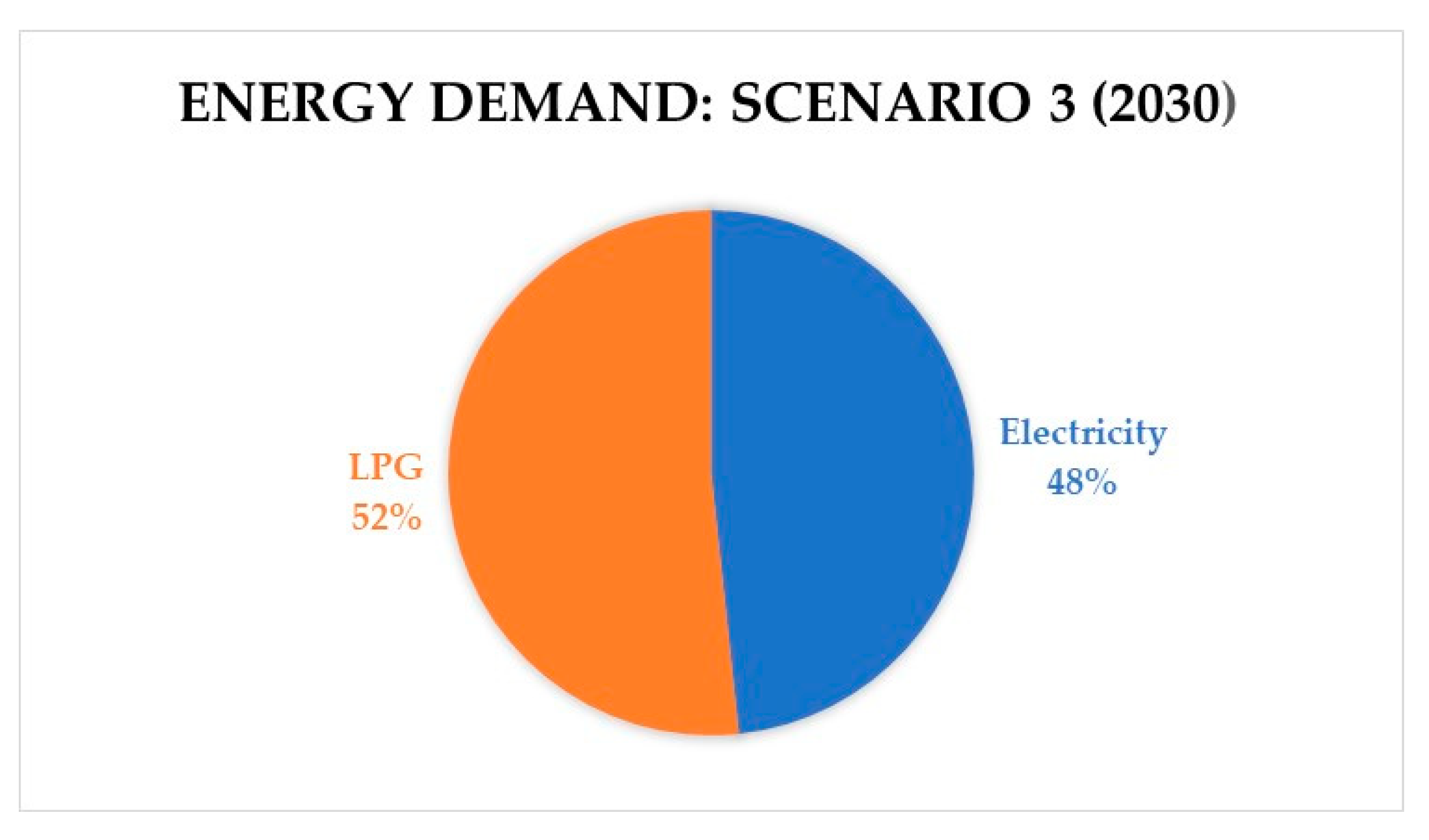
| Fuel | Base Year | Proportion |
|---|---|---|
| Electricity (kBOE) | 9.9145 | 8% |
| LPG (kBOE) | 108.3641 | 92% |
| EE | NG | GA | DI | FO | LPG | Solar | Heat | Total | |
|---|---|---|---|---|---|---|---|---|---|
| Production | 0.00 | 0.00 | 0.00 | 0.00 | 0.00 | 0.00 | 95.97 | 0.00 | 95.97 |
| Import | 281.29 | 59.47 | 984.85 | 789.35 | 218.49 | 313.58 | 0.00 | 0.00 | 2647.03 |
| Export | 0.00 | 0.00 | 0.00 | 0.00 | 0.00 | 0.00 | 0.00 | 0.00 | 0.00 |
| Total supply | 281.29 | 59.47 | 984.85 | 789.35 | 218.49 | 313.58 | 89.82 | 0.00 | 2709.40 |
| ST | 0.00 | 0.00 | 0.00 | 0.00 | 0.00 | 0.00 | −95.97 | 62.38 | 0.00 |
| Distribution | −19.69 | 0.00 | 0.00 | 0.00 | 0.00 | 0.00 | 0.00 | 0.00 | −19.69 |
| Total transformation | −19.69 | 0.00 | 0.00 | 0.00 | 0.00 | 0.00 | −95.97 | 62.38 | −19.69 |
| Residential | 101.55 | 0.00 | 0.00 | 0.00 | 0.00 | 181.51 | 0.00 | 62.38 | 345.44 |
| Industry | 61.89 | 59.47 | 0.00 | 127.33 | 216.55 | 98.68 | 0.00 | 0.00 | 563.92 |
| Transportation | 0.00 | 0.00 | 984.83 | 642.73 | 0.00 | 0.00 | 0.00 | 0.00 | 1627.56 |
| Commercial | 59.62 | 0.00 | 0.00 | 0.00 | 0.00 | 25.89 | 0.00 | 0.00 | 85.51 |
| Public lighting | 18.56 | 0.00 | 0.00 | 0.00 | 0.00 | 0.00 | 0.00 | 0.00 | 18.56 |
| Other | 19.98 | 0.00 | 0.02 | 19.29 | 1.93 | 7.49 | 0.00 | 0.00 | 48.72 |
| Total demand | 261.60 | 59.47 | 984.85 | 789.35 | 218.49 | 313.58 | 0.00 | 62.38 | 2689.71 |
| Scenario | IEp + IEs (MBOE) | ES (MBOE) | EA | EAn |
|---|---|---|---|---|
| Baseline | 2.736.75 | 2.736.75 | 1.00 | 0.00% |
| ES5 | 2647.03 | 2709.40 | 0.97 | 3.28% |
| System | Useful Life (Years) | Reference | Useful Life | Costs (USD kW Year) |
|---|---|---|---|---|
| Solar water heaters | 13 | [6] | 20 | 17.95 |
| 15 | [9] | |||
| 20 | [18] | |||
| 25 | [8] |
| Scenario | Inv. (USD/kW) | O&M (USD/kW) | r (%) | Useful Life (Years) | Power (MW) | Plant Factor (%) | Ce (USD/kWh) |
|---|---|---|---|---|---|---|---|
| E1 | 504.00 | 17.95 | 5 | 20 | 76.91 | 14.00 | 0.047 |
| Scenario | Ce (USD/kWh) | Ce (USD/BOE) | VAT (%) | Profit (%) | PE (USD/BOE) | Pen (%) |
|---|---|---|---|---|---|---|
| E1 | 0.047 | 77.60 | 0.00 | 0.00 | 77.60 | 82.67% |
| Energetic * | Price | Unit | Source | Pe (USD/BOE) |
|---|---|---|---|---|
| ES0 Elec | 0.0933 | USD/kWh | [48,49] | 150.71 |
| Es0 Residential LPG | 0.1066 | USD/kg | [49,50] | 13.10 |
| Is0 industrial LPG | 0.638 | USD/kg | [50] | 78.42 |
| ES0 Natural gas industry | 8.39 | USD/MMBtu | [29] | 46.29 |
| Is0 Residential gasoline | 1.30 | USD/gallon | [50] | 60.24 |
| ES0 Industrial gasoline | 1.49 | USD/gallon | [50] | 69.04 |
| ES0 Residential diesel | 0.90 | USD/gallon | [50] | 36.68 |
| ES0 Industrial diesel | 1.32 | USD/gallon | [50] | 52.58 |
| ES0 Fuel gas | 0.80 | USD/gallon | [50] | 32.19 |
| Scenario | ΣPej × Ej (M USD) | ΣEj (k BEP) | PME (USD/BEP) | PMEn (%) |
|---|---|---|---|---|
| ES0 | 150,846.74 | 2717.00 | 55.52 | 48.27% |
| ES5 | 154,407.44 | 2689.71 | 57.41 | 41.98% |
| Scenario | RE (kBOE) | ES * (kBOE) | UR | Urn (%) |
|---|---|---|---|---|
| ES0 | 0.00 | 2736.75 | 0.00 | 0.00% |
| ES1 | 62.38 | 2709.40 | 0.02 | 2.30% |
| Scenario | Ree (kBOE) | Ese (kBOE) | Ure | Uren (%) |
|---|---|---|---|---|
| Es0 | 0.00 | 282.13 | 0.00 | 0.00% |
| Es1 | 0.00 | 281.29 | 0.00 | 0.00% |
| Scenario | CEC (kT CO2) | ED (kBOE) | Pre (t CO2/BOE) | Pren (%) |
|---|---|---|---|---|
| Es0 | 987.61 | 2717.00 | 0.363 | 34.16% |
| Es1 | 949.93 | 2689.71 | 0.353 | 36.74% |
| System | CIM (People-Year/MW) | OM (Jobs/MW) | References | Ie (Total Jobs-Year/GWh) | |
|---|---|---|---|---|---|
| Solar water heaters | 8.40 | * | [51] | 0.34 | 0.52 |
| 22.40 | [52] | 0.91 | |||
| 7.40 | [53] | 0.30 | |||
| System | Ie (Total Jobs-Year/GWh) | Source | Ie (Total Jobs-Year/GWh) |
|---|---|---|---|
| Hydropower * | 0.05 | [51] | 0.05 |
| Fossil fuel electricity * | 0.11 | [54] | 0.11 |
| Fossil fuels ** | 0.05 | [51] | 0.07 |
| 0.09 | [54] |
| Scenario | Em (Jobs-Year) | Emn (%) |
|---|---|---|
| Es0 | 315.00 | 2.14% |
| Es5 | 356.94 | 8.13% |
| Denomination | Flat Plate Collectors | Evacuated Tube Collectors | Units |
|---|---|---|---|
| Energy demand | 9534 | 9534 | MJ |
| Solar coverage | 6674.9375 | 6674.9375 | MJ |
| Auxiliary coverage | 2860.6875 | 2860.6875 | MJ |
| Investment cost | 887.5 | 1425 | USD |
| 15 kg tank | 204.649 | 204.65 | kWh |
| 15 kg tank | 736.73 | 736.74 | MJ |
| Gas equivalent | 9.06 | 9.06 | Tanks |
| Subsidized tank cost | 3 | 3.00 | USD |
| Unsubsidized tank cost | 13.60 | 13.60 | USD |
| Total cost with subsidy | 27.18 | 27.18 | USD |
| Total cost without subsidy | 123.24 | 123.24 | USD |
| Amortization time with subsidy | 32.65 | 52.43 | years |
| Amortization time without subsidy | 7.20 | 11.56 | years |
Publisher’s Note: MDPI stays neutral with regard to jurisdictional claims in published maps and institutional affiliations. |
© 2022 by the authors. Licensee MDPI, Basel, Switzerland. This article is an open access article distributed under the terms and conditions of the Creative Commons Attribution (CC BY) license (https://creativecommons.org/licenses/by/4.0/).
Share and Cite
Barragán-Escandón, E.A.; Zalamea-León, E.; Calle-Sigüencia, J.; Terrados-Cepeda, J. Impact of Solar Thermal Energy on the Energy Matrix under Equatorial Andean Context. Energies 2022, 15, 5803. https://doi.org/10.3390/en15165803
Barragán-Escandón EA, Zalamea-León E, Calle-Sigüencia J, Terrados-Cepeda J. Impact of Solar Thermal Energy on the Energy Matrix under Equatorial Andean Context. Energies. 2022; 15(16):5803. https://doi.org/10.3390/en15165803
Chicago/Turabian StyleBarragán-Escandón, Edgar A., Esteban Zalamea-León, John Calle-Sigüencia, and Julio Terrados-Cepeda. 2022. "Impact of Solar Thermal Energy on the Energy Matrix under Equatorial Andean Context" Energies 15, no. 16: 5803. https://doi.org/10.3390/en15165803
APA StyleBarragán-Escandón, E. A., Zalamea-León, E., Calle-Sigüencia, J., & Terrados-Cepeda, J. (2022). Impact of Solar Thermal Energy on the Energy Matrix under Equatorial Andean Context. Energies, 15(16), 5803. https://doi.org/10.3390/en15165803