Article

Fault Identification and Fault Impact Analysis of The Vapor Compression Refrigeration Systems in Buildings: A System Reliability Approach

by
Mostafa Fadaeefath Abadi
*,
Mohammad Hosseini Rahdar
,
Fuzhan Nasiri
and
Fariborz Haghighat
Department of Building, Civil and Environmental Engineering (BCEE), Gina Cody School of Engineering and Computer Science, Concordia University, Montréal, QC H3G 1M8, Canada
*
Author to whom correspondence should be addressed.
Energies 2022, 15(16), 5774; https://doi.org/10.3390/en15165774
Submission received: 26 May 2022 / Revised: 27 July 2022 / Accepted: 29 July 2022 / Published: 9 August 2022

Abstract

:
The Vapor Compression Refrigeration System (VCRS) is one of the most critical systems in buildings typically used in Heating, Ventilation, and Air Conditioning (HVAC) systems in residential and industrial sections. Therefore, identifying their faults and evaluating their reliability are essential to ensure the required operations and performance in these systems. Various components and subsystems are included in the VCRS, which need to be analyzed for system reliability. This research’s objective is conducting a comprehensive system reliability analysis on the VCRS by focusing on fault identification and determining the fault impacts on these systems. A typical VCRS in an office building is selected for this research regarding this objective. The corresponding reliability data, including the probability distributions and parameters, are collected from references to perform the reliability evaluation on the components and subsystems of the VCRS. Then the optimum distribution parameters have been obtained in the next step as the main findings. Additionally, by applying optimization techniques, efforts have been taken to maximize the system’s reliability. Finally, a comparison between the primary and the optimized systems (with new distribution parameters) has been performed over their lifetime to illustrate the system’s improvement percentage.

1. Introduction

The vapor compression refrigeration cycle is an essential system that has been widely used in residential, commercial, and industrial sections, including refrigerators, refrigeration air conditioning, freezers, and air conditioning systems. Different types of refrigeration systems are used depending on the application. In the commercial sector, the multiplex direct expansion system is used for refrigeration systems in supermarkets. These systems typically use compressors and air-cooled condensers with axial blowers (working together) for the heat rejection process [1]. The main components or elements of these systems are compressors (C), evaporators (E), condensers and thermo-expansion valves (TEV). The evaporative condensers can be used in these systems, reducing condensing temperature and optimizing energy consumption [2]. Another feature of vapor compression is its ability to gain low evaporating temperatures. This action can be done while keeping a large cooling capacity per unit of power input to the system [3]. As mentioned, in addition to refrigerators, the VCRS is used in air conditioning systems which are available in several types having different refrigerants depending on their purposes [4]. According to research performed on a refrigeration system by Frenkel and Khvatskin, when a fault occurs in a machinery’s single unit or item, a harmful effect on the whole system will not be caused because of the system’s nature. However, the system’s cooling capacity will be reduced. However, when a component such as a compressor or the axial condenser blower fails, both partial system failure and complete system failure can occur. The components and subsystems of the refrigeration systems have arbitrary finite-state numbers, which means that due to various performance rates, the system may have different corresponding states. Hence, the refrigeration system is a Multi-State System (MSS). MSS models have been analysed and studied by researchers [2,5].
Since the components and subsystems in refrigeration systems have arbitrary finite-state numbers and could vary from perfect functioning to complete failure, the whole system is considered a multi-state one [1]. In these types of systems, the availability percentage of each unit has an impact on the whole system’s performance rate. Thus, having different numbers of the available units leads to various levels of task performance [2].
The reliability and optimization analysis and studies require mathematical formulations for the vapor compression refrigeration cycle. The term reliability has its origin in the failure analysis of electronic equipment for military use during the 1950s in the United States. Based on the literature, the system or product’s reliability is defined as the probability of performing the intended function for that system or product during a specific time horizon. This performance should be in normal operating conditions [6,7].
This research also applies the Failure Mode and Effects Analysis (FMEA) to identify different failure modes of the VCRS and their effects on the whole system. FMEA is used along with Criticality Analysis (CA) by researchers, highlighting the single-point failures requiring corrective action. FMEA can be applied to provide a ranking for the Failure Modes (FMs) of products and components, from the ones presenting the highest risk to those that present the lowest risk for the system [8]. FMEA also assists the development of test methods and enhances the troubleshooting techniques. Therefore, a foundation for qualitative reliability, maintainability, safety, and logistics analyses can be provided by applying the combination of FMEA and CA, known as FMECA [9].
A cooling system can be elaborated as a heat engine working in reverse, technically referred to as a reverse Carnot engine. In other words, it is the transfer of energy from a cold reservoir to a hot one. In the primary form of vapor refrigeration compression system, there are four major components: evaporator, compressor, condenser, and expansion valve. External energy (power) is supplied to the compressor, and heat is added to the system in the evaporator, whereas in the condenser, heat rejection occurs from the system. Heat rejection and heat addition are dissimilar to different refrigerants, which cause a change in energy efficiency for the systems. Exergy losses in various components of the system are not the same. The Schematic diagram of a typical vapor compression refrigeration cycle is shown in Figure 1, including its main components (evaporator, compressor, condenser and expansion valve). To take the heat from the external environment, the evaporator is used. The mechanical compressor, which consumes a considerable amount of energy, performs the suction process of evaporated vapors to compress and expel them at a higher pressure and temperature. The vapor refrigerant condenses in the condenser by transferring heat to the outdoor environment. Finally, through the expansion valve, the liquid refrigerant returns to the evaporator having a lower pressure for the cycle’s repetition [10].
Various research works and studies have been performed to evaluate different types of refrigeration systems. This section presents the vital relevant publications and research works. According to the recent literature, energy analysis and reliability analysis were mainly studied to evaluate such a system’s performance. The authors have thoroughly reviewed recent and relevant publications and presented them here.
For a supermarket refrigeration system, the reliability analysis and calculation have been performed by applying the combined stochastic process and universal generating function methods. Reliability measures for different performance levels are considered for the system’s structure in the decision-making process, and the availability, output performance and performance deficiency are achieved [1].
Concerning FMEA, various studies suggest different grouping and classifications of FMs for a system. To obtain the weights of risk factors, a consensus-based model is proposed within the FMEA framework. The objective of the research conducted by Hengjie Zhang et al. [8] was to classify the FMs according to a possibilistic fuzzy approach using linguistic information collected. In addition, they also presented a consensus rule-based optimization approach to minimize the adjustment distance in the consensus-reaching process. This minimization approach assists FMEA members in improving their consensus level. This optimization aims to reach the predefined consensus level among all FMEA members. Finally, the consensual FM risk classes were achieved [8]. A case study was implemented into an active Scanned Proton Beam (SPB) which is used in radiation therapy. The results of their research present the benefits of applying a Possibilistic Hesitant Fuzzy Linguistic Term Sets (PHFLTSs) approach. Since the FMEA members express their uncertain assessments, the PHFLTS has convenience and flexibility for handling hesitancy and uncertainty in practical contexts [8].
Another study presented an FMEA model based on Personalized Individual Semantics (PIS) [12]. By applying PIS along with the Linguistic Distribution Assessment Matrices (LDAMs), they used feedback and opinions collected from different FMEA experts to define the failure modes and risk factors. They proposed an incomplete Additive Preference Relations (APRs) which was used for incorporating the experts’ opinions about FMs. In addition, a two-stage optimization method is presented and applied. In first stage, they obtained the complete APRs and identified the PISs. In the second stage, a minimum-based optimization model has been used for consistency improvement which generates a complete APR with an acceptable consistency level. Another optimization model was formulated for minimizing the deviation between the APR and the numerical assessment matrix which is obtained from the corresponding LDAM. Finally, the researchers have ranked the FMs according to their corresponding risk factors. By implementing a case study and performing a detailed comparison analysis, the authors tested the validity of their proposed PIS-based linguistic FMEA model. The results of their study assist risk managers in identifying critical FMs to improve the system’s reliability and safety [12]. Another study used a Comparative Linguistic Expression Preference Relations (CLEPRs) tool for PISs assessment. This method is helpful in representing uncertain opinions of decision makers in Group Decision Making (GDM). The optimization model formulated and used by the authors assists in assessing individual semantics in CLEPRs and it is used to obtain PNSs of linguistic terms associated with FMEA members [13].
For Heating, Ventilation, and Air Conditioning (HVAC) systems in buildings, a data-driven fault detection and diagnosis (FDD) model has been proposed and applied in research work. This model is implemented for the Air Handling Units (AHUs) to enable reliable maintenance by considering undefined states. Based on the study’s results, their model could identify undefined and defined data with high performance. Therefore, the results of their research reached the objective of facilitating the maintenance management of AHUs in HVAC systems [14]. Scholars have also studied the large-scale industrial vapor-compression refrigeration systems to conduct an experimental dynamic performance analysis. This refrigeration system was a conventional industrial type included in a discrete cooling system, which was a cold storage facility warehouse. The energy, exergy, and exergoeconomic aspects were obtained by implementing a real-time data monitoring system for achieving future energy planning. According to the study’s results, future work towards energy management and further profit-making can be done [15].
The exergy analysis can be applied to different VCRSs based on their applications. Hence, various potential research topics are discovered by scholars. They have reviewed studies in various countries or societies in this field to highlight the importance of exergy analysis in VCRSs. Based on the findings, exergy depends on evaporating temperature, condensing temperature, sub-cooling and compressor pressure and the environmental temperature [4].
Another critical literature review has been performed for compact and miniature mechanical VCRSs regarding their fundamentals, design, and application aspects [3]. Their publication has highlighted the thermodynamic and thermal factors for the cooling cycle. The researchers have also reviewed recent advancements of the cooling cycle components such as the compressor, heat exchangers and the expansion device. They have also presented the main issues related to different cycle designs and recent works on new technologies. Various VCRS electronics and personal cooling devices have been compared in their comprehensive review concerning technical information and application [3].
Regarding maintenance management, research works have been performed for processing plants. To evaluate the technical and economic feasibility of a condition-based maintenance task, an HVAC system in a pharmaceutical laboratory was selected as the case study. The corrective, time-based and condition-based maintenance strategies were chosen and investigated to obtain the most efficient economic strategy. Their research has also implemented a reliability continuous monitoring system to evaluate its cost-effectiveness [16]. The scholars have provided valuable results for facility service and process plant managers.
Moreover, researchers have recently focused on the environmental impacts of widely used refrigerants applied in air conditioning and refrigeration systems regarding international agreements. The development of such refrigerants has also been considered and studied. Considering the leakage of these systems, equivalent CO2 emission value has been calculated and analyzed based on the leakage rate and initial charge number of different refrigerants. Different air conditioning and refrigeration systems have been included in this research in terms of their types and sizes [10].
Identifying failures for VCRS is of particular importance due to the critical role of this system in HVAC systems. In this sense, the main motivation for this research is to enhance the reliability and performance of VCRS improving the HVAC system. Hence, the primary objective of this research is to evaluate the reliability of components as well as whole system to identify pathways to reduce the failure and increase the whole system’s reliability. The system considered for this study is used to provide and supply cooling load for an office building. The analysis is based on a failure database, which presents the failure modes and time-to-failure reports in reciprocating and retaliating systems provided by maintenance management companies and derived from the literature and relevant studies.
In this paper, some basic information about the concept of the vapor compression system is given, and the system’s operations are explained.
In the first part of this work, by collecting data and using relevant references, a reliability analysis was performed on this system to determine the relevant parameters for each random variable (a component in the system). Then, the corresponding reliability parameters and functions are calculated. The second part represents the Reliability Block Diagram (RBD) for the VCRS, which defines and illustrates the components, units, and subsystems established in the whole system. Then, the reliability parameters such as the Mean Time to Failure (MTTF), median value, and the standard deviation, calculated for the whole system are obtained. Using these data, an optimization model based on the Genetic Algorithm (GA) method has been created by the MATLAB software to optimize the system’s reliability. Finally, the impact of modifying the system’s configuration on its reliability improvement is highlighted, and a comparison between the basic system and the optimized system in terms of system reliability is presented.

2. System and Methodology

2.1. System’s Components and Configuation

The system selected for this research is a vapor compression refrigeration system. This system is employed to provide a 1000 kW cooling load for an office building. Three identical units (Unit A), each having a cooling load of 500 kW, are considered for providing demanded load as a 2-of-3 reliability system. A control system monitors the working situation of these three units. It is placed before these units. Each cooling unit (Unit A) consists of a cooling tower, a condenser, a compressor, an expansion valve, an evaporator, water circulating pump, piping, a set of three parallel air filters and eventually, a set of two AHUs. Additionally, a simplified assumption for perfect switching in the case of standby units has been considered in this system (Figure 2). It should also be noted that based on the assumptions in this research and in terms of reliability analysis, the air filters are considered separate components and are placed before the AHUs in the system’s configuration.
The system working environment is realized critical from the aspect of dust particles and considering this fact would justify placing three air filters in a parallel situation.
In addition, AHUs are typically constructed onsite and work with several components which are connected to the building. They usually include fans, a cooling coil, a heating coil, coil control valves, various dampers, and sensors. The equipment components and physical assets of AHUs could have different specifications based on the site’s features. Therefore, defining a standard system for AHUs is not always possible. Additionally, it is difficult to notice malfunctions and deterioration of AHUs. Due to not preventing these issues at the right moment, maintenance costs and energy consumption will be increased in the future. Depending on different seasons, various faults could occur in AHUs, including the damper leak, the damper stuck, the cooling coil valve stuck and the reduced capacity of the heating coil [14]. Hence, the AHU is considered a critical part of the system, which is statistically a vulnerable component.
Therefore, to avoid its highly negative influence on the system’s reliability, the authors considered one standby unit for it while it does have an inconsiderable cost compared to the system’s total cost. The system would be evaluated in terms of all reliability aspects and the effect of having redundancy components (in parallel, standby and r-of-n).

2.2. System’s Reliability Data

The system’s configuration for this research has been designed to supply the required load (1000 kW) which has three 500 kW units (each called unit A) in the form of 2 out of 3 (r-out-of-n configuration). According to reliability engineering’s concepts, this particular configuration, also known as the k-out-of-n configuration, is represented by a system operative when a minimum k number of components (elements) out of a total of n components (elements) are available for normal operation in a system. It is also defined as k-out-of-n redundancy with k ≤ n [17]. Thus, based on the assumption considered for this research, at least 2 of all 3 units should successfully operate simultaneously.
Depending on each component’s failure time distribution, reliability parameters for each have been derived from the literature, relevant references, and reliability handbooks. Distributions have been selected from four different continuous distribution functions, including Exponential, Rayleigh, Weibull and Uniform (Rectangular).
Based on each distribution’s parameters, the statistical parameters of reliability (mean value, median value, and standard deviation), as well as the reliability of each component, could be calculated and obtained. Then, a comprehensive and step-by-step assessment of the system will be done. To better illustrate the impacts of each configuration (e.g., r-out-of-n, parallel and standby), a graphical representation is provided.

2.2.1. Probability Distributions Applied for the Components of the System

Exponential Distribution

The exponential, or strictly the negative exponential, distribution is probably the most widely known and used distribution in the reliability evaluation of systems due to its simplicity [17]. One positive scale parameter which is λ is defined as the failure rate that shows the number of failures in a specific time horizon [17]. This vital factor is applicable for the exponential distribution as the hazard rate, which is constant. This is essentially the exact requirement as that of the Poisson distribution, and it can be argued that the negative exponential distribution is only a particular case of the Poisson distribution, i.e., when considering the probability of the first failure. In practice, the negative exponential distribution has a much wider degree of significance than just that of the first failure and is extensively used in the analysis of repairable systems in which the components cycle between operating or up states and failure or down states.
It should also be noted that the hazard rate is not absolutely constant. However, most stationary components express a nearly constant failure rate behavior. Considering that there is a very limited amount of information about failure distribution parameters for many of the investigated components in reliability engineering references and handbooks (such as Offshore & Onshore Reliability Data Handbook), exponential failure distributions (with constant failure rates) are used in this study [18].
The probability of a component surviving for a time t if the hazard rate is constant is defined as the survivor function, which is shown below:
R(t) = e−λt,
Therefore, the failure density function is:
f(t) = −dR(t)/dt = λ × e−λt,
In addition, the cumulative failure distribution, Q(t) and the survivor function, R(t), are as follows:
Q ( t ) = 0 t λ × e λ t = 1 e λ t ,
R ( t ) = t λ × e λ t = e λ t
The hazard (failure) rate, which is a conditioned probability for an object that breaks down (fails) in a specific time interval [17] is calculated by dividing the failure density function by the survivor function as follows:
λ(t) = f(t)/R(t)
It is worth noting that in addition to a hazard rate, which is the probability of failure occurrence in the immediate future, the reverse hazard rate had been considered and calculated in this research. The reverse hazard rate, which is the dual to the hazard function, represents the probability of an immediate past failure for a component which has already been failed at time t. This function has been considered and used in different research works [19] and can be obtained as follows:
Reversed hazard function = (λ(t) × R(t))/Q(t)
The reversed hazard function has been evaluated and applied for different applications by researchers, such as performing the reversed hazard rate ordering. For instance, formulating the uncertain past lifetime and calculating the past entropy (the residual entropy referring to the past time) can be done by using this function [20,21].

Weibull Distribution

This continuous random variable distribution is named after W. Weibull, a Swedish mechanical engineering professor. The distribution can be used to represent many different physical phenomena. Depending upon the values of the parameters in its reliability functions, it can be shaped to represent many distributions as well as shaped to fit sets of experimental data that cannot be characterized as a particular distribution other than as a Weibull distribution with specific shaping parameters. The engineering judgment and data are used with Weibayes estimates, the failure mode’s estimation. Weibull’s distribution is formulated by having the failure mode characterized with a slope (b) and considering the relating age and probability of failure. This approach is to create understandable and practical datasets [22].
For this reason, the Weibull distribution has a crucial role to play in the statistical analysis of experimental data. A particular type of graph paper known as Weibull probability paper is readily available, on which the experimental data can be plotted. This paper is so constructed that the Weibull parameters can be easily deduced from the experimental plots. The great adaptability of the Weibull distribution can be seen by considering the pertinent functions.
The failure density function of the Weibull distribution is defined as:
f(t) = [(β × tβ−1)/(αβ)] × exp[−(t/α)β],
where α and β are distribution shape and scale parameters, respectively.
The survivor function is:
R ( t ) = t f t dt = exp [ ( t / α ) β ] ,
The cumulative failure distribution is:
Q(t) = 1 − R(t) = 1 − exp[−(t/α)β],
The hazard rate is:
λ(t) = f(t)/R(t) = (β × tβ−1)/(αβ),
The mean time to failure is:
MTTF = α × Γ × [(1/β)+1],
where Γ is the gamma function defined as:
Γ ( γ ) = 0 t γ 1 × e t dt ,
Which, for integer values of γ, reduces to:
(γ) = (γ − 1)!

Rayleigh Distribution

This continuous random variable distribution, often used in the theory of sound and in reliability studies, is named after John Rayleigh (1842–1919) [23]. Although the Rayleigh distribution was introduced as a special case of the Weibull distribution, it is considered as an important distribution in its own right. It is not only applied in reliability problems but also in noise problems associated with communications systems. Unlike the Weibull and gamma distributions, which are characterized by two parameters, the Rayleigh distribution is a single parameter distribution like the exponential distribution.
It is worth bearing in mind that although the Rayleigh distribution has an increasing failure rate, for those with shape factors lower than 0.5, it has a decreasing failure rate at the beginning. After a time, the failure rate increases again (U-shape hazard function). This behavior is reasonable since most electric systems have either a failure at the beginning or in the long-term operation.
Rayleigh’s probability density function is expressed by:
f(t) = 2t/α2 × exp[−t22],
This equation indicates that the single parameter is α. A more general expression for the failure density function is:
f(t) = kt × exp[−kt2/2],
In which k is the single parameter and which is equivalent to the particular case of the Weibull distribution (β = 2), when k = 2/α𝟐.
The survivor function is:
R(t) = exp[−kt2/2],
Moreover, the cumulative failure distribution is:
Q(t) = 1 − R(t) = 1 − exp[−kt2/2],
The hazard rate is:
λ(t) = k × t,
Finally, the Mean Time To Failure (MTTF) is:
π / 2 × k

Uniform Distribution

As the simplest distribution, it is sometimes known as a rectangular distribution and is considered a particular case of the geometric probabilities introduced and discussed in references [24]. This distribution has constant probability and a random X variable, which is restricted to a finite interval [a, b]. Thus, the random variable is uniformly distributed in the interval [24]. The failure density and survivor functions for the uniform or rectangular distribution are below.
f(t) = 1/(b − a),
R(t) = (b − t)/(b − a)
The following calculations could be obtained by having the definitions of expectation and variance. As expected, the uniform distribution does not have complex equations and calculations, and according to the basic definition of expectation, the following equations are achieved:
λ(t) = 1/(b − t),
MTTF = (a + b)/2,
𝜎 = (b − a)2/12

3. Results

In this section, a concise and precise description of the calculations and results according to the case study are presented, and interpretations of the conclusions of this research are also drawn.
The first part of this section provides calculations for statistical reliability parameters of each component, the subsystems, and the whole system. Then, in the second part, the reliability functions of the components, subsystems and the whole system are calculated and obtained. Finally, in the third part, details regarding optimizing the system’s reliability are shown. The optimized values for each component and the comparison between the original system and the optimum one are also included in the third part of this section.

3.1. Statistical Parameters for Each Component

The statistical parameters of system components, including MTTF, the median time to failure and standard deviation, are calculated by taking the failure density function parameters into account and following the distribution formulas.

3.1.1. Reliability Function

As explained previously, the distribution parameters were obtained from different references and indexed in Table 1. Then, failure and reliability function depending on the time for each component would be achieved, which are listed in Table 2.

3.1.2. Mean Time to Failure (MTTF)

This parameter is the length of time a device or other product is expected to last in operation. MTTF is one of many ways to evaluate the reliability of pieces of hardware or other technology.
In some references, a Mean Time Between Failure (MTBF) is calculated. It is computed as the average time between failure occurrences of components, which is applicable to all types of systems. On the contrary, MTTF is generally used for replaceable or non-repairable components or devices in a system and is used in calculation of components failure rates [25,26].
MTTF represents how long a product can reasonably be expected to perform in the field considering specific testing. However, it should be noted that MTTF metrics provided by companies for specific products or components may not have been obtained by running one unit continuously until failure. This metric could be alternatively achieved by running many units, even thousands of units, for a specific number of hours [27]. The MTTF could be calculated by taking the integration of the reliability function between 0 and infinity. These calculations have been conducted for each component in the case study’s system and are listed in Table 3.
Another important criterion which is considered in the reliability analysis is the Mean Residual Lifetime (MRL) of a component or asset. This parameter is calculated in different studies to find the expected lifetime of a component after its current age. It is usually studied to obtain an optimal burn-in time for a component or asset [28]. MRL is calculated depending on the component’s failure distribution. In the exponential distribution, due to the memory-less property, MRL is constant and is equal to the MTTF which is 1/λ. Hence, since it is assumed that most of the components used in this research follow an exponential failure distribution, the MRL has not been calculated separately.

3.1.3. Median Time to Failure

This parameter is obtained and used to evaluate the time of reaching the reliability or unreliability of the component to 50%. The median time of components for the case study’s system are indexed below in Table 4.

3.1.4. Standard Deviation

The Standard Deviation (SD), also represented by the Greek letter sigma σ or the Latin letter s), is a statistical measure for quantifying the variation’s amount or dispersion of a set of data values. For measuring the data’s dispersion in a given dataset about the mean, SD has been widely used in the literature and by researchers [29].
A low standard deviation is defined when the data points tend to be close to the mean (also called the expected value) of the set. On the other hand, we have a high standard deviation when the data points are spread out over a broader range of values [30]. In this research, the SD has been calculated for all the components, and the results are presented in Table 5.

3.2. Reliability Parameters & Functions for the Subsystems and the Whole System

3.2.1. Reliability of the Components

In this section, according to the reliability equations previously shown for each component in Table 2, the reliability of each component has been calculated for three different times (3000, 20,000 and 35,000 h) and is illustrated below in Table 6.
In addition, the mean and median time to failure parameters of the air filter and the AHU, which are considered a subsystem in unit A, are presented in Table 7.
For more comprehensive evaluation and for understanding the change of reliability function for components during their lifetime, the graphical method is more appropriate. Thus, the reliability curve of some of the most critical components is shown in Figure 3.
It could be seen in Figure 3 that after 5000 h from the beginning of the unit’s operation, the reliability of some components, such as the cooling tower and compressor will dramatically decrease. On the other hand, according to the same diagram, redundant parts are available in several sections of the system.
The impact of using redundant components for the air filter and the AHU will now be evaluated. First, having three air filters in the parallel configuration instead of one has been assumed and evaluated. Figure 4 illustrates how the system’s reliability differs while adding two additional filters before the AHU.
Reliability of one air filter having two additional filters compared to an induvial one after 20,000 and 35,000 h of operation will be 21% and 39% higher, respectively.
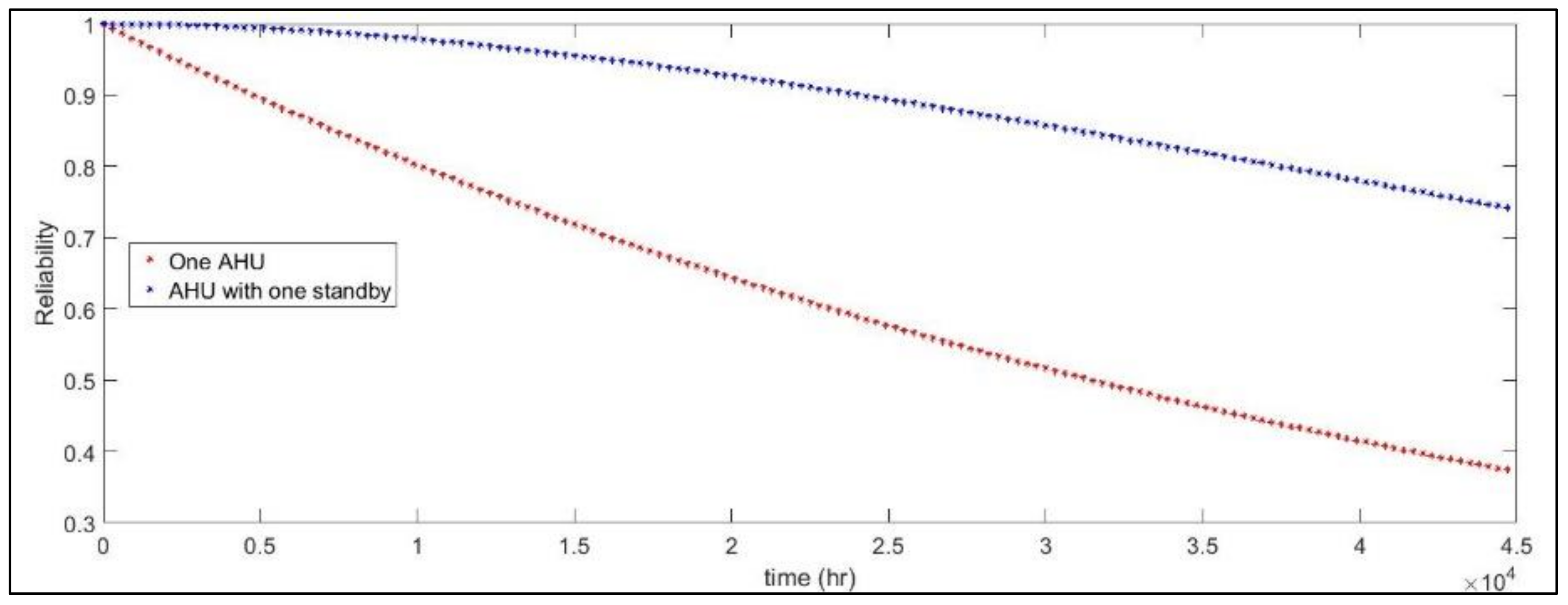
Regarding the AHU, an extra unit is considered a standby state with perfect switching. Figure 5 shows the variation trend in the case of an individual AHU compared to having an additional standby unit.
Again, adding an AHU in the standby state will increase the reliability compared to the situation with only one stand-alone AHU. The reliability increase is 45% and 77% after 20,000 and 35,000 h of operation, respectively.

3.2.2. Reliability of the Subsystems and Whole System

Unit A consists of compressor, evaporator, condenser, pump, piping, cooling tower, expansion valve, AHU (in standby mode) and air filter (with parallel configuration) which makes the main subsystem of the whole system. Based on the research’s assumption, unit A provides 500 kW and to supply 1000 kW required cooling load, three units the same as unit A are used to supply this demanded load. Taking the reliability of each component into consideration, the equivalent reliability of unit A would be obtained as below:
RUnit A = RCooling-Tower × RCondenser × RCompressor × RExpansion-valve × REvaporator × RPump × RPiping × RFilter × RAHU
R Un it A = e 2.84 + 2.3 + 2.3 + 12.058 + 22 + 0.02 × 10 6 t × 3 e 10 × 10 6 t 3 e 20 × 10 6 t + e 30 × 10 6 t × e t 29856 1.87 × 1 + 22 × 10 6 × t × 130000 t 128000
R Unit A = 3 e 51.518 t × 10 6 t 3 e 61.518 t × 10 6 t + e 71.518 t × 10 6 t 1 + 22 × 10 6 × t × e t 29856 1.87 × 130000 t 128000
The reliability curve of unit A is shown in Figure 6A–D. This curve trend comes with an exponential curve due to multiplying several exponential equations and a linear equation. To assess the most effective components in reducing the reliability of unit A, a parametric study on each component was carried out in this research, and the results of this study are provided in this section.
For this purpose, the time of 20,000 h is fixed, and a range of variation is determined for the component’s reliability. Hence, the influence of the component’s reliability changes on the reliability of unit A could be observed and evaluated. The reliability of unit A at 20,000 h before performing the parametric study was 0.2005.
Four critical components of unit A have been selected in this study and their failure parameters (hazard rates for the evaporator, AHU, cooling tower and α for the compressor) varied in the range of 20% higher and 20% lower of the primary value. The time of 20,000 h is fixed and only one failure parameter of a particular component is considered as the variable. Then, the reliability of unit A is calculated based on the variation of that component’s reliability.
In fact, this sensitivity analysis determines how the failure parameter can affect the component’s reliability and, in sequence, illustrates the influence of the reliability of that component on the reliability of unit A. In the case of the compressor, it is observed that the increase in α has a lower effect on the compressor’s reliability than its reduction. In general, a 40% fluctuation of α can change unit A reliability by 7%.
For the AHU, the impact is not as significant as the compressor, while 40% fluctuation of the compressor’s hazard rate can influence its reliability by 5% and will make a 1.1% change for unit A’s reliability. Evaporator and condenser with the same failure rates have a lower impact on unit A’s reliability since a 40% change in their hazard rates will only create a 1.7% variation in their reliability and a 0.4% change in unit A. Finally, 40% fluctuation of the cooling tower’s hazard rate will affect its reliability and unit A’s reliability by 13% and 4.5%, respectively.
Now, according to the equation below, we consider the whole system with three units of A in 2-out-of-3 configuration having a control system in series.
R sys = ( 3 × R A 2 × Q A + R A 3 ) × e k × t 2 2
It is expected that the whole system would experience higher reliability compared to unit A’s reliability because of the 2-out-of-3 arrangement. However, since the reliability of the control system shall be in the series state with other parts of the system, it could compromise the whole system reliability.
In Figure 7, the diagram compares the reliability profile of the complete system with unit A as well as the system without a redundant unit. For example, in time of 10,000 h, the reliability of unit A, complete system and system without redundancy is 51%, 46%, and 23%, respectively.

3.2.3. MTTF of the Subsystems and the Whole System

To calculate the mean time to failure of unit A, integration unit A’s reliability in the range of 0 to infinity is inevitable. As seen in the equation below, the term under integration is too much complicated and it is solved by numerical methods.
MTTF unitA = 0 RA dt = 0 3 e 51.518 t × 10 6 t 3 e 61.518 t × 10 6 t + e 71.518 t × 10 6 t × 1 + 22 × 10 6 × t × e t 29856 1.87 × 130,000 t 128,000 dt = 12,529 h
The MTTF of the complete system is also calculated with the same process as unit A although the term under integration becomes more complicated than the preceding one.
R sys = ( 3 × R A 2 × 1 R A + R A 3 ) × e k × t 2 2
MTTF sys = 0 R sys dt = 10,312 h

3.2.4. Median Time of the Subsystems and the Whole System

Obtaining the median time for unit A (the time of reaching reliability to 50%) due to the complex equation form should be solved by trial and error methods which could be done in MATLAB software. Therefore, this software has been applied in this research for the calculation.
R ( T 50 ) = 3 e 51.818 t × 10 6 t 3 e 61.818 t × 10 6 t + e 71.818 t × 10 6 t 1 + 22 × 10 6 × t × 3 e t 29,856 1.87 = 0.5
Thus, solving the above equation means that the median time for unit A is 10,323 h. For the complete system, the calculation is conducted similarly by substituting the reliability by 0.5 in the whole system’s reliability function and finding the time.
R sys ( T 50 ) = ( 3 × R A 2 × 1 R A + R A 3 ) × e k × t 2 2
Hence, the complete system’s median time is 9401 h.

3.3. Optimization

Generally, the optimization term conducts independent variables to a certain point to maximize or minimize dependent variables. Optimization implementation always requires making an algorithm code (such as a genetic algorithm or particle swarm optimization algorithm, etc.) in a programming language (such as FORTRAN, C+, MATLAB, etc.). There would often be particular constraints in each optimization process to limit independent variables. Otherwise, they always tend to go far towards positive or negative infinity.
Before starting the optimization procedure for the current problem, it can be predicted that for maximizing the total system’s reliability, the failure rate of components should lessen. However, we do not have a clear idea in the case of other distributions parameters like Weibull and Rayleigh. With this context, optimization of an independent variable is selected, which considers the distribution parameters to maximize the system’s probability.
As a searching area for the independent variables in this research, we considered 20% higher and 20% lower than their specific value as the threshold in order to perform an algorithm search for the best value among this range while the reliability reaches a peak. A Genetic Algorithm (GA) was coded to carry out this task for this research. Compared to single solution algorithms and methodologies, GA has the ability to process global searching for a population of solutions. It was introduced as a valid optimization method that can adapt and replicate the natural biological evolution process. The process produces fitter solutions which can lead towards obtaining an optimal solution [31]. Based on a primary guess for the variable in the given range, a couple of outputs from the fitness function are produced.
In the next step, a crossover and mutation process is applied to a certain percentage of variables, and the new population from the fitness function would be created. The new population is merged with previous ones. This cycle would continue to a certain number of trials or generations or can be terminated after a specified computation time to achieve the optimal solution [31]. Finally, the available population would be sorted, and the highest is found based on the goal, which is a maximization of the problem.
In Table 8, the optimum variable value for each distribution parameter is shown. Figure 8 compares the basic system and the optimized one with new distribution parameters over their lifetime.
An increase in reliability percentage between the basic system and the optimized one is given in Table 9.
Eventually, the MTTF and median time for the optimized system were calculated, and 29% and 32% increases were observed in results compared to the basic system.
MTTF (optimized system) = 13,344 h
Median Time (optimized system) = 12,400 h

4. Discussion

This section discusses the results and provides their interpretation from the perspective of previous studies and of the working hypotheses. The findings of this research and their implications are also included.
In the process of calculating the reliability of some components, because of some limitations in the working conditions and the high cost of such devices, the designers of this system did not consider any redundant devices for these components. This issue may be one of several drawbacks for keep system reliability high over a long period. However, some methods, such as periodical maintenance, could cover this weak point.
Based on the reliability results, applying two additional air filters (three filters in total) for this system could increase the reliability at more operating time. Moreover, adding an extra AHU as a standby state, has the same impact and could improve the reliability significantly compared to the situation having only one AHU. Additionally, some components have shown more criticality in terms of the system’s reliability.
This study determined that improving the reliability of some components, such as the compressor and the cooling tower could improve the reliability of the subsystem (unit A). In contrast, some other components, such as the evaporator and the air handling unit, had little effect on the subsystem reliability.
According to the GA optimization model and regarding the comparison results between the basic and optimized systems, the data illustrate that during the useful lifetime of the system, a significant improvement could happen if there is a chance of modification in the distribution parameters.

5. Conclusions

In this study, a VCRS was selected to perform a reliability analysis to investigate the reliability of the system and explore the ways to improve it. A Reliability Block Diagram (RBD) method was deployed to define the components, units, and subsystems for this system. A parametric study was conducted in order to investigate the effect of the component’s reliability on the whole system’s reliability. Finally, a single-objective Genetic Algorithm (GA) was used to optimize the total system reliability changing some potential components of the proposed system. Results reveal that the key components to this system’s reliability are rotary components such as compressor, fans, and pumps as well as electrical ones such as the control system. Most of the faults have been recorded within the aforementioned components by which they are the costliest parts of the VCRS. The compressors and cooling towers experience the most severe reduction in reliability over the course of time, while piping and heat exchanger are the most reliable parts.
From this research, it was concluded that using components with partial loads together improves the system reliability compared to a single component operating at full load. Optimization results show that investment in choosing the high-quality rotary components through the system, which technically means a better reliability curve, can enhance system reliability by nearly 10% in a 5000-h operation of the system, which is a significant improvement.
Despite efforts that have been made in this study, there are many gaps in this area. One recommended study for the future is considering the economic aspects of this system and its relevant components. Having capital and maintenance costs of components, a multi-objective optimization model can be taken into account for a comprehensive reliability-maintenance analysis; a preventive maintenance plan can be proposed for a better reliability-availability of the system.

Author Contributions

Conceptualization, M.H.R.; Formal analysis, M.H.R.; Investigation, M.H.R.; Methodology, M.H.R.; Resources, M.F.A. and M.H.R.; Software, M.H.R.; Supervision, F.N. and F.H.; Validation, M.H.R.; Visualization, M.H.R.; Writing—original draft, M.F.A. and M.H.R.; Writing—review & editing, M.F.A., F.N. and F.H. All authors have read and agreed to the published version of the manuscript.

Funding

This research received no external funding.

Institutional Review Board Statement

Not applicable.

Informed Consent Statement

Not applicable.

Data Availability Statement

The study did not report any data.

Conflicts of Interest

The authors declare no conflict of interest.

Nomenclature

VCRSVapor Compression Refrigeration System
HVACHeating, Ventilation, and Air Conditioning
FMEAFailure Mode and Effects Analysis
FMFailure Mode
CACriticality Analysis
RBDReliability Block Diagram
AHUAir Handling Unit
GAGenetic Algorithm
R(t)Survivor function, system or component reliability. A system’s (or component’s) probability for performing its specified mission satisfactorily in a specific time horizon operating based on specified conditions [29].
Q(t)Cumulative failure distribution is used to calculate the failure probability based on time (or another random variable) [32].
f(t)The derivative of Q(t) gives a function equivalent to the probability density function, and it is known as the failure density function [32].
λFailure (Hazard) rate shows the number of failures in a specific time horizon.
MTTFMean Time To Failure, which is the length of time when a replaceable or non-repairable component is expected to last in operation.
MTBFMean Time Between Failure, which is the computed average time between failure occurrences for repairable components.
MRLMean Residual Lifetime
σStandard Deviation (SD)
αThe shape parameter for Weibull and Gamma distributions. Changes to this parameter can be made to fit or approximate a wide range of experimental data.
βThe scale parameter for Weibull and Gamma distributions can be modified to fit or approximate a wide range of experimental data [32].
ΓThe Gamma function is used for Weibull and Gamma distributions.
γInteger values in the Gamma distribution.
a, bThe range of the random variables between a and b for the Rectangular (or Uniform) distribution [32].

References

  1. Frenkel, I.; Khvatskin, L. Reliability Decisions for Supermarket Refrigeration System by using Combined Stochastic Process and Universal Generating Function Method: Case Study. In Recent Advances in System Reliability; Springer: Berlin/Heidelberg, Germany, 2012; pp. 97–112. [Google Scholar]
  2. Lisnianski, A.; Frenkel, I.; Ding, Y. Multi-State System Reliability Analysis and Optimization for Engineers and Industrial Managers; Springer Science & Business Media: London, UK, 2010. [Google Scholar]
  3. Barbosa, J.R., Jr.; Ribeiro, G.B.; de Oliveira, P.A. A state-of-the-art review of compact vapor compression refrigeration systems and their applications. Heat Transf. Eng. 2012, 33, 356–374. [Google Scholar] [CrossRef]
  4. Ahamed, J.U.; Saidur, R.; Masjuki, H.H. A review on exergy analysis of vapor compression refrigeration system. Renew. Sustain. Energy Rev. 2011, 15, 1593–1600. [Google Scholar] [CrossRef]
  5. Lisnianski, A.; Levitin, G. Multi-State System Reliability: Assessment, Optimization and Applications; World Scientific: Singapore, 2003. [Google Scholar]
  6. Murthy, D.N.P. Product reliability and warranty: An overview and future research. Production 2007, 17, 426–434. [Google Scholar] [CrossRef] [Green Version]
  7. Blischke, W.R.; Murthy, D.N.P. Reliability: Modeling, Prediction, and Optimization; John Wiley & Sons: Hoboken, NJ, USA, 2011. [Google Scholar]
  8. Zhang, H.; Dong, Y.; Palomares-Carrascosa, I.; Zhou, H. Failure mode and effect analysis in a linguistic context: A consensus-based multiattribute group decision-making approach. IEEE Trans. Reliab. 2018, 68, 566–582. [Google Scholar] [CrossRef] [Green Version]
  9. United States Army. Failure Modes, Effects and Criticality Analysis (FMECA) for Command, Control, Communications, Computer, Intelligence, Surveillance, and Reconnaissance (C4ISR) Facilities; Technical Manual No. TM; United States Department of the Army (DA): Arlington County, VA, USA, 2006; pp. 5–698.
  10. Pal, A.; Uddin, K.; Thu, K.; Saha, B.B. Environmental Assessment and Characteristics of Next Generation Refrigerants. EVERGREEN Jt. J. Nov. Carbon Resour. Sci. Green Asia Strategy 2018, 5, 58–66, Scientific Figure on ResearchGate.. Available online: https://www.researchgate.net/figure/Schematic-diagram-of-a-typical-vapor-compression-refrigeration-cycle-17_fig1_326272160 (accessed on 25 May 2022).
  11. Yeh, R. Compression Refrigeration System; Massachusetts Institute of Technology, Department of Mechanical Engineering: Cambridge, MA, USA, 1999; Available online: https://web.mit.edu/2.972/www/reports/compression_refrigeration_system/compression_refrigeration_system.html (accessed on 28 April 2022).
  12. Zhang, H.; Dong, Y.; Xiao, J.; Chiclana, F.; Herrera-Viedma, E. Personalized individual semantics-based approach for linguistic failure modes and effects analysis with incomplete preference information. IISE Trans. 2020, 52, 1275–1296. [Google Scholar] [CrossRef] [Green Version]
  13. Zhang, H.; Li, C.-C.; Liu, Y.; Dong, Y. Modeling personalized individual semantics and consensus in comparative linguistic expression preference relations with self-confidence: An optimization-based approach. IEEE Trans. Fuzzy Syst. 2019, 29, 627–640. [Google Scholar] [CrossRef]
  14. Yun, W.-S.; Hong, W.-H.; Seo, H. A data-driven fault detection and diagnosis scheme for air handling units in building HVAC systems considering undefined states. J. Build. Eng. 2021, 35, 102111. [Google Scholar] [CrossRef]
  15. Momeni, M.; Jani, S.; Sohani, A.; Jani, S.; Rahpeyma, E. A high-resolution daily experimental performance evaluation of a large-scale industrial vapor-compression refrigeration system based on real-time IoT data monitoring technology. Sustain. Energy Technol. Assess. 2021, 47, 101427. [Google Scholar] [CrossRef]
  16. de Carlo, F.; Arleo, M.A. Maintenance cost optimization in condition based maintenance: A case study for critical facilities. Int. J. Eng. Technol. 2013, 5, 4296–4302. [Google Scholar]
  17. Lazzaroni, M. Reliability Engineering: Basic Concepts and Applications in ICT; Springer Science & Business Media: Berlin/Heidelberg, Germany, 2011. [Google Scholar]
  18. SINTEF Technology and Society; Norges Teknisk-Naturvitenskapelige Universitet; DNV GL. OREDA Offshore & Onshore Reliability Data; OREDA Participants: Høvik, Norway, 2015. [Google Scholar]
  19. Gürler, Ü. Reverse hazard. In Encyclopedia of Statistical Sciences: Rectangular Distribution To Sequential Estimation; John Wiley & Sons: Hoboken, NJ, USA, 2006; Volume 11, pp. 7269–7271. [Google Scholar]
  20. Ahmadzade, H.; Gao, R. Reversed hazard function of uncertain lifetime. Fuzzy Optim. Decis. Mak. 2018, 17, 387–400. [Google Scholar] [CrossRef]
  21. Gupta, R.D.; Nanda, A.K. Some results on reversed hazard rate ordering. Commun. Stat. Methods 2001, 30, 2447–2457. [Google Scholar] [CrossRef]
  22. Barringer, H.P. Mechanical Integrity and Risk Based Decisions Using Weibull Analysis with Small Datasets. In Proceedings of the Improving Safety and Reducing Operating Costs through Risk Based Inspection Conference, Houston, TX, USA, 13–14 September 1999. [Google Scholar]
  23. Hbm Prenscia Inc. What is Fault Tree Analysis? 2019. Available online: https://www.reliasoft.com/products/reliability-analysis/blocksim/fault-tree-analysis (accessed on 28 April 2022).
  24. Birolini, A. Reliability Engineering: Theory and Practice; Springer Science & Business Media: Berlin/Heidelberg, Germany, 2013. [Google Scholar]
  25. Kidd, C. MTBF vs. MTTF vs. MTTR: Defining IT Failure; BMC Software Inc.: Houston, TX, USA, 2019; Available online: https://www.bmc.com/blogs/mtbf-vs-mtff-vs-mttr-whats-difference/# (accessed on 28 April 2022).
  26. Heising, C. IEEE Recommended Practice for the Design of Reliable Industrial and Commercial Power Systems; IEEE Inc.: New York, NY, USA, 2007. [Google Scholar]
  27. Techopedia. Techopedia Explains Mean Time to Failure (MTTF). Janalta Interact. 2017. Available online: https://www.techopedia.com/definition/8281/mean-time-to-failure-mttf (accessed on 2 December 2021).
  28. Lai, C.-D.; Xie, M. Mean Residual Life—Concepts and Applications in Reliability Analysis. In Stochastic Ageing and Dependence for Reliability; Springer: New York, NY, USA, 2006; pp. 109–138. [Google Scholar]
  29. Dhillon, B.S. Reliability, Quality, and Safety for Engineers; CRC Press: Boca Raton, FL, USA, 2004. [Google Scholar]
  30. Math Is Fun. Standard Deviation. 2017. Available online: https://www.linkedin.com/pulse/standard-deviation-bob-matthew/?trk=articles_directory (accessed on 2 December 2021).
  31. Ahmed, R.; Zayed, T.; Nasiri, F. A hybrid genetic algorithm-based fuzzy markovian model for the deterioration modeling of healthcare facilities. Algorithms 2020, 13, 210. [Google Scholar] [CrossRef]
  32. Billinton, R.; Allan, R.N. Reliability Evaluation of Engineering Systems; Springer: Berlin/Heidelberg, Germany, 1992. [Google Scholar]
Figure 1. Schematic diagrams of the Vapor Compression Refrigeration System [10,11].
Energies 15 05774 g001
Figure 2. The system’s diagram. The arrow shows that each Unit A is a cooling unit and it is expanded to a subsystem shown above the arrow.
Energies 15 05774 g002
Figure 3. The reliability curve for some of the components in the system.
Energies 15 05774 g003
Figure 4. Reliability comparison for one air filter vs. three air filters.
Energies 15 05774 g004
Figure 5. Comparing the reliability of a stand-alone AHU vs. two AHUs.
Energies 15 05774 g005
Figure 6. The sensitivity analysis of unit A’s reliability based on changes of failure parameters for the compressor (A), the AHU (B), the evaporator (C) and the cooling tower (D).
Energies 15 05774 g006
Figure 7. Reliability profile of the complete system, unit A and the system without redundant unit.
Energies 15 05774 g007
Figure 8. Reliability profile of the complete system, unit A and system without redundant unit.
Energies 15 05774 g008
Table 1. List of distribution parameters for each component.
ComponentDistribution
Type
Failure Rate
(λ) (h)
K1
Factor
K2
Factor
K0Alpha
(α)
Beta (β)ab
CondenserExponential2.3 × 10−6-------
EvaporatorExponential2.3 × 10−6-------
Cooling towerExponential28.4 × 10−6-------
Exp valveUniform------2000130,000
PumpExponential12.058 × 10−6-------
AHUExponential22 × 10−6-------
PipingExponential0.02 × 10−6-------
Control
system
Rayleigh-2.5 × 10−80.3 × 10−87.5 × 10⁻⁵----
CompressorWeibull----29,8561.87--
Air filterExponential10 × 10−6-------
Table 2. List of failure density and reliability functions for each component.
ComponentDistribution
Type
Failure Density Function f(t)Reliability R(t)
CondenserExponentialλ × exp(−λt)exp(−λt)
EvaporatorExponentialλ × exp(−λt)exp(−λt)
Cooling towerExponentialλ × exp(−λt)exp(−λt)
Exp valveUniform1/(b − a)(b − t)/(b − a)
PumpExponentialλ × exp(−λt)exp(−λt)
AHUExponentialλ × exp(−λt)exp(−λt)
PipingExponentialλ × exp(−λt)exp(−λt)
Control
system
Rayleigh k 0 k 1 × t × exp k 0 × t + k 1 × t 2 2 , t 3000 0 3000 < t < 30000 k 2 × t 30000 × exp k 0 2 2 k 1 k 2 2 × t 30000 2 , t 30000 exp k 0 × t + k 1 × t 2 2 , t 3000 exp k 0 2 2 × k 1 , 3000 < t < 30000 exp k 0 2 2 k 1 k 2 2 × t 30000 2 , t 30000
CompressorWeibull(β × tβ−1)/αβ × exp(−(t/α)β)exp(−(t/α)β)
Air filterExponentialλ × exp(−λt)exp(−λt)
Table 3. List of MTTFs for each component in the system.
ComponentEquationMean Time to Failure (h)
Condenser1/λ434,782.6087
Evaporator1/λ434,782.6087
Cooling tower1/λ35,211.2676
Exp valve(a + b)/266,000
Pump1/λ82,932.4930
AHU1/λ45,454.5455
Piping1/λ50,000,000
Control system√(Π/2×k)7926.6546
Compressorα × β × ((1/β) + 1)26,507.5861
Air filter1/λ100,000
Table 4. List of median time to failures for each component in the system.
ComponentMedian Time to Failure (h)
Condenser301,368.3
Evaporator301,368.3
Cooling tower24,406.59
Exp valve66,000
Pump57,484.42
AHU31,506.69
Piping34,657,359
Control system28,183.12
Compressor24,542
Air filter69,314.72
Table 5. List of SDs for each component in the system.
ComponentFormulaStandard Deviation (h)
Condenser1/λ434,782.6087
Evaporator1/λ434,782.6087
Cooling tower1/λ35,211.2676
Exp valve(b − a)2/1236,950.4172
Pump1/λ82,932.4930
AHU1/λ45,454.5455
Piping1/λ50,000,000
Control
system
(2/k) × (1 − π/4)15,681.70
CompressorA2 × [Γ × (1 + 2/β) − Γ2 × (1 + 1/β)]14,721.6750
Air filter1/λ100,000
Table 6. List of the components’ reliability at three different operating times.
ComponentReliability at t = 3000 hReliability at t = 20,000 hReliability at t = 35,000 h
Condenser0.9931240.9550420.922655
Evaporator0.9931240.9550420.922655
Cooling tower0.9183290.5666580.370093
Exp valve0.9921880.8593750.742188
Pump0.9644720.7857160.655714
AHU0.936130.644040.46301
Piping0.9999400.9996000.999300
Control system0.89360.89360.8607
Compressor0.9864810.6232960.260237
Air filter0.970450.818730.70469
Table 7. The MTTF and Median time to failure of the air filter and the AHU.
SubsystemStructureReliability FunctionMean Time to
Failure (h)
Median Time to
Failure (h)
Air FilterParallel R t = 1 1 e 10 5 × t 3 183,330157,843
AHUStandby R t = e 22 × 10 6 × t × 1 + 22 × 10 6 × t 90,91076,290
Table 8. The optimized distribution parameters.
ComponentDistributionDistribution ParameterOptimum Value
CondenserExponentialλcondunser1.84 × 10−6
EvaporatorExponentialλevaporator1.84 × 10−6
Cooling towerExponentialλcooling tower2.272 × 10−5
Expansion valveUniforma2400
b156,000
PumpExponentialλpump9.6464 × 10−6
AHUExponentialλAHU1.76 × 10−5
PipingExponentialλpipe1.6 × 10−8
Air filterExponentialλfilter8 × 10−6
Control systemRayleighK13 × 10−8
K22.4 × 10−9
CompressorWeibullα35,827
β2.244
Table 9. Reliability comparison for the basic and optimized systems.
T = 1000 hT = 5000 hT = 10,000 hT = 20,000 hT = 31,000 h
Reliability (Basic)0.93360.75200.46480.09330.0077
Reliability (Optimized)0.93820.82270.61220.20980.0330
Improvement (%)0.4%9.5%31%124%328%
Publisher’s Note: MDPI stays neutral with regard to jurisdictional claims in published maps and institutional affiliations.

