Article

Rate Transient Behavior of Wells Intercepting Non-Uniform Fractures in a Layered Tight Gas Reservoir

1
State Key Laboratory of Petroleum Resources and Prospecting, China University of Petroleum, Beijing 102249, China
2
Shaanxi Yanchang Petroleum (Group) Co., Ltd., Wuqi Oil Production Plant, Xi’an 716000, China
3
Shengli Oil Production Plant, SINOPEC Shengli Oilfield, Dongying 257051, China
4
Zhuangxi Oil Production Plant, SINOPEC Shengli Oilfield, Dongying 257000, China
*
Author to whom correspondence should be addressed.
Energies 2022, 15(15), 5705; https://doi.org/10.3390/en15155705
Submission received: 11 July 2022 / Revised: 31 July 2022 / Accepted: 1 August 2022 / Published: 5 August 2022
(This article belongs to the Special Issue Unconventional Oil and Gas Well Monitoring and Development)

Abstract

:
RTA (Rate Transient Analysis) is a valuable method for obtaining reservoir parameters and well performance, but current RTA models hardly consider the MLVF (Multi-Layer Vertical Fractured) well in a layered tight gas reservoir. To capture the production response caused by the fracture with non-uniform length and conductivity, a novel RTA model for an MLVF well in a layered tight reservoir was presented. In this paper, we present a novel tight gas reservoir RTA model, an extended MLVF well with non-uniform fracture length and conductivity to investigate the production decline feature by the combined RTA type curves. After that, the proposed RTA model is verified to ensure calculation accuracy. Sensitivity analysis is conducted on the crucial parameters, including the formation transmissibility, formation storability, fracture length, fracture conductivity, and fracture extension. Research results show that there are three rate decline stages caused by a multi fracture with non-uniform conductivity. The wellbore storage and formation skin can be ignored in the rate transient analysis work. The formation transmissibility affects the rate transient response more than the formation storability. The increase in fracture length, fracture conductivity, and the extension of a high conductivity fracture will improve the well’s production rate in a tight gas reservoir’s early production stage. Therefore, it is significant to incorporate how the effects of the MLVF well intercepting with non-uniform length fractures change conductivity. The RTA model proposed in this paper enables us to better evaluate well performance and capture the formation of complex fracture characteristics in a layered tight gas reservoir based on rate transient data.

1. Introduction

Compared with fossil fuels, natural gas has the characteristics of cleanness and environmental friendliness, which has made it the focus on the background of the global consensus of “working together to solve the environmental crisis”. On the other hand, with the depletion of conventional fossil fuel resources and the advancement of mine exploration technology, more and more unconventional natural gas resources have attracted the attention of the national energy departments of various countries [1]. Under the dual background of human development and environmental protection, unconventional natural gas resources represented by tight gas reservoirs are rapidly occupying the energy industry [2]. The production dynamic monitoring and management of the whole life cycle of tight gas reservoirs is the basis for ensuring the stable production and the gas supply of tight gas fields [3]. At present, RTA (rate transient analysis) is an important technique for gas engineers to evaluate the production performance of gas wells and predict the recovery factor of tight gas reservoirs [4].
Different from fossil fuels, the natural gas flow in porous media is more complex than the black oil single fluid in the reservoir. Essentially, the gas has bigger compressibility than the liquid at the reservoir’s temperature and pressure. Therefore, the gas flow that occurs in the porous reservoir is not described by the linear Darcy flow like the liquid fluid. Due to the tightness of reservoirs’ rock, it is difficult for natural gas to flow from the pores of the reservoir to the wellbore by its pressure energy. Hydraulic fracturing technology is an effective method to establish an effective seepage channel for natural gas in tight gas reservoirs. The hydraulic fracturing research on tight gas reservoirs mostly focuses on the spatial shape of the hydraulic fractures and the influence of the fracture conductivity on the flow rate of the gas well. Muskat (1938) firstly presented the pressure characteristic of vertically fractured wells [5]. Gringarten (1973) gave the green source function and the Newman product principle to handle the unsteady-state flow in a vertically fractured well [6]. Ramey (1974) gave the pressure solutions for uniform-flux and infinite-conductivity fractured wells [7]. Cinco-Ley (1978) and Meng (1988) proposed the pressure-transient solution of fractured wells with finite conductivity by the Fredholm integral and boundary element method [8,9,10]. Based on their modeling methods, Wei et al. (2020) improved the semi-analytical algorithm, which greatly shortens the numerical calculation time in the fracture region [11]. Luo et al. (2020) established a novel PTA (pressure transient analysis) model to characterize the refracture orientation in poorly propped fractured wells [12]. Dou et al. (2022) proposed an RTA model based on the PTA model for a vertically refractured well in a shale gas reservoir [13]. He et al. (2018) give an improved RTA model of multi-fractured horizontal wells to capture the non-uniform hydraulic fracture properties [14]. In their work, the flow rate of any fracture is different, but the fracture conductivity is uniform in any fracture. Subsequently, the well production prediction model [15] and production decline analysis model [16] for the hydraulic fracturing level of tight gas reservoirs were also proposed.
For a tight gas reservoir, the feature of the fractured vertical well and multiple-fractured horizontal wells was the focus of previous research. However, with the exploration and discovery of more complex layer tight gas reservoirs, the impact of reservoir complexity on the rate transient response of gas wells has gradually attracted the attention of researchers. A vertical well in the Sulige tight gas field can generally encounter two to four gas layers, and at most, six to seven gas layers can be encountered. The multilayer fracturing process can partially fracture up to six layers at a time. It was applied in more than 1600 wells in the Sulige gas field, and production was significantly improved compared with that of the commingled fracturing gas wells (see Table 1). Few RTA models of complex layered tight gas reservoirs have been investigated so far. However, the research on some fractured vertical wells in complex reservoirs provides a favorable reference for complex layered tight gas reservoirs [17]. Wei et al. (2021) proposed a pressure response model for fractured vertical wells in double and triple porosity reservoirs. In their research work, the interference effect of the adjacent well was also taken into account [18]. Sun et al. (2020) established an RTA model for a commingled production well in a multi-layer reservoir, in their model, the boundary of any layer is different [19]. Shi et al. (2019) presented a seepage model for the fracturing commingled well in the double-layer carbonate gas reservoir [20]. In their model, the fracturing distance of the top layer is not equal to the bottom layer.
The existing few works focus on the MLVF well with non-uniform conductivity in tight gas reservoirs. The objective of this work is to investigate the influence of complex conductivity fracture on the rate transient behavior response of the multi-layer fractured vertical well in a tight gas reservoir. In a novel way, this paper extends an RTA model for MLVF wells intercepted by non-uniform fractures with change conductivity in the layered tight gas reservoir, which fills the gap of the RTA model for commingled vertical well in the layered tight gas reservoir. The rate transient response stage and the combined RTA curves feature were analyzed. Then, the sensitivity parameters such as wellbore storage, formation skin, formation transmissibility, storability, fracture length, conductivity, and extension were analyzed. The RTA model presented in this work provides a valuable method to capture fractures and characterize the production decline by the long-term production data.

2. Methodology

2.1. Physical Model

Shown in Figure 1a is an MLVF well in a tight gas reservoir. Other basic assumptions are as follows:
(1)
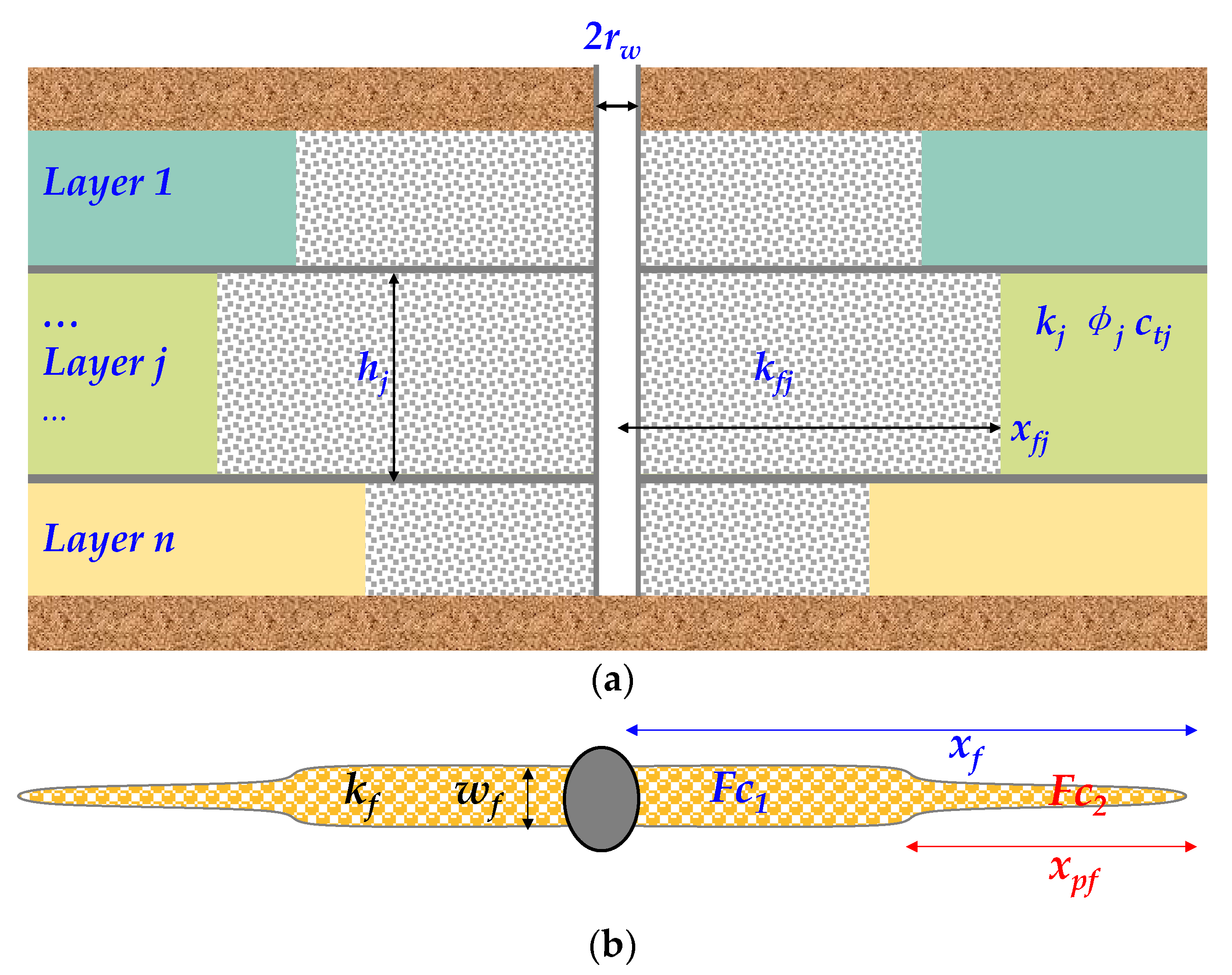
An MLVF commingled production well is located in a tight gas reservoir. Each layer has an individual constant thickness (hj), and vertical fracture length (xfj);
(2)
Any layer is penetrated by an MLVF commingled production well with height (ht) and radius (rw). The formation parameters belonging to any layer are different, such as the formation permeability (kj), formation porosity (φj), and reservoir total compressibility (ctj);
(3)
The formation porosity is filled with natural gas with constant viscosity (μ). The isothermal volume factor (B) is a constant value. The pressure (pj) and flow rate (qj) belonging to any layer are different due to the commingled production;
(4)
As shown in Figure 1b, the fracture width (wf) and fracture conductivity (Fc) is decreased from the wellbore to the toe of the fracture. In detail, the nearby fracture has higher conductivity (FC1) and more width than the further fracture. The further fracture has poor conductivity (FC2) and a smaller fracture length (xpf);
(5)
The gravity and temperature effects are ignored.

2.2. Mathematical Model

The reservoir pressure at the end of the fracture is equal to the fracture pressure at the end of the fracture. Therefore, the mathematical model includes the flow in the reservoir and the flow in the fracture region. In the reservoir region, the pressure in the reservoir can be obtained by the source solution of a vertical production well located at the infinite-acting reservoir. The dimensionless reservoir pressure of any layer j in the Laplace domain is:
p ¯ D j = 1 2 α j κ j α j α j q ¯ f D j K 0 [ ( x D x ) ω j κ j u ] d x
The parameters can be found in Table A1 in Appendix A.
In the fracture region, pressure is the key parameter in the fracture flow model. Similarly, the dimensionless pressure equation in the Laplace domain is rewritten as:
0 x D F c D j ( x D ) p ¯ f D j + π u α j κ j x D = 0 x D 0 x D π q ¯ f D j κ j α j 2 d x D d x D
where the parameters can be seen in Table A1. Appendix B gives the pressure semi-analysis solution at any discretized cell in the fracture region. The pressure at the fracture cell can be expressed as:
p ¯ f D n i + 1 / 2 = 1 2 α j κ j α j α j q ¯ f D j i K 0 [ ( x D i + 1 / 2 x ) ω j κ j u ] d x
For any fracture in layer j, there are n + 1 unknown parameter groups, i.e., [qfD1, …, qfDj, qfDn, pwDn]. Firstly, the unknown parameter groups can be calculated by the matrix Equation (A16) in Appendix C based on connection conditions in the cells of the fracture system. Then, the bottom-hole pressure can be calculated by the pressure and flow rate of all layers.
p ¯ w f D = 1 u ( j = 1 n 1 + u 2 C D j p ¯ w D j + u C D j S j κ j u p ¯ w D j + S j κ j ) 1
Based on the work of Van-Everdingen and Hurst [21], the dimensionless bottom-hole pressure can be obtained by the dimensionless rate solution in the Laplace domain:
p ¯ w D ( u ) = 1 u 2 q ¯ D ( u )
The Stehfest inversion is a classical method that transfers the value from Laplace domain to real-time domain (Stehfest, 1970) [22]. The pressure derivative can zoom the pressure features, the pressure derivative in the log–log coordinate system is:
p w D ( t D ) = t D d p w D ( t D ) d t D

3. Result and Discussion

In this part, all the solution equations of the mathematical model are achieved with Matlab 2021b. The Bessel function and numerical integral function are established by the default and self-written program code to obtain the value of bottom-hole pressure and its derivative. In the parts of type curves and the sensitivity analysis, all figures are drawn by Origin 2021 based on the value outputted by Matlab.

3.1. Solution Validation

When n = 1 (i.e., κ1 = 1, ω1 = 1, α1 = 1) and FcDj1 = FcDj2, the proposed model can be simplified as the conventional fracture well model with the finite conductivity presented by Cinco-Ley (1988) [10]. We compare the pressure and derivative results of the simplified model and Cinco-Ley’s model (1988) with different fracture conductivity. The fracture half-length is discretized into 10 equal-length cells. As shown in Figure 2, the proposed model matches well with Cinco-Ley’s model, indicating the proposed model’s correctness.

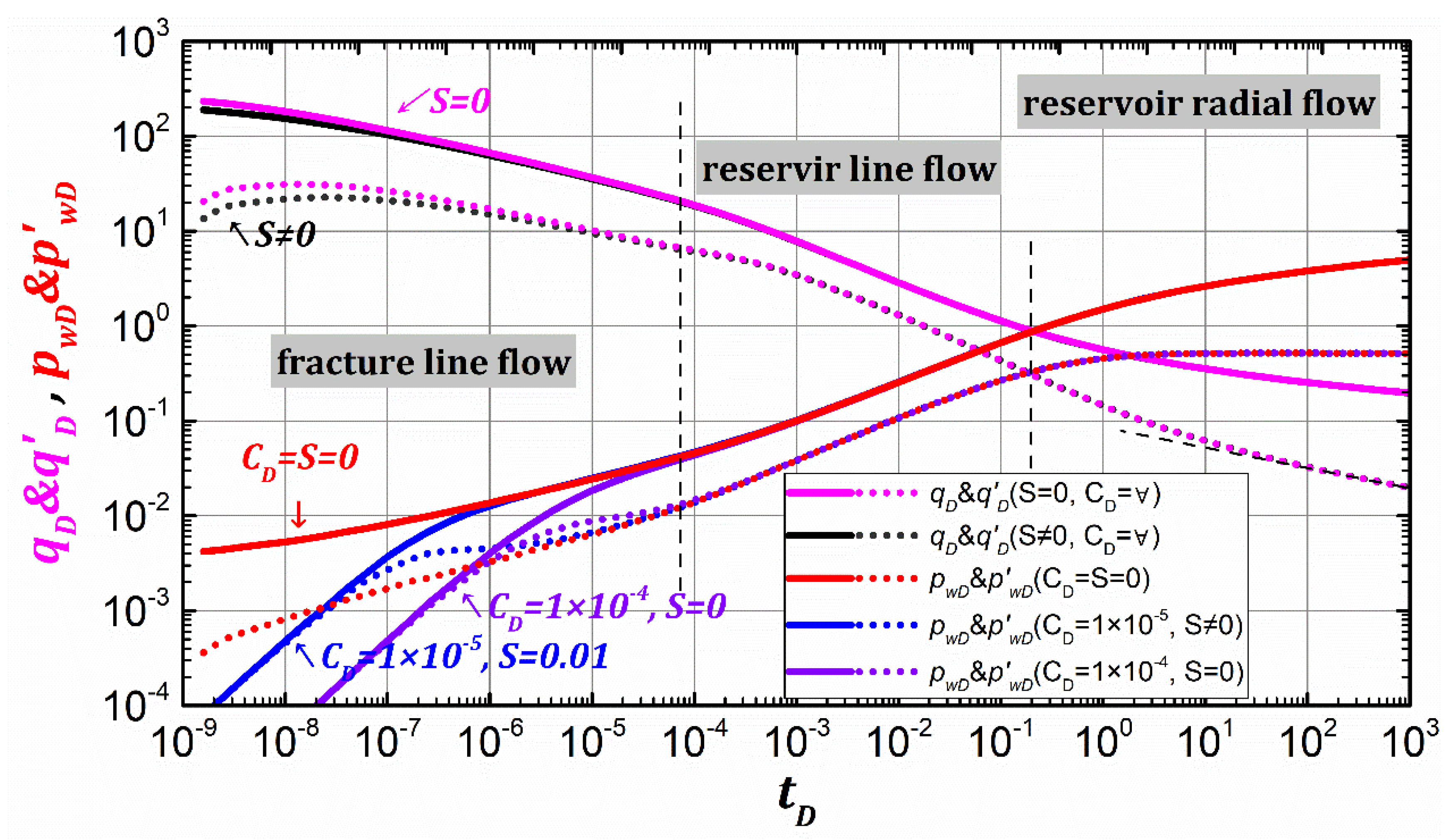
3.2. Combined Type Curve

To analyze the influence of wellbore, formation, and fracture on transient response behavior, we develop combined type curves by rate transient curve. The parameter’s value of the combined type curve can be found in Table 2. In detail, the wellbore parameter is the wellbore storage. The formation parameters include the skin, permeability ratio, and storability ratio. The fracture parameters include fracture length, conductivity, and extension.
The combined type curve includes the RTA type curves and the PTA curves. As shown in Figure 3, the pressure curve (pwD) and pressure derivative curve (p’wD) show that the flow of the MLVF well in the tight reservoir can be divided into five flow regimes. Correspondingly, the RTA combined type curves, rate curve (qD) and rate derivative curve (q’D), can also be divided into five stages. At any stage, the type curve features of PTA and RTA are shown in Table 3.

3.3. Sensitivity Analysis

On the one hand, the effect of the formation skin (S) on the combined type curves occurs in the very early stage. On the other hand, there is no effect of wellbore storage (CD) on the RTA type curves. Therefore, the CD and S are not considered and the two layers with the double conductivity fracture as a classical case were analyzed in the RTA sensitivity analysis part.

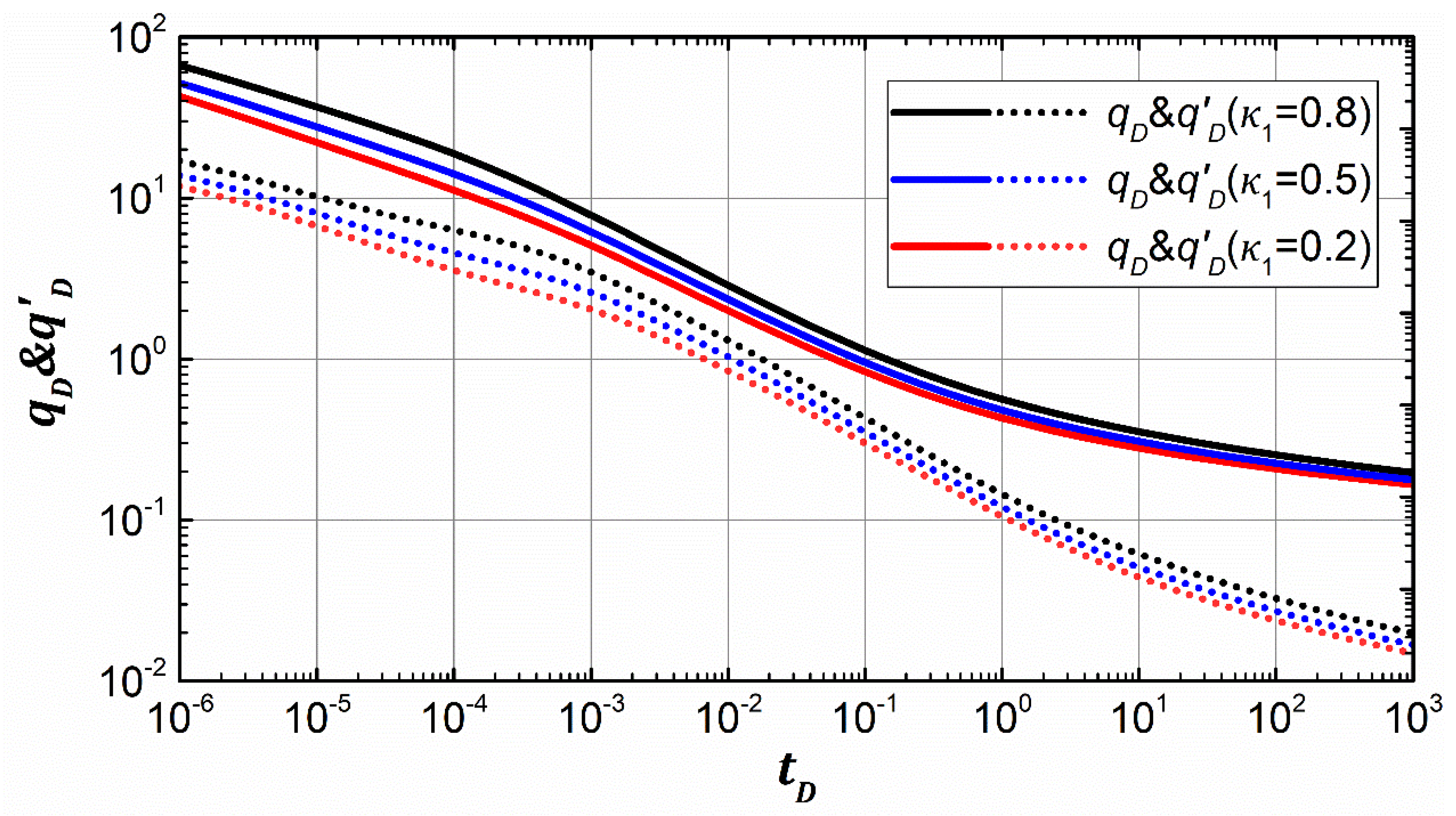
3.3.1. Formation Transmissibility

The value of formation transmissibility is determined by permeability and thickness. The transmissibility ratio is the ratio between one layer transmissibility and all layer transmissibility. As shown in Figure 4, the top layer transmissibility ratio (κ1) has an obvious effect on the rate transient behavior in the whole stage. The combined RTA curves move down with the decrease in the top layer transmissibility ratio. In a layered tight gas reservoir, improved well production can be achieved by enhancing the fracture permeability of the hydraulic fracturing process.

3.3.2. Formation Storability

Similarly, the value of formation storability is determined by compressibility and thickness. The storability ratio is the ratio between one layer’s storability and all layer storability. As shown in Figure 5, the top layer storability ratio (ω1) obviously affects the rate transient behavior in the middle stage. The combined RTA curves move up with the increase in the top layer storability ratio. For improving the well’s production, the effect is not obvious. In layered tight gas reservoirs, the effect of improving well production by increasing the fracture porosity during hydraulic fracturing is relatively insignificant compared to increasing fracturing permeability.

3.3.3. Fracture Length

The fracture length of the top layer is xf1, and the fracture length of the bottom layer is xf2. As the dimensionless definition is shown in Table A1, the fracture length ratio of the top layer (α1) is the ratio between xf1 and xf1 + xf2, i.e., Rp = xp1/(xf1 + xf2). With the top layer fracture length ratio increasing, the combined RTA curves move down. As shown in Figure 6, the top layer fracture length ratio (α1) affects the rate transient behavior in the whole stage, especially the early and middle stages. The combined RTA curves move up with the increase in the top layer fracture length ratio. This phenomenon shows that increasing the fracture length percentage of high permeability layers can obviously improve the well’s production of layered tight gas reservoirs.

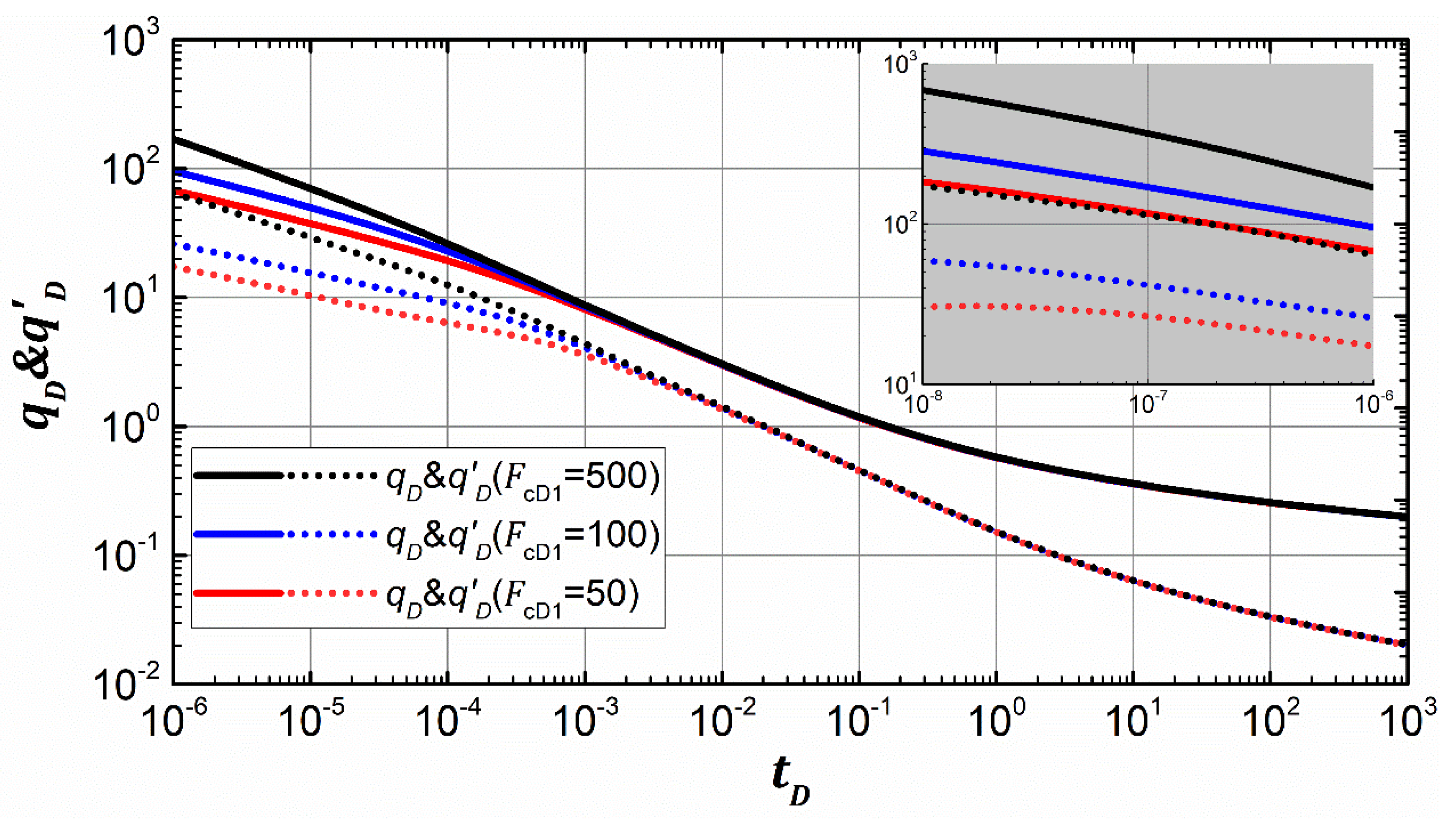
3.3.4. Fracture Conductivity

For any layer, the nearby dimensionless fracture conductivity (high conductivity) is FcD1. Similarly, the farther fracture conductivity (poor conductivity) is FCD2. In Figure 7, the poor conductivity (FcD2) is 50, and the combined RTA curves move up with the increase in high conductivity (FcD1). The high conductivity only affects the rate transient behavior in the early stage (see the small grey window). This result indicates the well’s production at the early stage is only sensitive to the nearby high fracture conductivity. Therefore, the enhanced well production cannot just be from increasing the nearby fracture to high conduction.

3.3.5. Fracture Extension

As shown in Figure 1b, the poor conductivity fracture length is xpf, and the fracture length is xf. Due to the definition of fracture extension as shown in Table A1, the fracture extension is the ratio of poor conductivity fracture length to the whole fracture length, i.e., Rp = xpf/xf. In Figure 8, the combined RTA curves move up with the decrease in the length of poor conductivity fracture (xpf). The high fracture extension only affects the rate transient behavior in the early stage (see the small grey window). Similar to the sensitivity of fracture conduction, the early well production is also sensitive to fracture extension. Combining the effects of fracture length and fracture conductivity, enhancing fracture whole permeability, and fracture length are the effective directions of enhancing the well’s production in the all-life production stage.

4. Conclusions

This paper presents an extended semi-analytical RTA model of a multi-layer fractured vertical well with a non-uniform fracture length and conductivity in the layered tight gas reservoir by the Laplace transform, Shehfest inverse, and Duhamel’s superposition principle, and further develops the combined type curves to capture the production behavior characteristics affected by a wellbore, formation, and fracture features. Several conclusions and suggestions are obtained from this work.
(1)
The rate transient behavior can be divided into three stages: the early stage, with −1/4 linear decreasing feature, the difference between rate and rate derivative is log4; the middle stage, with −1/2 linear decreasing feature, the difference between rate and rate derivative is log2; the later stage, the rate derivative curve is linearly decreasing.
(2)
The rate transient response is different from the pressure transient response, and wellbore storage has no effect on the rate transient behavior. On the other hand, the formation skin affects only the very early stages of rate transient behavior and the overall effect is not very large. Therefore, wellbore storage and formation skin do not need special consideration in the production decline analysis of multi-layer fractured vertical wells in tight gas reservoirs.
(3)
Reservoir transmissibility has an impact on the whole rate transient stage, and the storability mainly affects the middle stage of the rate transient response. As the formation transmissibility and storability increase, the combined RTA type curve moves upward, showing higher production and the influence of formation transmissibility is obviously larger than that of formation storability.
(4)
Fracture length has an impact on the whole rate transient stage, and fracture conductivity and fracture extension of high conductivity mainly affect the early stage of the transient rate. The longer the fracture length, the greater the fracture conductivity, the longer fracture extension of the high conductivity fracture, the higher the combined RTA curve, and the higher the production.

Author Contributions

Conceptualization, S.C.; methodology, C.Z.; validation, G.C.; investigation, K.Y.; writing—review and editing, Y.M.; funding acquisition, Y.W. All authors have read and agreed to the published version of the manuscript.

Funding

This research was funded by National Science Foundation for Young Scientists of China grant number 52104049.

Informed Consent Statement

Informed consent was obtained from all subjects involved in the study.

Conflicts of Interest

The authors declare no conflict of interest.

Nomenclature

BIsothermal volume factor, m3/m3
CWellbore storage factor, m3/Pa
cfFormation compressibility, Pa−1
cgGag compressibility, Pa−1
ctTotal compressibility, Pa−1
FCFracture conductivity
hThickness, m
kPermeability m2
K0Bessel function
nNumber of layers, positive integer
pPressure, Pa
piInitial formation pressure, Pa
pwBottom-hole pressure, Pa
qFlow rate, m3/s
QWell production, m3/d
RpFracture extension ratio
SSkin factor
tReal production time, s
uLaplace variable
wfFracture width, m
xX-axis distance, m
yY-axis distance, m
zGas compression factor
αFracture length ratio, fraction
μViscosity of the fluid, Pa·s
φPorosity, fraction
κTransmissibility ratio, fraction
ωStorability ratio, fraction
*DDimensionless parameters
*fFracture parameters
*jLayer j
*Derivate of parameters

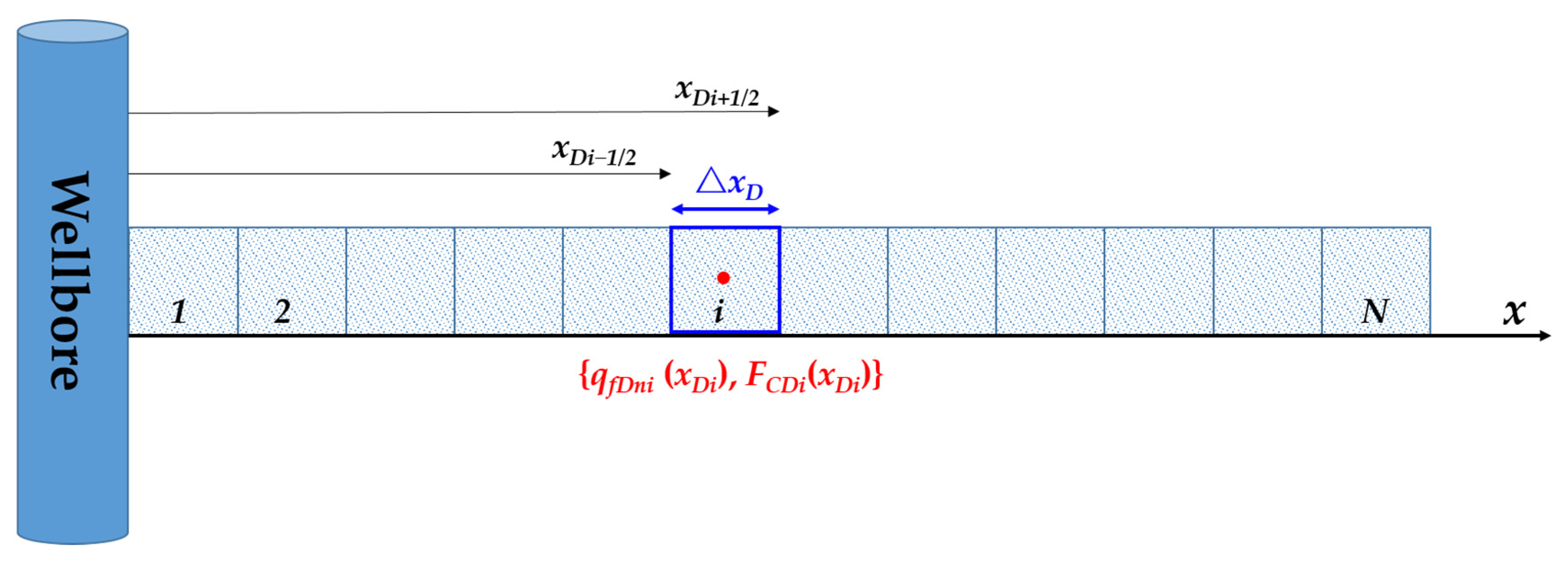
Appendix A. Reservoir Flow Model

According to Gringarten’s work (1973), we can easily give the point-source function of a well in infinite oil layer j with constant production rate qj.
p j = p j i 1 4 π ϕ j c f χ j h j 0 t q j ( τ ) t τ e x p [ ( x x ) 2 + ( y y ) 2 4 χ j ( t τ ) ] d τ
where χ = k ϕ μ c f is the diffusivity of layer j.
Let us regard the fracture as the line source. The pressure solution for a well intercepted by fracture is obtained by integrating Equation (A1) along the hydraulic fracture, given by:
p j = p j i 1 4 π ϕ j c f χ j h j 0 t x f j x f j q f j ( τ ) t τ e x p [ ( x x ) 2 + ( y y ) 2 4 χ j ( t τ ) ] d x d τ
where qfj is the flow rate per unit of fracture length going from the formation into the fracture of layer j.
Equation (A2) can be rewritten in the Laplace domain with dimensionless form, given by:
p ¯ D j = 1 2 α j κ j α j α j q ¯ f D j K 0 [ ( x D x ) ω j κ j u ] d x
where qfDj is defined as:
q f D j = 2 q f j x f j q j
The dimensionless definitions in the equation system, dimensionless variable, and definition are listed in Table A1.
Table A1. Dimensionless parameter and definition.
ParametersDefinitionParameters Definition
Dimensionless pressure p D j = k h ¯ 1.842 Q μ B [ 0 p 2 p d p μ z ] p j p i Dimensionless time t D = 3.6 × 10 3 k h ¯ ϕ h ¯ c t μ x ¯ f 2 0 t d t μ c g
Dimensionless rate q D j = q j Q Dimensionless fracture length α j = x f j x ¯ f
Dimensionless transmissibility factor κ j = ( k h ) j k h ¯ Dimensionless storability factor ω j = ( ϕ h ) j ϕ h ¯
Dimensionless wellbore storage C D = C 2 π ϕ h ¯ c t x ¯ f 2 Dimensionless fracture conductivity F c D j = k f j w f j k j x f j
Dimensionless distance x D = x x ¯ f ,   y D = y x ¯ f Dimensionless fracture extension R p j = x p f j x ¯ f
Note that the definitions k h ¯ = j = 1 n ( k h ) j , ϕ h ¯ = j = 1 n ( ϕ h ) j , x f ¯ = j = 1 n x f j are used in Table A1.

Appendix B. Fracture Flow Model

The flow occurs in the hydraulic-fracture region in the linear flow. The diffusivity equation is now formulated in terms of dimensionless variables in layer j. Note that we neglect the fluid compressibility inside the fracture due to the hydraulic-fracture volume being too small.
x D [ F c D j ( x D ) p f D j x D ] π q f D j κ j α j 2 = 0
The initial condition is:
p f D j ( t D = 0 ) = 0
The inner boundary and outer boundary conditions are:
p f D j x D | x D = 0 = π F c D j ( x D = 0 ) α j κ j
p f D j x D | x D = α j = 0
Integrating Equation (A8) from 0 to xD, the resulting equation is obtained with the boundary condition, given by:
F c D j ( x D ) p f D j x D + π α j κ j 0 x D π q f D j κ j α j 2 d x D = 0
Integrating Equation (A9) from 0 to xD again, the resulting equation is obtained with the boundary condition, given by:
0 x D F c D j ( x D ) p f D j + π α j κ j x D 0 x D 0 x D π q f D j κ j α j 2 d x D d x D = 0
Equation (A10) in the Laplace domain can be rewritten as:
0 x D F c D j ( x D ) p ¯ f D j + π u α j κ j x D = 0 x D 0 x D π q ¯ f D j κ j α j 2 d x D d x D
The dimensionless definitions in the equation system, Equation (A3) through Equation (A11), are listed in Table A1. Discretizing the fracture (half-length) into k equal-length cells with uniform flux, as shown in Figure A1, Equation (A11) can be written as:
i = 1 k F c D j i x D i 1 / 2 x D i + 1 / 2 p ¯ f D j + π u α j κ j x D j = π κ j α j 2 ( x D j i = 1 k q ¯ f D j i x D i 1 / 2 x D i + 1 / 2 x D i = 1 k q ¯ f D j i x D i 1 / 2 x D i + 1 / 2 x D x D )
Figure A1. Discretization scheme of fracture in layer n.
Energies 15 05705 g0a1
Equation (A12) can be further written as:
i = 1 k F c D j i ( p ¯ f D j i + 1 / 2 p ¯ f D j i 1 / 2 ) + π u α j κ j x D j = π κ j α j 2 ( Δ x D x D j i = 1 k q ¯ f D j i Δ x D i = 1 k q ¯ f D j i x D i )
where   Δ x D = α j / k , x D i = ( i 0.5 ) Δ x D , x D j = k Δ x D
The reservoir and fracture flow model are coupled by the pressure and flowrate continuity condition of every cell. We obtain the p ¯ f D j i + 1 / 2 by Equation (A3) for the j cell.
p ¯ f D j i + 1 / 2 = 1 2 α j κ j α j α j q ¯ f D j i K 0 [ ( x D i + 1 / 2 x ) ω j κ j u ] d x = 1 2 α j κ j i = 1 k x D i 1 / 2 x D i + 1 / 2 q ¯ f D j i { K 0 [ ( x D i + 1 / 2 + x ) ω j κ j u ] + K 0 [ ( x D i + 1 / 2 x ) ω j κ j u ] } d x

Appendix C. Solution of the Model

Combining Equations (A13) and (A14), we obtain an equation system with n Equations. The n + 1 unknowns for every cell are qfD1, …, qfDj, …, qfDn, and pwDn. There are n Equations and n + 1 unknowns. To solve the equation system, another equation is needed. Recalling that the flow entering the fracture is equal to the flow rate of the layer j, that is
i = 1 N q ¯ f D j = N u
The unknowns are found by solving the system of equations.
[ .. F c D j ( x D = 0 ) A i j .. .. F c D j ( x D = 0 ) 1 .. 1 0 ] [ .. q ¯ f D j i ( s ) .. p ¯ w D j ( s ) ] = B j
If the wellbore storage and skin effect are considered, we obtain the following equation based on the Duhamel theorem and the pressure superposition principle. Note that we consider each layer has a different wellbore storage coefficient and skin factor.
q ¯ D j = 1 + u 2 C D j p ¯ w D j + u C D j S j κ j u p ¯ w D j + S j κ j p ¯ w f D
where p ¯ w D j is given from Equation (A16). CDj and Sj are the wellbore storage coefficient and skin factor of layer j, respectively.
Finally, the bottom-hole pressure of the commingling system is obtained with the flowrate condition j = 1 n q ¯ D j = 1 / u in the Laplace domain, given by:
p ¯ w f D = 1 u ( j = 1 n 1 + u 2 C D j p ¯ w D j + u C D j S j κ j u p ¯ w D j + S j κ j ) 1
where total wellbore storage should be C D j = h j h j C D in this work.

References

  1. Denney, D. Challenges of Tight and Shale-Gas Production in China. J. Pet. Technol. 2013, 65, 153–156. [Google Scholar] [CrossRef]
  2. Sahin, A. Unconventional Natural Gas Potential in Saudi Arabia. In Proceedings of the SPE Middle East Oil and Gas Show and Conference, Manama, Bahrain, 10 March 2013. [Google Scholar] [CrossRef]
  3. McLennan, J.D.; Green, S.J.; Bai, M. Proppant Placement during Tight Gas Shale Stimulation: Literature Review and Speculation. In Proceedings of the 42nd U.S. Rock Mechanics Symposium (USRMS), San Francisco, CA, USA, 29 June–2 July 2008. [Google Scholar]
  4. Haghshenas, A.; Hamedpour, M. Well Performance Analysis in Shale/Tight Gas Reservoirs: Case Study Review. In Proceedings of the SPE Conference at Oman Petroleum & Energy Show, Muscat, Oman, 21–23 March 2022. [Google Scholar] [CrossRef]
  5. Muskat, M. The flow of homogeneous fluids through porous media. Soil Sci. 1938, 46, 169. Available online: https://blasingame.engr.tamu.edu/z_zCourse_Archive/P620_18C/P620_zReference/PDF_Txt_Msk_Flw_Fld_(1946).pdf (accessed on 12 July 2022). [CrossRef]
  6. Gringarten, A.C.; Ramey, H.J., Jr. The Use of Source and Green’s Functions in Solving Unsteady-Flow Problems in Reservoirs. Soc. Pet. Eng. J. 1973, 13, 285–296. [Google Scholar] [CrossRef]
  7. Gringarten, A.C.; Ramey, H.J., Jr.; Raghavan, R. Unsteady-State Pressure Distributions Created by a Well with a Single Infinite-Conductivity Vertical Fracture. Soc. Pet. Eng. J. 1974, 14, 347–360. [Google Scholar] [CrossRef] [Green Version]
  8. Cinco-Ley, H.; Samaniego, V.F.; Dominguez, N. Transient pressure analysis for a well with finite conductivity fracture. Soc. Pet. Eng. AIME J. 1978, 18, 253–269. [Google Scholar] [CrossRef] [Green Version]
  9. Cinco-Ley, H.; Fernando, S.V. Transient Pressure Analysis for Fractured Wells. J. Pet. Technol. 1981, 33, 1749–1766. [Google Scholar] [CrossRef]
  10. Cinco-Ley, H.; Meng, H.Z. Pressure Transient Analysis of Wells With Finite Conductivity Vertical Fractures in Double Porosity Reservoirs. In Proceedings of the SPE Annual Technical Conference and Exhibition, Houston, TX, USA, 2–5 October 1988. [Google Scholar] [CrossRef]
  11. Wei, C.; Cheng, S.; Tu, K.; An, X.; Qu, D.; Zeng, F.; Wu, D. A hybrid analytic solution for a well with a finite-conductivity vertical fracture. J. Pet. Sci. Eng. 2020, 188, 106900. [Google Scholar] [CrossRef]
  12. Luo, L.; Cheng, S.; Lee, J. Characterization of refracture orientation in poorly propped fractured wells by pressure transient analysis: Model, pitfall, and application. J. Nat. Gas Sci. Eng. 2020, 79, 103332. [Google Scholar] [CrossRef]
  13. Dou, X.; Hong, S.; Tao, Z.; Lu, J.; Xing, G. Transient Pressure and Rate Behavior of a Vertically Refractured Well in a Shale Gas Reservoir. Energies 2022, 15, 4345. [Google Scholar] [CrossRef]
  14. He, Y.; Cheng, S.; Rui, Z.; Qin, J.; Fu, L.; Shi, J.; Wang, Y.; Li, D.; Patil, S.; Yu, H.; et al. An Improved Rate-Transient Analysis Model of Multi-Fractured Horizontal Wells with Non-Uniform Hydraulic Fracture Properties. Energies 2018, 11, 393. [Google Scholar] [CrossRef] [Green Version]
  15. Zhao, K.; Du, P. A new production prediction model for multistage fractured horizontal well in tight oil reservoirs. Adv. Geo-Energy Res. 2020, 4, 152–161. [Google Scholar] [CrossRef]
  16. Xu, G.; Yin, H.; Yuan, H.; Xing, C. Decline curve analysis for multiple-fractured horizontal wells in tight oil reservoirs. Adv. Geo-Energy Res. 2020, 4, 296–304. [Google Scholar] [CrossRef]
  17. Zhang, J.; Cheng, S.; Zhu, C.; Luo, L. A numerical model to evaluate formation properties through pressure-transient analysis with alternate polymer flooding. Adv. Geo-Energy Res. 2019, 3, 94–103. [Google Scholar] [CrossRef]
  18. Wei, C.; Liu, Y.; Deng, Y.; Cheng, S.; Hassanzadeh, H. Analytical well-test model for hydraulicly fractured wells with multiwell interference in double porosity gas reservoirs. J. Nat. Gas Sci. Eng. 2022, 103, 104624. [Google Scholar] [CrossRef]
  19. Sun, B.; Shi, W.; Zhang, R.; Cheng, S.; Zhang, C.; Di, S.; Cui, N. Transient Behavior of Vertical Commingled Well in Vertical Non-Uniform Boundary Radii Reservoir. Energies 2020, 13, 2305. [Google Scholar] [CrossRef]
  20. Shi, W.; Yao, Y.; Cheng, S.; Shi, Z. Pressure transient analysis of acid fracturing stimulated well in multilayered fractured carbonate reservoirs: A field case in Western Sichuan Basin, China. J. Pet. Sci. Eng. 2019, 184, 106462. [Google Scholar] [CrossRef]
  21. Van Everdingen, A.F.; Hurst, W. The Application of the Laplace Transformation to Flow Problems in Reservoirs. J. Pet. Technol. 1949, 1, 305–324. [Google Scholar] [CrossRef]
  22. Stehfest, H. Numerical inversion of Laplace transforms. Commun. ACM 1970, 13, 624. [Google Scholar] [CrossRef]
Figure 1. Physical model of MLVF well in a tight gas reservoir. (a) Formation model; (b) Double conductivity vertical fracture model.
Energies 15 05705 g001
Figure 2. Comparison of the proposed model and Cinco-Ley’s model under different fracture conductivity.
Energies 15 05705 g002
Figure 3. Combined type curves of MLVF well in a tight gas reservoir.
Energies 15 05705 g003
Figure 4. RTA type curves of formation transmissibility ratio.
Energies 15 05705 g004
Figure 5. RTA type curves of formation storability ratio.
Energies 15 05705 g005
Figure 6. RTA type curves of fracture length ratio.
Energies 15 05705 g006
Figure 7. RTA type curves of fracture conductivity ratio.
Energies 15 05705 g007
Figure 8. RTA type curves of fracture extension.
Energies 15 05705 g008
Table 1. The average value of reservoir parameters for fractured wells in Sulige tight gas field.
Hydraulic Fracturing TypeNet Pay
(m)
Porosity
(%)
Permeability
(10−3 μm2)
Gas Saturation
(%)
Absolute Open Flow
(104 m3/d)
4 layers11.210.90.6366.89.01
2 layers10.111.40.7771.96.11
Commingled fracturing9.910.90.6573.35.27
Table 2. The parameters of the combined type curve and sensitivity analysis curve.
Dimensionless ParametersValue
Type CurveSensitivity Analysis
WellboreDimensionless wellbore storage (CD)1 × 10⁻⁵/
FormationSkin factor (S)0.01/
Permeability ratio (κ)0.50.2, 0.5, 0.8
Storability ratio (ω)0.50.3, 0.5, 0.7
FractureDimensionless fracture length (α)0.50.1, 0.3, 0.5, 0.7, 0.9
Dimensionless fracture conductivity (FCD)5050, 100, 500
Dimensionless fracture extension (RD)0.50.1, 0.3, 0.5, 0.7, 0.9
Table 3. The parameter values of the analysis part of this work.
Transient Behavior StagesCombined Type Curves Feature
PTARTA
Wellbore storage M = 1, dp = 0/
Skin transient //
Fracture line flow m = 1/4, dp = log4m = −1/4, dq = log4
Reservoir line flow m = 1/2, dp = log2m = −1/2, dq = log2
Reservoir radial flow p’wD = 0.5m = tanθ
Note: m = slope, dp = log(pwD) − log(p’wD), dq = log(qD) − log(q’D).
Publisher’s Note: MDPI stays neutral with regard to jurisdictional claims in published maps and institutional affiliations.

