The Environmental Profile of Ethanol Derived from Sugarcane in Ecuador: A Life Cycle Assessment Including the Effect of Cogeneration of Electricity in a Sugar Industrial Complex

Abstract

The present study compiles a life cycle inventory for Ecuadorian sugarcane-derived ethanol production to quantify its environmental performance and identify the life cycle stages that cause major impacts. The scope of this study encompasses a cradle-to-gate analysis that includes the agriculture, the milling, the distillation, and the co-generation of electricity. This assessment is modeled using the OpenLCA v1.10.3 software. Two functional units (FU) were established in this study: “1 ton of sugarcane at-the-farm-gate” for the agricultural stage and “1 L of ethanol at-the-plant-gate”. A hybrid attributional and consequential life cycle analysis (LCA) approach has been followed. Economic allocation (EA) and system expansion (SE) were used to take co-products into account in the milling and co-generation of electricity stages, respectively. The co-generation stage is analyzed in three different scenarios: (i) average mix displacement scenario where the surplus electricity produced in the co-generation stage is displaced; (ii) marginal technology displacement scenario where the marginal surplus electricity is displaced from the mix and (iii) no displacement scenario. The global warming potential (GWP) impact at the farm gate level was reported as 53.6 kg of carbon dioxide equivalent (kg ${\mathrm{CO}}_{2\mathrm{eq}.}$) per ton of sugarcane produced. The two main contributors of the agricultural stage correspond to N₂O lixiviation and volatilization with 34% followed by the diesel used in agricultural machinery with 24%. The GWP for 1 L of ethanol produced was reported as 0.60 kg ${\mathrm{CO}}_{2\mathrm{eq}.}$ based on the average mix displacement scenario. No displacement scenario has a GWP impact of 0.84 kg ${\mathrm{CO}}_2$/liter of ethanol The distillation stage has the highest contribution to GWP impact with approximately 61% followed by the agricultural stage with 47%. The co-generation stage reports a contribution of −8.4% due to the surplus electricity displacement. The scenarios where the system expansion method is applied have a lower GWP impact compared to the scenario where no surplus electricity is displaced. Regarding terrestrial acidification potential impact, 0.01528 kg of ${\mathrm{SO}}_{2\mathrm{eq}.}$ was reported at the ethanol production level especially due to the nitrogen and phosphorous content in the vinasse produced from the distillation process. The marine eutrophication impact for 1 L of ethanol produced was 0.00381 kg of ${\mathrm{N}}_{\mathrm{eq}.}$ due to the content of nitrogen contained in the vinasse and the use of nitrogenous fertilizers in the agricultural stage. Finally, to create more eco-friendly Ecuadorian sugarcane and ethanol industries, sustainable and less polluting processes should be sought to reduce the environmental burdens. Companies should apply industrial symbiosis and circular economy strategies to produce lesser environmental loads within the ethanol production chain. The sugarcane industrial sector should also promote the surplus electricity production in order to gain credits.

1. Introduction

1.1. Worldwide Biofuels Context

Nowadays, there is a rising awareness about the future mitigation of fossil resources [1]. There is a general scientific consensus that the observed trends in global warming have been caused by the indiscriminate use of fossil fuels in human activities. The latter is threatening the global environment. For instance, more interest is beginning to be shown in the emergence of alternative sustainable energy sources [2].

Biofuels have been recognized as an alternative to reduce the consumption of fossil fuels and thus help to decrease greenhouse gas (GHG) emissions [3]. In 2018, global biofuels production reached 153 billion liters, increasing 7% compared to 2017 [4]. Biofuels account for approximately 3% of the global transportation sector [5]. The insertion of biofuels in the worldwide transportation has been slowly dosed due to the potential risk of globally reducing food production by allocating more arable lands for energy crops production [6,7,8,9].

Although many countries have promoted and implemented biofuels to address energy security and a more environmentally friendly economy [10,11], few scientists have suggested that biofuels development has been harmful to the environment, regardless of the country where it is produced [8]. The latter is justified because some crops can generate even more greenhouse gases than fossil fuels, depending on their production’s feedstock and fuel processes [12]. Additionally, some emissions and environmental impacts are produced at other stages, as in the production of inputs used for crops and biofuels: pesticides, herbicides, and fertilizers for crop production; chemicals production for biofuel processing, and emissions produced from transport and distribution to the field and industrial plants for crops and biofuels processing [13]. On the other hand, it is also essential to consider the emissions that can be generated from land-use change, triggered by increased biofuel production. The main effects of land-use changes are that the carbon dioxide accumulated in its vegetation escapes into the atmosphere, altering the impact of global warming [14]. For instance, a more detailed analysis of the environmental impacts of biofuels production is essential to have more solid evidence for policymakers to support biofuels development.

One of the main challenges in the agricultural sector in terms of sustainability is to mitigate the dependence on non-renewable resources to reduce emissions [15,16]. For instance, the industrial symbiosis (IS) term has gained strength lately in this sector. Several countries around the world are strongly applying industrial symbiosis due to its economic and environmental benefits. For example, nitrogen fertilizers are manufactured using non-renewable resources, and are an important outlet for fossil fuels [17]. Thus, industrial symbiosis enables these non-renewable inputs to be replaced through fertilizers sourced from organic waste such as vinasse and filter cake [18,19]. Valorization of lignin-rich stream from industrial-scale lignocellulosic ethanol [20], the aqueous phase reforming of glucose and xylose for hydrogen production [21] and the hydrogen production from sugar beet molasses through dark fermentation, photo-fermentation, and gas upgrading [22] are other examples of industrial symbiosis in the sugar industry. Furthermore, agricultural sector companies have also been encouraged to cogenerate electricity by burning sugarcane bagasse in sugar industrial complexes [23,24]. This approach allows companies to mitigate environmental impacts produced during sugar production chain, and it also allows to increase their product portfolios.

Biofuels production from agriculture or industrial wastes has been encouraged as an alternative renewable energy source. Bioethanol is the most common and worldwide developed biofuel, mainly in the American continent, which has a significant potential to replace gasoline as a vehicle fuel (E5 to E100) in light-duty vehicles or ${\mathrm{ED}}_{95}$ in heavy-duty vehicles (${\mathrm{ED}}_{95}$ is a fuel grade containing up to 95% ethanol [25]. With light-duty vehicle electrification, it is still possible to use the ethanol in ${\mathrm{ED}}_{95}$ bus or goods transport and also as SAF (Sustainable Aviation Fuel). The aviation sector is also seeking biofuels penetration up to 50% in 2030 and 100% in 2050. The International Air Transportation Association (IATA), which represents major global airlines, has committed to net-zero carbon emissions from global air transportation by 2050. The International Civil Aviation Organization (ICAO) under the CORSIA [26] scheme embraces ethanol as a possible feedstock sugarcane derived-ethanol, that is subsequently converted to drop-in fuel via dehydration, oligomerization, and hydrotreating. The agreed default core LCA value for sugarcane ethanol is 24.1 ${\mathrm{gCO}}_{2\mathrm{eq}.}/\mathrm{MJ}$, while reference fossil jet fuel is 89 ${\mathrm{gCO}}_{2\mathrm{eq}.}/\mathrm{MJ}$, accounting for transportation logistics and jet fuel burning in the airplane. From REDII Annex VI [27], the GHG savings for biomethane relative to the fossil fuel comparator for transport is 94 g ${\mathrm{CO}}_{2\mathrm{eq}.}$/MJ.

Traditionally, sugarcane has mainly been processed to obtain sugar for human consumption [24]. However, it has also long been recognized as producing other products such as electricity, fuels, organic chemicals, and paper [28]. The recognition of sugarcane as a renewable energy source, biofuel, biomaterials, and food crops [29,30] has produced a greater scientific interest in sugarcane products’ life cycle environmental impacts.

Sugarcane biorefinery [31] for sugar, ethanol, heat, and electricity is the best configuration in terms of circular economy and energy transition.

1.2. Life Cycle Assessment of Biofuels

The Life Cycle Assessment (LCA) is an environmental management tool to assess the burdens associated with a product or service during its entire life cycle [32]. The LCA has been broadly used to quantify the environmental burdens of different transportation biofuels to estimate the net effects of biofuel on several impact categories such as climate change, freshwater eutrophication, marine ecotoxicity, fossil resource scarcity, and water consumption [33,34,35,36,37]. Sydney et al. [34] analyzed the reduction in worldwide greenhouse gases emissions through a cradle-to-grave life cycle assessments for corn, sugarcane, and beet ethanol, while Yan et al. [36] developed a comparative life cycle assessment analysis on ethanol produced from agave, corn, and sugarcane. Moreover, these assessments can be used to compare biofuels against conventional petroleum-derived fuels such as gasoline, diesel, and aviation fuels [38,39]. Reviews of the environmental impacts of different biofuels are subject to significant biases associated with the methodology applied, making it difficult to compare the results on a rational basis [40]. These biases derive from criteria modeling choices regarding system definition and boundaries, functional unit definition, reference systems, and co-product allocation methods [41,42,43,44,45,46,47]. Even so, some LCA studies differ in selecting life cycle impact assessment methods [48,49,50,51,52,53]. For instance, Elsayed et al. [46] developed a Well-to-Tank (WTT) LCA of different fuel options (gasoline, diesel, crude naphtha, compressed natural gas, methanol, Fischer–Tropsch naphtha, Fischer–Tropsch diesel, gaseous hydrogen, liquid hydrogen and ethanol) through a system expansion and defined 1 Megajoule as the functional unit. On the other hand, Wallace et al. [42], and Macedo et al. [47] performed a Well-to-Wheels (WTW) LCA of ethanol fuel using a system expansion, but they differ in selecting the functional unit (1 km and 1 ton of feedstock, respectively).

Raw Material and Conversion Technology Differences on Biofuels Reviews

Biofuels are classified into three groups: the first generation (1G), which are derived from grown edible plants; second-generation (2G), which are produced from non-edible crops, and third-generation (3G), which are produced from algae and other microorganisms [54], depending on the raw material and the conversion technology [55]. In addition, 4G biofuel can also be considered if involving genetic engineering. Despite being an excellent substitute for gasoline, sugarcane and maize, used as raw materials to produce ethanol, constitute between 40% and 70% of the ethanol production costs [56,57]. Moreover, first-generation (1G) ethanol production represents an ethical problem due to land food competition and being water-intensive [58,59,60]. Nevertheless, many ethanol LCA studies focus on 1G bioethanol [48,50,61,62,63,64]. On the other hand, cellulosic technology has been developed to convert 2G ethanol from lignocelluloses biomass rather than sugar or starch [65]. Thus, the ethical conflict with food competition and energy demand is somehow reduced. However, one of the main reasons this conversion technology does not contribute worldwide in a considerable manner is the high production cost [66]. Some LCA studies of 2G bioethanol as a vehicle fuel have been conducted using bagasse, molasses, corn stover, and switchgrass as raw materials [48,59,67,68,69,70,71,72].

1.3. Biofuels in Ecuador

Ecuador possesses an abundant biomass potential from crops, including their residues and livestock activities residues from poultry, swine, and cattle [73]. Several conversion technologies can convert this biomass into biofuels or other energy carriers. Regarding biodiesel fuel, the Ecuadorian government began producing this biofuel from African palm in 2005. Concerning bioethanol fuel, its production started in 2010 with Ecopais gasoline.

1.3.1. Bioethanol in Ecuador

In Ecuador, ethanol comes mainly from the sugarcane industry [74]. The Ecopaís Pilot Program (E5 = 5% v/v ethanol content in gasoline by volume type rated above 85 octanes) started in Guayaquil and Durán cities. Initially, the government aimed to increase the ethanol blend with gasoline from 5% to 10% by 2016, focusing the sugarcane expansion on coastal cities [75]. However, 400 million liters of ethanol are needed per year to reach this target, and the area of sugarcane crops should be extended by 500 km². It must be highlighted that around 79% of the industrial sugarcane crops are currently widespread in the Guayas Province [73]. Currently, the EcoPais fuel is sold in approximately 58% of the national territory [76]. This accomplishment was possible due to the expansion of the agricultural frontier and the investment of sugar mills to construct distillation plants for energy purposes. The three prominent sugar companies that produce most Ecuadorian ethanol are Valdez, San Carlos, and Coazucar.

1.3.2. Life Cycle Assessment of Energy Systems in Ecuador

Several LCA studies have been developed and applied to Ecuador’s energy, transportation, and materials [74,77,78,79,80,81,82,83,84,85,86]. Ramirez et al. [78], analyzed the environmental sustainability of current (from 2012 to 2018) and forecasted electricity generation and supply scenarios using a life cycle approach. Briones et al. [79], presented a complete life cycle environmental performance of two hydropower schemes in Ecuador regarding electricity LCA studies. Moreover, Briones et al. [77] determined the net environmental performance of hydropower through a methodological approach that combines and balances two well-known environmental-ecological assessments: life cycle (LCA) and ecosystem services assessment (ESA). Ramirez et al. [84], examined the potential environmental impact of fossil-based electricity generation technologies used in Ecuador, through ISO standards and CML 2000 methodology. Muñoz Mayorga et al. [85] have developed a comparative life cycle assessment of electricity produced from jatropha oil (JO) in Floreana Islands under three different systems. The analyzed systems include a blended system (BS) with 20% JO and 80% diesel, a reference system consisting of 100% diesel, and a jatropha system (JS) made up of JO. Parra et al. [83], explored the electricity produced in Galapagos from refined palm oil (RPO) produced in continental Ecuador and local waste cooking oil (WCO) using a comparative life cycle assessment methodological framework. Compared to refined palm oil, the results show better environmental performance in all the impact categories for the electricity produced from waste cooking oil. Ramirez et al. [81] quantified the change in the carbon footprint of the household cooking system from the current based on liquefied petroleum gas to the proposed based on electricity, using the LCA methodology.

Few LCA studies have focused on the environmental impacts of Ecuador’s biofuels production, providing little knowledge and guidance for decision-makers in the country’s energy sector [74,86,87]. Banana industry wastes have been explored as another potential source of ethanol in Ecuador [86,87]. These studies claim that Ecuador can produce an additional 118–266 L of ethanol per hectare yearly from this feedstock. The latter represents an extra 40 million liters of ethanol per year. Noteworthy is that approximately 150,000 hectares are destined for banana production in Ecuador. On the other hand, Chiriboga et al. [74] determined the Energy Return on Investment (EROI) for bioethanol and biodiesel, including three raw materials for ethanol (sugarcane, corn, and forest residues) and four for biodiesel (African palm, pinion, bovine fat, and swine fat). The authors also developed an LCA for the mentioned biofuels. Despite these latter three LCA studies, the environmental profile of sugarcane-derived ethanol has not been studied with a life cycle perspective. Regarding fossil gasoline and according to [88,89] the GHG emissions for refinery activities were 5.46 ${\mathrm{g}\mathrm{CO}}_{2\mathrm{eq}.}/\mathrm{MJ}$.

There is currently no way to assess the environmental impact of using ethanol as an energy vector in the Ecuadorian road transportation from a life cycle perspective. There are also lack of studies on the environmental profile of sugarcane, which is the main feedstock for producing ethanol in Ecuador.

1.4. Aim of the Study

The present study compiles a real-life cycle inventory for Ecuadorian sugarcane and sugarcane-derived ethanol production to quantify its environmental performance. This work considers the life cycle stages for 1G ethanol production: (i) agricultural, (ii) milling (iii) distillation, and (iv) electricity co-generation stages, to identify the critical processes that cause the major impacts. This study also aims to analyze the effect of electricity co-generation produced in the sugar industry complex on the environmental profile of ethanol.

2. Materials and Methods

The International Organisation for Standardisation (ISO) provides the LCA standards through the ISO 14040 and 14044 [90,91]. The LCA methodology consists of four stages: goal and scope definition, inventory analysis, impact assessment, and interpretation.

2.1. Goal and Scope Definition

This study evaluates sugarcane-derived ethanol production’s environmental performance based on Ecuadorian conditions. The life cycle stages considered for this analysis are related to the agricultural, milling, distillation and co-generation stages (Figure 1). The production pathway of this study produces ethanol from sugarcane juice mixed with molasses obtained within the milling stage. This pathway also produces sugar and vinasse through the milling and distillation stages, respectively. The inventory was gathered from a real Ecuadorian sugar mill company and an alcohol distillation plant. The national electricity mix is composed of 92% of hydropower generation and 7% of thermal power generation with a ${\mathrm{CO}}_{2\mathrm{eq}.}$ intensity of 0.0115 kg ${\mathrm{CO}}_{2\mathrm{eq}.}/$kWh and 3.3 kg ${\mathrm{CO}}_{2\mathrm{eq}.}/$kWh, respectively [78]. The remaining 1% corresponds to unconventional resources generation such as wind and solar technologies.

It is worth mentioning that worldwide there are different technologies and processes for converting sugarcane into ethanol and electricity, depending mainly on the agricultural practices of each country [59,92,93]. The two functional units (FU) used in this study are defined as “1 ton of sugarcane at-the-farm-gate” for the agricultural stage and “1 L of ethanol at-the-plant-gate”. The functional unit is a quantified description of the performance requirements that the product system fulfills. Moreover, the functional unit also serves as the reference basis for all environmental impact calculations and comparison with other systems with the same function.

The scope of this study embraces all the activities for ethanol production, enabling a cradle-to-gate analysis. The whole system includes the extraction of raw materials within the agricultural stage and ends with the final product (ethanol) at the gate of the distillery plant. The resource consumption, materials (except building materials and capital equipment), and energy inputs used during sugarcane cultivation, transportation, milling, and final conversion are considered for this analysis. We have not considered the impact associated with the production of capital equipment nor the storage and transportation tasks after ethanol production.

Economic allocation (EA) and system expansion (SE) were used to take co-products into account in the milling and co-generation stages, respectively. The co-generation stage considers three different scenarios of system expansion presented in

Table 1. System expansion scenarios for the co-generation stage.

Scenario	Description	Type of Generation Displaced
Average mix displacement	The surplus electricity generated in the co-generation stage is sold to the national electricity grid.	Average electricity mix
Marginal technology displacement	The surplus electricity generated in the co-generation stage is sold to the national electricity grid.	Internal combustion engine operating on fuel oil
No displacement	The effect of the surplus electricity generated is not considered.	Not applicable

. The system expansion method, also called the displacement or substitution method, was historically proposed to avoid allocation [94]. This method is a consequential approach that tends to represent the actual effects of generating multiple products from a pathway. The environmental burdens of producing the displaced products are credits that are then subtracted from the total environmental burdens of the production cycle.

The average mix displacement scenario is assumed as the more realistic one compared with the marginal technology displacement scenario and the scenario without surplus electricity displacement. The latter is justified with the Organic Law of the Public Service of Electricity, which establishes that the Ecuadorian government, through the Electricity and Renewable Energy Ministry, may delegate—exceptionally—to private capital companies, the contribution to the electricity sector activities, when it comes to projects that use non-conventional renewable energies such as biomass [95,96].

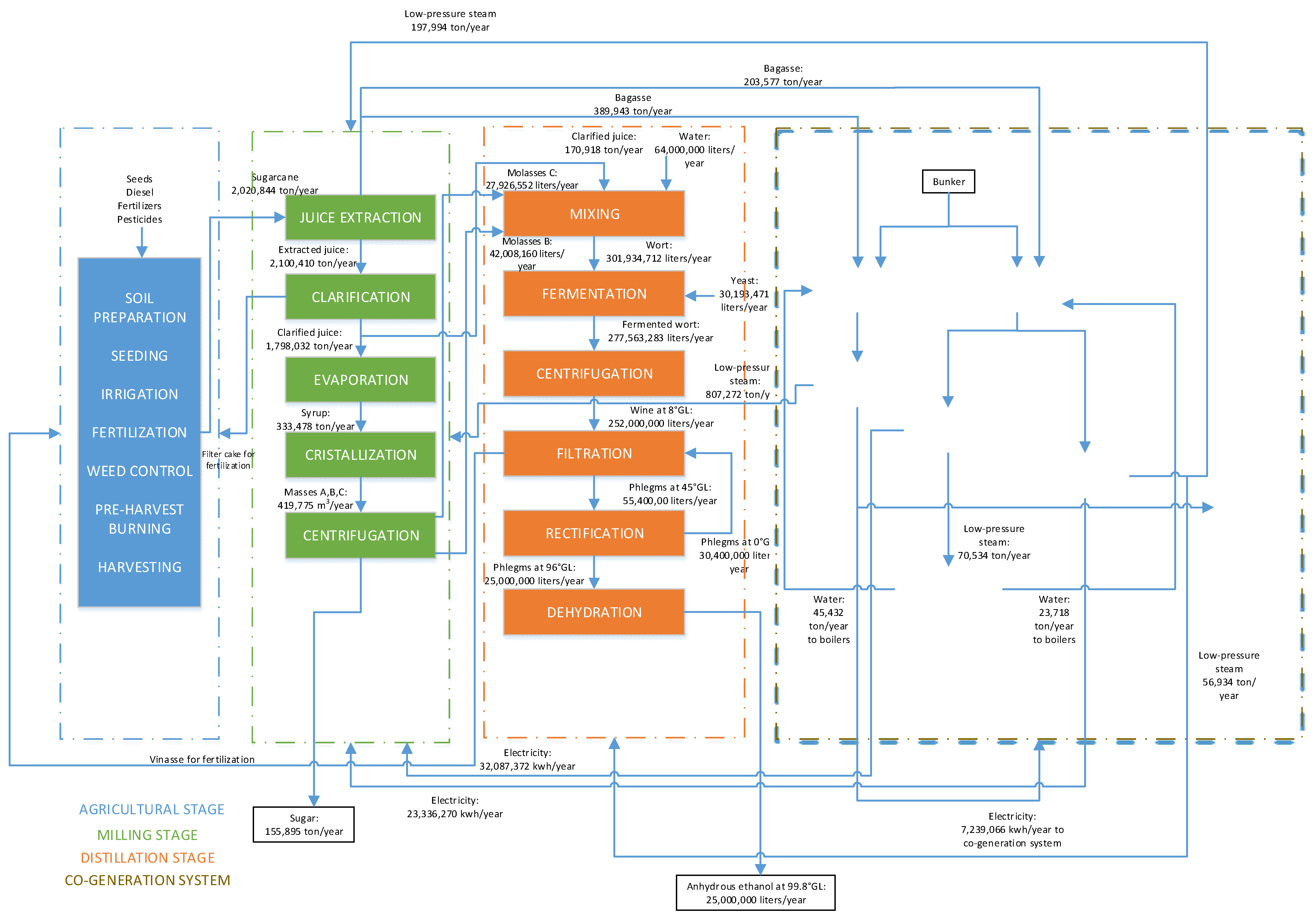
2.2. Life Cycle Inventory

The life cycle inventory (LCI) stage is the methodology step that includes the compilation of an inventory of inputs and outputs of a product system. The LCI of the ethanol production system was obtained from different sources. The inventory was developed based on primary data collected from a sugar mill company concerning the agricultural and milling stage. For the distillation stage, the data was collected from an alcohol distillation company and supplemented with secondary data from peer-reviewed literature [97,98]. It is noteworthy that these two companies are two of the largest in the Ecuadorian sugar and alcohol industries. The system description and inventory data are valid for sugarcane-based bioethanol in the coastal region of Ecuador and for the time framework 2017–2018.

The production of different co-products is a particular feature in the ethanol production chain. For this reason, methods such as allocation and system expansion are used to apportion the impacts generated by its production. The selection of the used method directly affects the results [48,64]. In this work, the economic allocation has been considered primarily in the milling stage, at the centrifugation process, where some co-products (sugar and molasses) are generated in the process.

2.2.1. Agricultural Stage

The agricultural stage includes soil preparation, seeding, irrigation, fertilization, weed control, and harvest. Soil preparation includes leveling, clearing, and plowing with a ripper and a subsoiler. The soil needs to be prepared at least once every five years. Like soil preparation, seeding is usually done once every five years, and the plowing phase can be performed either by hand or by machinery. For the irrigation phase, a period of around 7 to 8 months is generally necessary using pivots, water cannons, or a gravity system. The fertilization, weed control, and harvesting processes are usually performed once per year, either by hand or machinery. Generally, based on an Ecuadorian context, 100% of the sugarcane field is burned before each harvest process to perform the operations efficiently.

The agricultural stage inputs mainly include land, diesel, seeds, water, electricity, fertilizers, and agrochemicals (pesticides, herbicides, etc.). Among the outputs, the emissions generated in each process are primarily due to fossil fuel burning and fertilizers.

In cropland areas, only non-${\mathrm{CO}}_2$ emissions are considered since ${\mathrm{CO}}_2$ emissions are balanced with the emissions that are captured by the annual plant re-growth [99]. Emissions of gases such as carbon monoxide (CO), methane (${\mathrm{CH}}_4$), nitrogen species (${\mathrm{N}}_2\mathrm{O}$, ${\mathrm{NO}}_{\mathrm{x}}$), and non-methane volatile organic compounds (NMVOC), referred to as diesel combustion on agricultural machinery used for soil preparation, seeding, fertilization, weed control, and harvesting and agricultural residues burning, were considered [100]. For calculating non-${\mathrm{CO}}_2$ emissions due to the agricultural residues burning, the emission factors suggested by the Intergovernmental Panel on Climate Change (IPCC) were applied [101]. Other emissions to soil and water were calculated using the Life Cycle Inventories of Swiss and European Agricultural Production Systems Report [97].

Direct and indirect emissions generated through the application of synthetic nitrogen fertilizers were calculated in this study. The amount of fertilizers annually used by the company (2018) was reported as 280 kg/ha for urea, diammonium phosphate as 20 kg/ha, and potassium muriate as 65 kg/ha. The total sugarcane cropped area of the mill in 2018 was 28,500 hectares (ha), resulting in 2,020,844 tons of sugarcane and a crop yield of 70.91 t/ha.

The inventory for the agricultural stage is shown in detail in Table S1 in the Supplementary Material.

2.2.2. Milling Stage

The milling stage includes sugarcane milling, juice clarification, evaporation, crystallization, centrifugation, and drying processes to obtain sugar and molasses as the final products. The first sub-stage aims to obtain sugarcane juice. In the sugarcane juice extraction, the bagasse can be obtained, separated, and sent to the boilers to generate electricity and steam in the co-generation power plant. The extracted juice can also be used to produce sugar and molasses through several processes (clarification, concentration, and crystallization). This extracted juice can also be directly diverted to a fermentation process to obtain ethanol.

The milling stage inputs mainly include water and some chemicals such as phosphoric acid, sulfur, lime, and calcium hydroxide at the rate of 9.40, 263.8, 1140.8, and 230.3 kg/1000 tons of sugarcane, respectively.

The final products are sugar and molasses (B and C), which can be used in the ethanol production phase (distillation stage). Based on the milling stage, which produces more than one product, an economic allocation was used to fraction the flows of this process to the product system under study. For sugar product, a value of USD 33 for a sack of 50 kg was used for the allocation. In terms of molasses, values of USD 0.60 and USD 0.18 were used for molasses B and molasses C, respectively.

The inventory for the milling stage is shown in detail in Table S2 in the Supplementary Material.

2.2.3. Distillation Stage

Ethanol can be obtained directly from sugarcane juice or by mixing sugarcane juice with molasses (B and C) delivered during the milling process. The sugar and the remaining molasses from the milling stage are co-products that were not used in the production of ethanol. For this case, the wort obtained from the mixing process comes mainly from the sugarcane juice (71%), followed by the molasses B (18%) and by the molasses C (11%). This latter proportion allows to classify this ethanol as a first generation (1G). The molasses is mixed with sugarcane juice and fermented by yeast cultures. The amount of yeast used for the fermentation process was 1020 kg/year. Urea is used as a nitrogen source for the yeast production [102]. Finally, after the fermentation process, the fermenter wash is pumped to the distillation unit, where the produced wine is distilled and rectified to obtain anhydrous ethanol at 99.8° of alcoholic grade. The inventory data for this stage was obtained directly from one distillation plant. The electricity consumption of the distillation plant was 12,540,222 kW per the analyzed year. This distillation plant produced 25 million liters of ethanol in 2018. In 2021, the national ethanol production was planned to be 110 million liters [103]. Therefore, the studied plant is an important contributor to the Ecuadorian ethanol production that may account for approximately 20% of the national production.

The inventory for the distillation stage is shown in detail in Table S3 in the Supplementary Material.

2.2.4. Co-Generation Stage

Electricity and steam are produced via bagasse waste boiler. Approximately 593,000 tons of bagasse per year are burned in boilers with fuel oil to generate 1.21 million tons of high-pressure steam per year for the case study. Biogenic ${\mathrm{CO}}_2$ emissions from combustion are considered neutral because they were captured during the annual sugarcane growth (belonging to the short-term carbon cycle). The high-pressure steam is then fed into a turbine coupled to a generator to produce electricity and low-pressure steam. This low-pressure steam is sent back to the milling stage for sugar production. This co-generation plant produced 177,414,000 kWh of electricity in 2018, of which 55,423,642 kWh were for internal consumption at milling stage, 7,239,066 kWh for internal consumption at co-generation plant for auxiliary equipment, and 114,751,290 kWh was sold to the national interconnection network. Approximately 12,540,222 kWh was purchased for electricity consumption in the distillation plant. It is noteworthy to mention that the electricity and steam production of this co-generation power plant is consistent with what was found in the literature [23,24,104], and its validation is shown in detail in the supplementary information. Moreover, the heat-to-power ratio and total co-generation plant efficiency results were also validated with the ranges established in the literature [104]. The representativeness of electricity generation from sugarcane refineries to the Ecuadorian national mix corresponds to approximately 2.4% [105]. The co-generation power plants with sugarcane bagasse produce 136.4 MW from San Carlos S.A., Ecoelectric S.A. and Coazúcar S.A. companies [106].

The inventory for the co-generation stage is shown in detail in Table S4 in the Supplementary Material.

2.3. Life Cycle Impact Assessment (LCIA)

This study’s life cycle impact assessment (LCIA) was developed using the characterization factors in the ReCiPe midpoint v1.13 methodology from a hierarchical (H) perspective. This assessment was modeled using the OpenLCA v1.10.3 software and Ecoinvent 3 APOS database, covering the emission-related impact categories shown in

Table 2. Impact categories included in the LCA.

Impact Category	Characterization Factor	Reference Unit
Climate change	Climate change—GWP100	kg ${\mathrm{CO}}_{2\mathrm{eq}.}$
Freshwater eutrophication	Freshwater eutrophication potential—FEP	kg ${\mathrm{P}}_{\mathrm{eq}.}$
Marine eutrophication	Marine eutrophication potential—MEP	kg ${\mathrm{N}}_{\mathrm{eq}.}$
Abiotic depletion	Metal depletion—MDP	kg ${\mathrm{Fe}}_{\mathrm{eq}.}$
Photo oxidant formation	Photochemical oxidant formation potential—POFP	kg ${\mathrm{NMVOC}}_{\mathrm{eq}.}$
Particulate matter emissions	Particulate matter formation potential—PMFP	kg ${\mathrm{PM}}_{10\mathrm{eq}.}$
Terrestrial acidification	Terrestrial acidification potential—TAP100	kg ${\mathrm{SO}}_{2\mathrm{eq}.}$

This study did not consider land-use change (LUC) impact because future agricultural expansion will likely come from non-virgin and low vegetation cover lands (non-tree land covers) [107], and do not significantly alter the carbon content in the soil neither the global warming potential impact. Moreover, Nagy et al. [108] stated that the conversion of dry tropical forests to cropland due to agriculture expansion led to only small changes in soil carbon dynamics. A study of carbon emissions from cropland expansion in the United States stated that, where biomass densities are small, land use change impact is thought to be a relatively minor contributor of emissions [109]. It is noteworthy that the Ecuadorian province with the highest potential for sugarcane production is Guayas, with 75% [73], located in the country’s coastal zone.

2.4. Sensitivity Analysis

A sensitivity analysis was developed considering different sugarcane yields in order to study how the productivity could influence the environmental profiles. Based on conversations with the staff from the companies where the data was obtained, the productivity indices of sugarcane have varied from year to year. In 2018, the crop yield was approximately 71 t/ha (base case scenario). However, a more up-to-date yield is approximately 86 t/ha. These yields are within what has been found in the literature [110,111,112,113,114,115].

3. Results

3.1. Impact Assessment of Agricultural Stage

Table 3. Impact category indicator results in the agricultural stage to produce sugarcane (FU = 1 ton of sugarcane).

Impact Category	Unit	For 1 Ton of Sugarcane
Global warming potential	kg ${\mathrm{CO}}_{2\mathrm{eq}.}$	53.6
Freshwater eutrophication potential	kg ${\mathrm{P}}_{\mathrm{eq}.}$	0.01539
Marine eutrophication potential	$\mathrm{kg}{\mathrm{N}}_{\mathrm{eq}.}$	0.154
Metal depletion potential	$\mathrm{kg}{\mathrm{Fe}}_{\mathrm{eq}.}$	1.195
Photochemical oxidant formation potential	kg ${\mathrm{NMVOC}}_{\mathrm{eq}.}$	0.847
Particulate matter formation potential	kg ${\mathrm{PM}}_{10\mathrm{eq}.}$	0.562
Terrestrial acidification potential	$\mathrm{kg}{\mathrm{SO}}_{2\mathrm{eq}.}$	0.823

${\mathrm{CO}}_{2\mathrm{eq}.}$: carbon dioxide equivalent; ${\mathrm{P}}_{\mathrm{eq}.}$: phosphorous equivalent; ${\mathrm{N}}_{\mathrm{eq}.}$: nitrogen equivalent; ${\mathrm{Fe}}_{\mathrm{eq}.}$: iron equivalent; ${\mathrm{NMVOC}}_{\mathrm{eq}.}$: non methanol volatile organic compounds equivalent; ${\mathrm{PM}}_{10\mathrm{eq}.}$: particulate matter equivalent ${\mathrm{SO}}_{2\mathrm{eq}.}$ carbon dioxide equivalent.

shows the environmental impacts analyzed at the sugarcane production level, at the farm gate. The GWP impact for sugarcane production is 53.6 kg of carbon dioxide equivalent (kg ${\mathrm{CO}}_{2\mathrm{eq}.}$) per ton of sugarcane produced. The latter is mainly due to the use of nitrogenous fertilizers such as urea, which end up as ammonium and ${\mathrm{N}}_2\mathrm{O}$ emissions because of a volatilization process [116]. Besides urea application, diesel is another input that primarily contributes to this environmental impact when one ton of sugarcane is produced in the agricultural stage. Diesel is consumed in agricultural activities such as soil preparation, seeding, cultivation, irrigation, fertilization, and harvesting. It is noteworthy that ${\mathrm{CO}}_2$ emissions produced from pre-harvest burning are balanced with the emissions that are captured by the annual plant re-growth [99].

Contribution Analysis of Agricultural Stage for GWP, FEP, MEUP, MDP, POMFP, PMFP, and TAP Impacts

Table 4. Contribution analysis of agricultural stage for GWP, MEUP, FEP, MDP, POFP, PMFP, and TAP impacts.

Process	GWP	MEP	FEP	MDP	POFP	PMFP	TAP
${\mathrm{N}}_2\mathrm{O}$lixiviation and volatilization	33.50%	-	-	-	-	-	-
Diesel burned in agricultural machinery	24.33%	3.11%	12.14%	59.4%	15.10%	8.27%	10%
${\mathrm{CH}}_4$ emissions due to pre-harvest burning	11.55%	-	-	-	-	-	-
Urea production	11.34%	2.30%	10.19%	5.1%	1.89%	1.65%	3%
Transportation	7.95%	-	6.23%	28.3%	4.05%	2.42%	3%
${\mathrm{CO}}_2$ emissions due to the application of nitrogenous fertilizers	5.39%	-	-	-	-	-	-
Others	5.94%	2.55%	2.34%	0.8%	1.64%	1.88%	2%
Nitrate emissions due to fertilizers	-	74.28%	-	-	-	-	-
Ammonia due to urea application	-	11.95%	-	-	-	11.38%	60%
Nitrogen oxides due to pre-harvest burning	-	5.81%	-	-	27.08%	8.97%	16%
Phosphorus due to application of fertilizers	-	-	64.87%		-	-	-
Potassium sulfate production	-	-	1.62%	5.1%	-	-	-
Pesticide production	-	-	1.10%	1.4%	-	-	-
Triazine-compound production	-	-	1.49%	-	-	-	-
CO due to pre-harvest burning	-	-	-	-	45.44%	-	-
NMVOC emissions	-	-	-	-	4.25%	-	-
PM due to pre-harvest burning	-	-	-	-	-	64.01%	-
${\mathrm{SO}}_2$ emissions	-	-	-	-	-	1.42%	5%
Diammonium phosphate production	-	-	-	-	-	-	2%

${\mathrm{N}}_2\mathrm{O}$: nitrous oxide; ${\mathrm{CH}}_4$: methane; ${\mathrm{CO}}_2$: carbon dioxide; CO: carbon monoxide; NMVOC: non-methane volatile organic compounds; PM: particulate matter; ${\mathrm{SO}}_2$: sulfur dioxide.

shows the contribution analysis of agricultural stage for GWP, FEP, MEUP, MDP, POMFP, PMFP, and TAP impacts. The main contributors of GWP impact in the agricultural stage correspond to ${\mathrm{N}}_2\mathrm{O}$ lixiviation and volatilization with 33.5%, followed by the diesel used in agricultural machinery with 24.33%, the methane emissions due to pre-harvest burning with 11.55%, and the urea production with 11.34%.

The contribution analysis of the agricultural stage for MEP impact indicates that the application of fertilizers has the highest contribution with 74.28%. The second most contributor to this impact corresponds to the ammonia emissions due to urea application with 11.95%.

Regarding the FEP impact, the main contributor corresponds to the phosphorous emissions due to the application of fertilizers with 64.87%, followed by the diesel burned in agricultural machineries with 12.14%, and the market for urea production with 10.19%.

The MDP impact shows that the two main contributors correspond to the diesel burned in agricultural machineries with 59% followed by transportation activities with 28%. Potassium sulfate, urea, and pesticide production show a low contribution to this impact with 5.3%, 5.3%, and 1.4%, respectively.

The contribution analysis of the agricultural stage for POFP impact evidence that the carbon monoxide and nitrogen oxides emissions due to pre-harvest burning have the highest contribution to this impact with 45.44% and 27.08%, respectively, followed by the diesel burned in agricultural machineries with 15.10%. Transportation activities and urea production show a low contribution to this impact with 4.05% and 1.89% respectively.

Regarding the PMFP impact, Table 4 shows that the particulate emissions due to pre-harvest burning has the highest contribution with 64.01% followed by the ammonia emissions due to urea application with 11.38%. Nitrogen oxides due to pre-harvest burning show a contribution to this impact of 8.97%.

The contribution analysis of the agricultural stage for TAP impact indicates that the ammonia emissions due to urea application is the main contributor to this impact with 60%, followed by the nitrogen oxides emissions due to pre-harvest burning with 16%. Urea production, transportation activities, and diammonium phosphate production show a low contribution to this impact with 3%, 3%, and 2%, respectively.

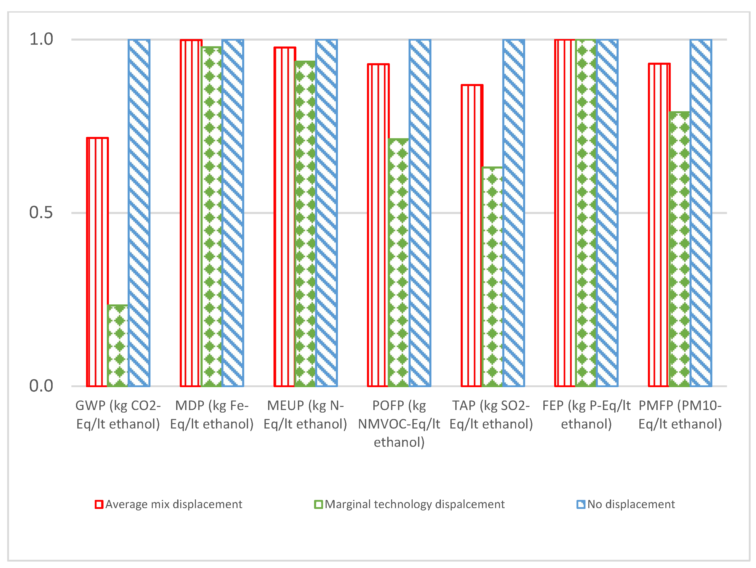
3.2. Impact Assessment of Ethanol Production

The seven impact categories results and the contribution analysis for each stage are shown in

Table 5. Impact categories in different stages to produce ethanol (FU = 1 L of ethanol).

Impact Category	Agricultural Stage		Milling Stage		Distillation Stage		Co-generation Stage		Total
	Impact Indicator Result	Contribution (%)	Impact Indicator Result	Contribution (%)	Impact Indicator Result	Contribution (%)	Impact Indicator Result	Contribution (%)	Impact Indicator Result
GWP (kg ${\mathrm{CO}}_{2\mathrm{eq}.}$)	0.28582	47.2	0.0013	0.2	0.369	60.9	−0.05059	−8.35	0.606
MDP (kg ${\mathrm{Fe}}_{\mathrm{eq}.}$)	0.00688	44.2	0.00089	5.7	0.0078	50.1	−0.0000048	−0.03	0.01557
MEUP (kg ${\mathrm{N}}_{\mathrm{eq}.}$)	0.0018	47.2	0.00001	0.3	0.00206459	54.2	−0.00006459	−1.70	0.00381
$\mathrm{POFP}(\mathrm{kg}{\mathrm{NMVOC}}_{\mathrm{eq}.}$)	0.00514	28	0.00249	13.6	0.01253	68.3	−0.00182	−9.92	0.01834
$\mathrm{TAP}(\mathrm{kg}{\mathrm{SO}}_{2\mathrm{eq}.}$)	0.00499	32.7	0.0012	7.9	0.0098	64.1	−0.00071	−4.65	0.01528
$\mathrm{FEP}(\mathrm{kg}{\mathrm{P}}_{\mathrm{eq}.}$)	0.0000928	34.4	0.0000372	13.8	0.00014	52	−0.00000031	−0.11	0.00027
PMFP (kg ${\mathrm{PM}}_{10\mathrm{eq}.}$)	0.00341	35.5	0.00083	8.1	0.00589	59	0.00006065	−0.60	0.01019

. The results shown in this subsection take into consideration the average mix displacement scenario, where the electricity produced in the co-generation power plant is displaced. The agricultural and distillation stages have the highest impacts in all categories.

The distillation stage has the highest contribution to GWP impact with 0.369 kg ${\mathrm{CO}}_2$ per liter of ethanol. Agriculture is the second system stage that contribute the most to the global warming potential impact (GWP) with 0.285 kg ${\mathrm{CO}}_2$ per liter of ethanol, followed by the milling stage with 0.0013 kg ${\mathrm{CO}}_2$ per liter of ethanol (Table 5). The co-generation stage reports a value of −0.0505 kg ${\mathrm{CO}}_2$ per liter of ethanol. This negative impact of the co-generation stage is mainly due to the fact that the emissions produced from the average mix include fossil-based power plants [78,84] and therefore there is a reduction in emissions from the displacement. The contribution of the distillation stage towards the GWP impact corresponds to ap-proximately 61%, followed by the agricultural stage with 47%, the milling stage with 0.2%, and the co-generation stage with −8.4%. The considerable contribution of the dis-tillation plant and the agricultural stage is mainly due to the emissions generated in the fermentation process and the urea and diesel used on field activities, respectively.

Freshwater eutrophication is measured in kilograms of phosphorous (kg of P) equivalents. The distillation and the agriculture stage have the most significant impact in this indicator with 0.0001 kg of P per liter of ethanol and 00000928 kof P per liter of ethanol, respectively (Table 5). The latter corresponds to 34% for the agricultural stage and 52% for the distillation stage of the overall impact. These results mainly due to the application of agrochemicals for sugarcane production and the high nitrogen and phosphorous content contained in the vinasse produced from the distillation column process.

Marine eutrophication is measured in kilograms of nitrogen (kg of N) equivalents. The ethanol life cycle shows that, overall, 0.00381 kg of ${\mathrm{N}}_{\mathrm{eq}.}$ are generated for each liter of ethanol produced. As can be seen, the distillation stage becomes the most important contributor in this impact category with 0.00206 kg of ${\mathrm{N}}_{\mathrm{eq}.}$/liter of ethanol, followed by the agricultural stage with 0.0018 kg of ${\mathrm{N}}_{\mathrm{eq}.}$/liter of ethanol, and by the milling stage with 0.00001 kg of ${\mathrm{N}}_{\mathrm{eq}.}$/liter of ethanol (Table 5). The co-generation stage reports a value of −0.000064 kg of ${\mathrm{N}}_{\mathrm{eq}.}$/liter of ethanol. Similar to the impact mentioned above (FEP), the distillation stage’s significant contribution (54%) is due to the high nitrogen content contained in the vinasse produced from the distillation column process. It is noteworthy that urea is used as a nitrogen source for the yeast production. The contribution percentage of the agricultural stage to this impact is 47% of the overall. The latter is mainly due to the agrochemicals application, such as nitrogenous fertilizers, for sugarcane production. The urea is a nitrogenous fertilizer that produces ammonium carbonate once it reacts with water, which then decomposes and releases ${\mathrm{NH}}_3$.

The metal depletion impact category assesses the scarcity of abiotic mineral resources and metals in terms of kg of iron ( ${\mathrm{Fe}}_{\mathrm{eq}.}$). Overall, 0.01557 kg ${\mathrm{Fe}}_{\mathrm{eq}.}$ per liter of ethanol are generated during the ethanol life cycle. Distillation is the system stage that contributes the most to MDP impact with 0.0078 kg ${\mathrm{Fe}}_{\mathrm{eq}.}$per liter of ethanol, followed by the agricultural stage with 0.0068 kg ${\mathrm{Fe}}_{\mathrm{eq}.}$ per liter of ethanol, the milling stage with 0.00089 kg ${\mathrm{Fe}}_{\mathrm{eq}.}$ per liter of ethanol, and the co-generation stage with −0.00000848 kg ${\mathrm{Fe}}_{\mathrm{eq}.}$per liter of ethanol (Table 5). The latter is mainly due to heavy metals that are incorporated through the use of fertilizers and pesticides. The contribution percentage of the agricultural, milling, distillation, and co-generation stages to this impact are 44%, 5.7%, 50%, and −0.031 of the overall, respectively.

The photochemical oxidant formation potential impact is measured in an equivalent value of kilograms of non-metal volatile organic compounds (kg ${\mathrm{NMVOC}}_{\mathrm{eq}.}$). The results for the ethanol life cycle are shown in kg ${\mathrm{NMVOC}}_{\mathrm{eq}.}$/liter of ethanol. The distillation stage becomes the most important contributor in this impact category with 0.012 kg ${\mathrm{NMVOC}}_{\mathrm{eq}.}$/liter of ethanol, followed by the agricultural stage with 0.0051 kg ${\mathrm{NMVOC}}_{\mathrm{eq}.}$/liter of ethanol and the milling stage with 0.0024 kg ${\mathrm{NMVOC}}_{\mathrm{eq}.}$/liter of ethanol (Table 5). The distillation stage has the most outstanding contribution with 68%. The agricultural stage has the second highest contribution with 28% due to the inappropriate chemical pesticides, which contain methane and halocarbon compounds [1]. The use of organic fertilizer helps reduce these pesticides that damage the environment [117]. The milling stage contributes to this impact with 12%. The co-generation stage has a contribution of −9.9%.

The particulate matter formation potential is measured in terms of kg of ${\mathrm{PM}}_{10\mathrm{eq}.}$. The ethanol life cycle shows that overall, 0.01019 kg of ${\mathrm{PM}}_{10\mathrm{eq}.}$are generated for each liter of ethanol produced. The distillation stage becomes the most important contributor in this impact category with 0.0058 kg of ${\mathrm{PM}}_{10\mathrm{eq}.}$/liter of ethanol, followed by the agricultural stage with 0.0034 kg of ${\mathrm{PM}}_{10\mathrm{eq}.}$/liter of ethanol and the milling stage with 0.00083 kg of ${\mathrm{PM}}_{10\mathrm{eq}.}$/liter of ethanol (Table 5). The contribution percentage of the agricultural, milling, and distillation stages to this impact are 33%, 8%, and 58% of the overall impact, respectively. The behavior of this environmental impact is mainly dominated by the emissions that are produced in the ethanol production chain, such as in the combustion of diesel in the agricultural stage, in bagasse burning to co-generate electricity and steam, or in the fermentation process within the distillation stage.

Terrestrial acidification potential is measured in kilograms of sulphur dioxide (kg of ${\mathrm{SO}}_2$) equivalents. The distillation and the agriculture stage have the most significant impact in this indicator with 0.0098 kg of ${\mathrm{SO}}_{2\mathrm{eq}.}$ per liter of ethanol and 0.0049 kg of ${\mathrm{SO}}_{2\mathrm{eq}.}$ per liter of ethanol, respectively (Table 5). The latter corresponds to 32% for the agricultural stage and 64% for the distillation stage of the overall impact. These results are mainly due to the application of agrochemicals for sugarcane production and the high nitrogen and phosphorous content contained in the vinasse produced from the distillation column process. The co-generation stage has a contribution of −4.6% of the overall impact due to the displacement of electricity.

3.2.1. Marginal Technology Displacement and No Displacement Scenarios

Figure 2 shows the environmental impacts for each scenario. The results obtained from each impact were normalized to a factor of 1 with the impact scores of the scenario “No displacement”. It is noteworthy that the scenario where the marginal electricity is displaced is the one that generates the lowest amount of environmental impacts. Fuel oil-based electricity is mainly displaced in the latter context. The most realistic scenario, the average mix displacement, occupies the second position in terms of the environmental impacts generated followed by the scenario where no surplus electricity displacement is considered. In the modelled system, ethanol has a better environmental performance when the electricity that is displacing has a lower environmental performance.

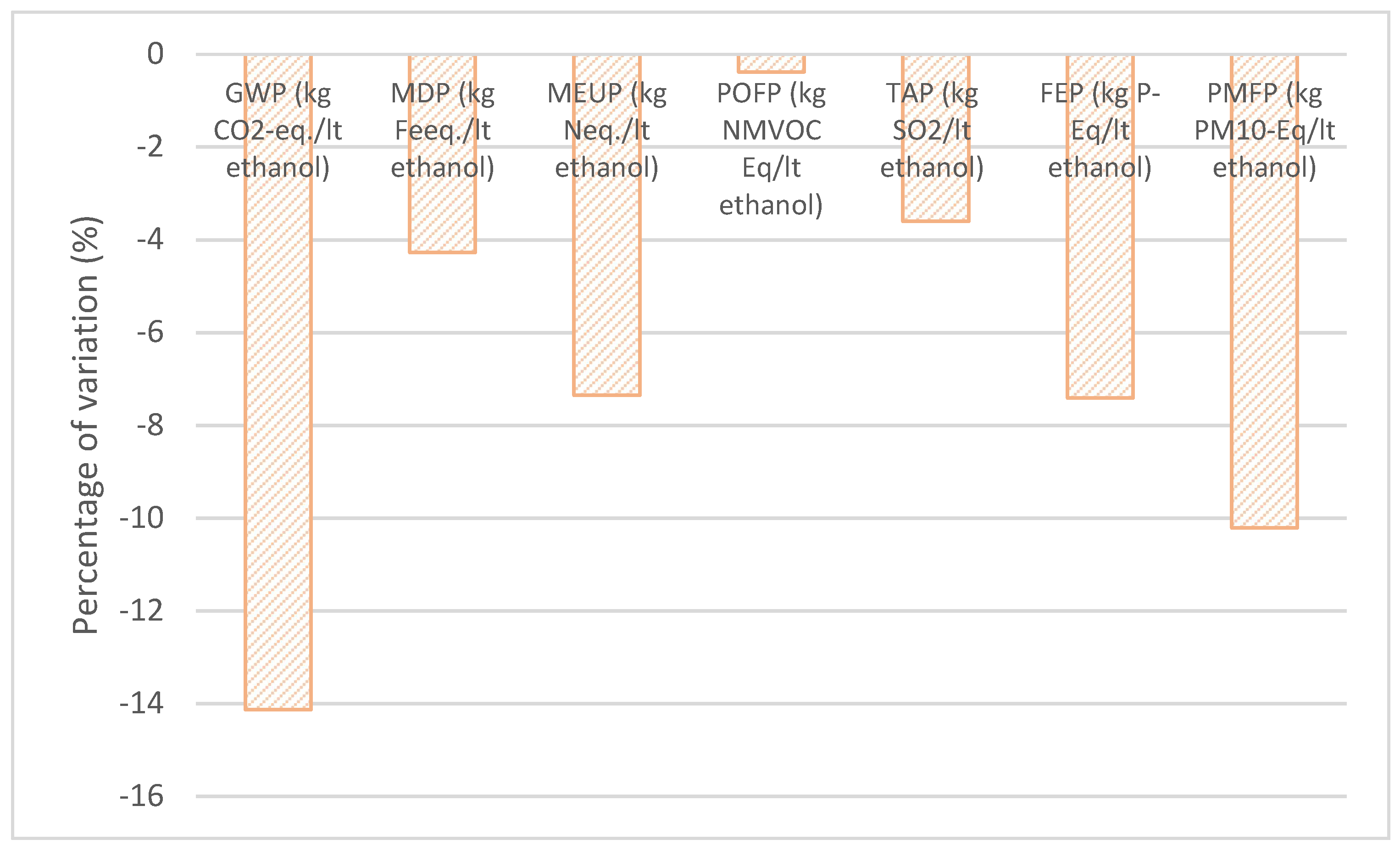
3.3. Sensitivity Analysis

The parameter considered for this sensitivity analysis is the productivity index. The impact category that has caught more attention is the global warming potential in order to see how sensitive it is in response to crop yield variation. This analysis shows that the global warming potential impact has a variation of −14% when the sugarcane productivity increases to 86 t/ha (Figure 3). The particulate matter formation potential impact also has a considerable decrease of 10% when the sugarcane yield increases from 71 to 86 t/ha.

4. Discussion

4.1. Comparison with Literature

The definition of system boundaries, functional units, allocation methods, technological conversion routes, and spatial and temporal variability differs widely among lifecycle analysis made of ethanol [10,40,118]. Furthermore, the sugarcane production system can be diversified with the different biorefineries configurations to obtain various products and by-products [60,119,120,121]. Only GWP impact results were compared with existing literature, as this is the impact indicator result that can be found in almost every study. Moreover, climate change is currently the main sustainability thread.

4.1.1. Comparison with Literature at the Sugarcane Production Level, at the Farm Gate

Environmental impacts are sensitive to ethanol conversion efficiency, sugarcane yield, and percentage of cane trash burn [60]. Based on the literature review, Watanabe et al. [111] reported a sugarcane yield of 82 tons per hectare (t/ha) for Brazil, compared to an average sugarcane yield of 78.15 t/ha for Indonesia [10]. On the other hand, Silalertruksa et al. [110], reported an average sugarcane yield of 75 t/ha for Thailand. The sugarcane yield of this study is lower than the compared articles and achieved a value of 70.9 t/ha in 2018 (

Table 6. GWP impact results at three different levels compared with the literature.

Ref.	Country	Yield	$\mathbf{C}{\mathbf{O}}_{2\mathbf{e}\mathbf{q}.}$			System Boundaries	Allocation	Bioethanol Generation
		(t/ha)	$\mathbf{kg}\mathbf{C}{\mathbf{O}}_{2\mathbf{e}\mathbf{q}.}/\mathbf{tc}$	$\mathbf{kg}\mathbf{C}{\mathbf{O}}_{2\mathbf{e}\mathbf{q}.}/\mathbf{ts}$	$\mathbf{kg}\mathbf{C}{\mathbf{O}}_{2\mathbf{e}\mathbf{q}.}/\mathbf{Liter}\mathbf{of}\mathbf{Ethanol}$
This study	Ecuador	70.9	53.6	568	0.60	Agricultural, milling, distillation, and co-generation stages	Economic	1G
[122] a	Brazil	87.1	-	-	0.44	Sugarcane production; processing; ethanol production	NA	1G
[122] b	Brazil	87.1	-	-	0.35	Sugarcane production; processing; ethanol production	NA	1G
[93]	Brazil	86.7	-	234	0.45	Sugarcane production; harvesting; transportation; processing; ethanol production; distribution	Economic, physical, and energy-based	1G
[112]	India	59.2	45	-	0.09–0.64 c	Sugarcane production; sugarcane processing to sugar; sugarcane processing to ethanol	Economic	2G
[123]	Brazil	-	-	-	0.35	Sugarcane production + local transport; ethanol production (without surplus energy credits)	NA	NA
[110]	Thailand	75	38	350	0.39	Sugarcane cultivation and harvesting, transportation; sugar milling, steam, and power generation from bagasse; molasses ethanol production, raw material production, and by-product utilization.	Economic allocation	2G
[113]	India	70	58.59	401	0.295	Sugarcane cultivation, co-generation, and ethanol production	Economic, mass and energy allocation	2G
[10]	Indonesia	78.1	49	-	0.61	Sugarcane harvesting, milling, ethanol production, and transport	Economic	2G

^a Scenario Brazil 2005, ^b Scenario Brazil 2020, ^c in ${\mathrm{CO}}_2$/kg of ethanol, tc: ton of sugarcane, ts: ton of sugar.

). The GWP impact from sugarcane production was reported as 53.6 kg of carbon-dioxide equivalent (kg ${\mathrm{CO}}_{2\mathrm{eq}.}$) per sugarcane ton. The main contributors of GWP impact at this level correspond to ${\mathrm{N}}_2\mathrm{O}$ lixiviation and volatilization, diesel used in agricultural machinery, and the urea production. Similar results of contribution analysis were stated by Tsiropoulos et al. [112], indicating that the GWP impact at the farm gate is mainly affected by the ${\mathrm{N}}_2\mathrm{O}$emissions from oxidation of nitrogen in nitrogenous fertilizers and by the emissions generated from their production.

The GWP impact of the study from India and Brazil show a lower value than the value reported in this study for sugarcane production with 45 and 36 kg ${\mathrm{CO}}_{2\mathrm{eq}.}$/ton of sugarcane, respectively [112]. The higher GWP impact in this study is mainly due to the greater amount of nitrogen and potassium fertilizers (3.95 kg/t and 0.92 kg/t, respectively) that are applied compared to the other studies (0.78–2.69 kg/t and 0.82–0.9 kg/t, respectively) [112].

A recent publication from Hiloidhari et al. [113] reported a carbon footprint of 58.59 kg ${\mathrm{CO}}_{2\mathrm{eq}.}$/t of sugarcane associated with the cultivation, transport, and processing stages (Table 6).

4.1.2. Comparison with Literature at the Ethanol Production Level at the Plant Gate

This study develops an environmental profile of ethanol produced through sugarcane in Ecuador, evaluating the effect using bagasse for the cogeneration of electricity. The GWP impact generated at the ethanol production level shows a value of 0.60 kg ${\mathrm{CO}}_{2\mathrm{eq}.}$/liter of ethanol based on Ecuadorian conditions and based on average mix displacement scenario (Table 6). This value falls within the range found in the literature 0.07–0.61 kg ${\mathrm{CO}}_{2\mathrm{eq}.}$/liter [10,93,110,112,113,122].

Tsiropoulos et al. [112] obtained a range of greenhouse gas emissions between 0.07 and 0.50 kg ${\mathrm{CO}}_{2\mathrm{eq}.}$/liter of ethanol in India for a high (surplus electricity accounted) and a low-system (no surplus electricity is accounted) performance, respectively. The low-system performance case of this latter study (0.50 kg ${\mathrm{CO}}_2$.liter of ethanol) has a lower carbon footprint than the average mix displacement scenario of our study (0.60 kg ${\mathrm{CO}}_{2\mathrm{eq}.}$/liter of ethanol). The ethanol from the latter study causes lower GHG emissions mainly because it is produced exclusively from molasses (2G), which is a by-product of sugar production. Moreover, the functional unit in the study by Tsiropoulos et al. [112] was defined as 1 kg of hydrous ethanol, compared to our study, which is 1 L of anhydrous ethanol. Nevertheless, for comparative purposes, the hydrous ethanol for our base scenario (average mix displacement) shows a GWP impact of 0.57 kg ${\mathrm{CO}}_{2\mathrm{eq}.}$/liter of ethanol. Additionally, the impact assessment was developed using Impact 2002+ methodology while this study used ReCiPe.

Compared to our study, Khatiwada et al. [10] reported a similar value of GWP (0.61 kg ${\mathrm{CO}}_{2\mathrm{eq}.}$/liter of ethanol) for ethanol production in Ionesia. The main difference between this latter study with our analysis is that the ethanol w produced basically with cane molasses pre-treated to obtain a concentrated juice before fermentation process. The authors also performed a sensitivity analysis of various pameters to evaluate energy and GHG balances in different allocation ratios. Similar to our study, the sensitivity analysis shows that the GHG emissions are highly sensitive to sugarcane yield. Pacheco et al. [124] reviewed that ethanol production can generate 0.35–0.40 kg ${\mathrm{CO}}_{2\mathrm{eq}.}$/liter of 1G ethanol through sugarcane feedstock in Brazil. On the other hand, Watanabe et al. [111] reported three different values of GWP impact based on three different biorefineries configurations: 0.447, 0.319, and 0.27 kg ${\mathrm{CO}}_{2\mathrm{eq}.}$/liter of ethanol for 1G-base, 1G-optimized, and integrated 1G2G ethanol biorefinery. Comparing our study with the 1G-optimized scenario, which represents a modern autonomous distillery for first-generation ethanol production and for electricity co-generation, there is a difference of 0.30 kg ${\mathrm{CO}}_{2\mathrm{eq}.}$/liter of ethanol. This difference could be related to the higher sugarcane yield (82 t/ha) of the study from Watanabe et al. [111] and also due to the sugarcane straw fraction recovered (50%) for energy generation in the cogeneration system.

Silalertruksa et al. [110] reported a GWP impact of 0.39 kg ${\mathrm{CO}}_{2\mathrm{eq}.}$/liter of molasses-derived-ethanol in Thailand, considering a base sugarcane biorefinery that includes conventional sugarcane farming, sugar milling, molasses ethanol production, and electricity generation. The lower GWP impact of this latter study compared with our study could be attributed to the higher sugarcane productivity (76 t/ha versus 71 t/ha) and the difference in sugar prices for the economic allocation (USD 27 versus USD 33 for a sack of 50 kg).

Finally, Hiloidhari et al. [113] assessed the life cycle ergy, carbon and water footprint of sugarcane based sugar, ethanol, and electricity in India. The GWP impact for ethanol production was reported as 0.29 kg ${\mathrm{CO}}_{2\mathrm{eq}.}$/liter of ethanol. The lower GWP impact for this latter study compared to our study could be atributed due to the fact that the ethanol in India is mainly produced from molasses (2G).

Regarding the system expansion applied in the co-generation stage, the marginal technology displacement and the no displacement scenarios report a GWP impact of 0.19 kg ${\mathrm{CO}}_{2\mathrm{eq}.}$/liter of ethanol and 0.84 kg ${\mathrm{CO}}_{2\mathrm{eq}.}$/liter of ethanol, respectively. The average mix displacement scenario was 0.60 kg ${\mathrm{CO}}_{2\mathrm{eq}.}$/liter of ethanol. The difference between the average and the marginal technology displacement scenarios is due to the credits of the Ecuadorian system, depending on what electricity is displaced. This difference is by a factor of 3.15. This factor is similar to what was reported by Tsiropoulos et al. [112], who compared an optimistic and a conservative surplus electricity system expansion scenario and estimated a difference factor of 3 [112]. Comparative results found in the literature indicate that the scenarios where system expansion is applied led to lower impact values compared to the scenario where no surplus electricity is displaced [24,112,125]. It is noteworthy that the carbon footprint of ethanol in systems that include co-generation depends on the mix or type of electricity displaced, as shown in Section 3.2.1.

Considering the contribution analysis, the results of the GWP impact at the plant gate indicate that sugarcane agricultural stage and the distillation stage have the highest contribution within the complete ethanol production chain with approximately 47% and 61%, respectively. These results are aligned with the results by Cavalett et al. [92] and Amores et al. [1], which concluded that the agricultural stage is one of the most intensive stages in terms of GHG emissions with 70% and a range of 58–63%, respectively. Amores et al., 2013 [1], states that the GWP impact is mainly affected by the fossil fuel utilization in the agricultural machinery. Gabisa et al. [102] also reported that the biggest contributor to GWP impact is sugarcane farming with a range contribution of 58.2–75%. In contrast, a study on molasses ethanol production in Indonesia showed that the agriculture stage has a contribution of 38% to the GWP impact releasing the other 62% of contribution to the industrial stages where the sugarcane is processed and then converted into ethanol [126].

4.2. Recommendations

The pilot program called Ecopais (95% extra gasoline with 5% anhydrous ethanol), which started in Guayaquil in 2010, sought the reduction of emissions to the environment and the reduction of oil derivative imports. The program has had positive environmental and social aspects. Nevertheless, the Ecuadorian sugarcane and ethanol industry should implement more efficient processes in its production chain to have the least possible environmental impact. Companies should apply industrial symbiosis and circular economy with the aim of fostering eco-innovation, creating and sharing mutually profitable transactions, and improving the business and technical processes of industries. Moreover, the bagasse should be used for electricity generation instead of considering it as an industrial waste.

Another recommendation should be focused on precision agriculture, specifically in the use of fertilizers. There are opportunities to reduce the amount of fertilizers used in the agriculture stage by implementing industrial symbiosis and circular economy strategies. Moreover, sugarcane growers must fertilize their agricultural fields in a coherent way to achieve precision in farming, guarantee greater sustainability, and maximize crop yield [114,115]. Another recommendation should be related to look for other agronomic alternatives to improve crop yield.

Aiming to achieve a higher percentage of ethanol in the mixture is necessary to invest in a more significant agricultural sugarcane expansion. Moreover, new technologies and conversion routes of biomass to explore the environmental benefits of other biofuels (2G and 3G) should be promoted. The integration of 1G and 2G technologies could reduce the GHG emissions of ethanol production by a factor of 1.4 compared to 1G technology [111].

4.3. Future Research Needs

Climate change impacts weather (rain events, temperatures), and alterations on sugarcane crop yield would be advisable to prospect the future security of supply of ethanol based on this crop. For example, if the sugarcane productivity drops to the Indian values (Table 6) of 59.2 ton/ha (a 16% decrease), the CO₂eq emissions per FU of our system would increase by 19%, maintaining all the other conditions. Droughts increase due to climate change, and contextualize the need to assess the water balance of the system. Water consumption can be categorized in blue, green, and gray. A water balance in terms of blue water entering the system and water vapor leaving the system to the atmosphere will be interesting to determine.

Improved yeast used in fermentation to increase ethanol production may have a positive impact on the systems, for example, an increase in ethanol yield of 20%, for the same conditions, would result in a mitigation of CO₂eq emissions per FU of 17%.

5. Conclusions

Biofuels have been recognized as an alternative transportation fuel to reduce fossil fuels consumption. Nevertheless, a detailed life cycle assessment is necessary to support its development. The environmental profile of ethanol derived from sugarcane was analyzed through a life cycle perspective including the effect of electricity co-generation in a sugar industrial complex. Four stages were considered for this analysis: agricultural, milling, distillation, and co-generation. The present study also compiles a life cycle inventory for ethanol-derived-sugarcane production in Ecuador.

The GWP impact generated at the farm gate level was reported as 53.6 kg of ${\mathrm{CO}}_{2\mathrm{eq}.}$ per sugarcane due to ${\mathrm{N}}_2\mathrm{O}$ volatilization and diesel application in agricultural machinery.

Considering the ethanol production level, the GWP impact was reported as 0.60 kg ${\mathrm{CO}}_{2\mathrm{eq}.}$/liter of ethanol. The contribution analysis shows that the agricultural stage and the ethanol distillation stage have the highest contribution on GWP impact within the complete ethanol production chain. Credits were received for displacing surplus electricity produced in the co-generation stage.

The terrestrial acidification potential impact was 0.01528 kg of ${\mathrm{SO}}_{2\mathrm{eq}.}$ at the ethanol production level due to the high nitrogen and phosphorous content in the vinasse. The marine eutrophication potential was calculated as 0.00381 kg of ${\mathrm{N}}_{\mathrm{eq}.}$ per 1 L of ethanol due to the high content of nitrogen contained in the vinasse and to the use of nitrogenous fertilizers in the agricultural stage.

The electricity demand covered by the industrial sugarcane sector reduces the demand for electricity generation by the power sector, and the ethanol life cycle is credited depending on whether it displaces average or marginal electricity. Three different scenarios were proposed in the co-generation stage: (i) average mix displacement scenario, where the surplus electricity produced in the co-generation stage is displaced; (ii) marginal technology displacement scenario, where the marginal surplus electricity is displaced from the mix, and (iii) no displacement scenario. The marginal technology displacement and the no displacement scenarios reports a GWP impact of 0.19 kg ${\mathrm{CO}}_{2\mathrm{eq}.}$/liter of ethanol and 0.84 kg ${\mathrm{CO}}_{2\mathrm{eq}.}$/liter of ethanol, respectively. The ethanol has a better environmental performance when the electricity that is displacing has a lower environmental performance.

The average mix displacement scenario reported a GWP impact of 0.60 kg ${\mathrm{CO}}_{2\mathrm{eq}.}$/liter of ethanol. Scenarios where system expansion is applied led to lower impact values compared to the scenario where no surplus electricity is displaced [125]. The latter shows the importance for the sugarcane industrial sector to increase its co-generation capacity in order to embrace its own electricity demand.

In order to have environmentally friendlier sugarcane and ethanol industries, sustainable and less polluting processes should be sought to reduce the environmental burdens. Companies should apply industrial symbiosis and circular economy strategies to produce lesser environmental loads within the ethanol production chain. Sugarcane growers must optimize synthetic fertilizers application by implementing precision agriculture to guarantee greater sustainability

Finally, Ecuador has mainly developed 1G ethanol derived from sugarcane through fermentation and distillation. There is a limited implementation of conversion processes of other feedstocks into ethanol in Ecuador, relegating the development of 2G and 3G biofuels. Therefore, future research should be focused on these biofuels.

This study contributes to the sustainability assessment of biofuel production, including the effect of electricity cogeneration from a sugar industry complex. Moreover, it allows the assessment of road transportation based on ethanol or ethanol and gasoline blends as fuels in Ecuador from a life cycle perspective.

References

1. Amores, M.J.; Mele, F.D.; Jiménez, L.; Castells, F. Life cycle assessment of fuel ethanol from sugarcane in Argentina. Int. J. Life Cycle Assess. 2013, 18, 1344–1357. [Google Scholar] [CrossRef]
2. Lisboa, C.C.; Butterbach-Bahl, K.; Mauder, M.; Kiese, R. Bioethanol production from sugarcane and emissions of greenhouse gases—known and unknowns. GCB Bioenergy 2011, 3, 277–292. [Google Scholar] [CrossRef]
3. Hanaki, K.; Portugal-Pereira, J. The Effect of Biofuel Production on Greenhouse Gas Emission Reductions. In Biofuels and Sustainability; Takeuchi, K., Shiroyama, H., Saito, O., Matsuura, M., Eds.; Springer: Tokyo, Japan, 2018; pp. 53–71. [Google Scholar]
4. REN21 Secretariat Market and Industry Trends. Available online: https://www.ren21.net/gsr-2019/chapters/chapter_03/chapter_03/ (accessed on 30 November 2021).
5. British Petroleum Company. BP Statistical Review of World Energy: June 2014; BP p.l.c.: London, UK, 2014. [Google Scholar]
6. Fargione, J.; Hill, J.; Tilman, D.; Polasky, S. Biofuels: Effects in landand fire—Response. Science 2008, 321, 199–200. [Google Scholar]
7. Ho, D.P.; Ngo, H.H.; Guo, W. A mini review on renewable sources for biofuel. Bioresour. Technol. 2014, 169, 742–749. [Google Scholar] [CrossRef] [PubMed] [Green Version]
8. Solomon, B.D. Biofuels and sustainability. Ann. N. Y. Acad. Sci. 2010, 1185, 119–134. [Google Scholar] [CrossRef] [PubMed]
9. Kates, R.W.; Clark, W.C.; Corell, R.; Hall, J.M.; Jaeger, C.C.; Lowe, I.; McCarthy, J.J.; Schellnhuber, H.J.; Bolin, B.; Dickson, N.M.; et al. Sustainability Science. Science 2001, 292, 641–642. [Google Scholar] [CrossRef]
10. Khatiwada, D.; Venkata, B.K.; Silveira, S.; Johnson, F.X. Energy and GHG balances of ethanol production from cane molasses in Indonesia. Appl. Energy 2016, 164, 756–768. [Google Scholar] [CrossRef]
11. Luque, R.; Herrero-Davila, L.; Campelo, J.M.; Clark, J.H.; Hidalgo, J.M.; Luna, D.; Marinas, J.M.; Romero, A.A. Biofuels: A technological perspective. Energy Environ. Sci. 2008, 1, 542–564. [Google Scholar] [CrossRef]
12. Ahorsu, R.; Medina, F.; Constantí, M. Significance and challenges of biomass as a suitable feedstock for bioenergy and biochemical production: A review. Energies 2018, 11, 3366. [Google Scholar] [CrossRef] [Green Version]
13. Food and Agriculture Organization of the United Nations (FAO). Biofuels: Prospects risks and opportunities. In The State of Food and Agriculture; FAO: Rome, Italy, 2008; pp. 1–97. [Google Scholar]
14. Lange, M. The GHG balance of biofuels taking into account land use change. Energy Policy 2011, 39, 2373–2385. [Google Scholar] [CrossRef] [Green Version]
15. Harchaoui, S.; Chatzimpiros, P. Energy, Nitrogen, and Farm Surplus Transitions in Agriculture from Historical Data Modeling. France, 1882–2013. J. Ind. Ecol. 2019, 23, 412–425. [Google Scholar] [CrossRef]
16. Sutton, M.A.; Bleeker, A.; Bekunda, M.; Grizzetti, B.; de Vries, W.; van Grinsven, H.J.M.; Abrol, Y.P.; Adhya, T.K.; Billen, G.; Davidson, E.A.; et al. Our Nutrient World: The Challenge to Produce More Food and Energy with Less Pollution; Centre for Ecology and Hydrology: Edinburgh, UK, 2013. [Google Scholar]
17. Levi, P.G.; Cullen, J.M. Mapping Global Flows of Chemicals: From Fossil Fuel Feedstocks to Chemical Products. Environ. Sci. Technol. 2018, 52, 1725–1734. [Google Scholar] [CrossRef] [PubMed]
18. Trimmer, J.T.; Guest, J.S. Recirculation of human-derived nutrients from cities to agriculture across six continents. Nat. Sustain. 2018, 1, 427–435. [Google Scholar] [CrossRef]
19. Koppelmäki, K.; Helenius, J.; Schulte, R.P.O. Nested circularity in food systems: A Nordic case study on connecting biomass, nutrient and energy flows from field scale to continent. Resour. Conserv. Recycl. 2021, 164, 105218. [Google Scholar] [CrossRef]
20. Miliotti, E.; Dell’Orco, S.; Lotti, G.; Rizzo, A.M.; Rosi, L.; Chiaramonti, D. Lignocellulosic ethanol biorefinery: Valorization of lignin-rich stream through hydrothermal liquefaction. Energies 2019, 12, 723. [Google Scholar] [CrossRef] [Green Version]
21. Pipitone, G.; Zoppi, G.; Frattini, A.; Bocchini, S.; Pirone, R.; Bensaid, S. Aqueous phase reforming of sugar-based biorefinery streams: From the simplicity of model compounds to the complexity of real feeds. Catal. Today 2020, 345, 267–279. [Google Scholar] [CrossRef]
22. Urbaniec, K.; Grabarczyk, R. Hydrogen production from sugar beet molasses—A techno-economic study. J. Clean. Prod. 2014, 65, 324–329. [Google Scholar] [CrossRef]
23. Guerra, J.P.M.; Coleta, J.R.; Arruda, L.C.M.; Silva, G.A.; Kulay, L. Comparative analysis of electricity cogeneration scenarios in sugarcane production by LCA. Int. J. Life Cycle Assess. 2014, 19, 814–825. [Google Scholar] [CrossRef] [Green Version]
24. Anne Renouf, M.; Pagan, R.J.; Wegener, M.K. Life cycle assessment of Australian sugarcane products with a focus on cane processing. Int. J. Life Cycle Assess. 2011, 16, 125–137. [Google Scholar] [CrossRef]
25. Arcentales, D.; Silva, C. Exploring the introduction of plug-in hybrid flex-fuel vehicles in Ecuador. Energies 2019, 12, 2244. [Google Scholar] [CrossRef] [Green Version]
26. ICAO. CORSIA Supporting Document: CORSIA Eligible Fuels—Life Cycle Assessment Methodology; ICAO: Montreal, QC, Canada, 2019. [Google Scholar]
27. European Union. Directive (EU) 2018/2001 of the European Parliament and of the Council of 11 December 2018 on the promotion of the use of energy from renewable sources. Off. J. Eur. Union 2018, 61, 82–209.
28. Paturau, J.M. By-Products of the Cane Sugar Industry—An Introduction to Their Industrial Utilization, 3rd ed.; Elsevier Publishing Company: Amsterdam, The Netherlands, 1989. [Google Scholar]
29. Miller, S.A.; Landis, A.E.; Theis, T.L. Environmental trade-offs of biobased production. Environ. Sci. Technol. 2007, 41, 5176–5182. [Google Scholar] [CrossRef] [Green Version]
30. von Blottnitz, H.; Curran, M.A. A review of assessments conducted on bio-ethanol as a transportation fuel from a net energy, greenhouse gas, and environmental life cycle perspective. J. Clean. Prod. 2007, 15, 607–619. [Google Scholar] [CrossRef]
31. Silva, C.; Pacheco, R.; Arcentales, D.; Santos, F. Sustainability of Sugarcane for Energy Purposes; Academic Press: Cambridge, MA, USA, 2019; ISBN 9780128142363. [Google Scholar]
32. Muralikrishna, I.V.; Manickam, V. Environmental Management Life Cycle Assessment. Environ. Manag. 2017, 1, 57–75. [Google Scholar]
33. Hill, J. Life Cycle Analysis of Biofuels. In Encyclopedia of Biodiversity: Second Edition; Elsevier Inc.: Amsterdam, The Netherlands, 2013; pp. 627–630. ISBN 9780123847195. [Google Scholar]
34. Sydney, E.B.; Letti, L.A.J.; Karp, S.G.; Sydney, A.C.N.; de Vandenberghe, L.P.S.; de Carvalho, J.C.; Woiciechowski, A.L.; Medeiros, A.B.P.; Soccol, V.T.; Soccol, C.R. Current analysis and future perspective of reduction in worldwide greenhouse gases emissions by using first and second generation bioethanol in the transportation sector. Bioresour. Technol. Rep. 2019, 7, 100234. [Google Scholar] [CrossRef]
35. Chum, H.L.; Warner, E.; Seabra, J.E.A.; Macedo, I.C. A comparison of commercial ethanol production systems from Brazilian sugarcane and US corn. Biofuels Bioprod. Biorefining 2014, 8, 205–223. [Google Scholar] [CrossRef]
36. Yan, X.; Corbin, K.R.; Burton, R.A.; Tan, D.K.Y. Agave: A promising feedstock for biofuels in the water-energy-food-environment (WEFE) nexus. J. Clean. Prod. 2020, 261, 121283. [Google Scholar] [CrossRef]
37. Pereira, L.G.; Cavalett, O.; Bonomi, A.; Zhang, Y.; Warner, E.; Chum, H.L. Comparison of biofuel life-cycle GHG emissions assessment tools: The case studies of ethanol produced from sugarcane, corn, and wheat. Renew. Sustain. Energy Rev. 2019, 110, 1–12. [Google Scholar] [CrossRef]
38. Stratton, R.W.; Wong, H.M.; Hileman, J.I. Quantifying variability in life cycle greenhouse gas inventories of alternative middle distillate transportation fuels. Environ. Sci. Technol. 2011, 45, 4637–4644. [Google Scholar] [CrossRef] [PubMed]
39. Farrell, A.E.; Plevin, R.J.; Turner, B.T.; Jones, A.D.; O’Hare, M.; Kammen, D.M. Ethanol can contribute to energy and environmental goals. Science 2006, 311, 506–508. [Google Scholar] [CrossRef] [PubMed] [Green Version]
40. Gnansounou, E.; Dauriat, A.; Villegas, J.; Panichelli, L. Life cycle assessment of biofuels: Energy and greenhouse gas balances. Bioresour. Technol. 2009, 100, 4919–4930. [Google Scholar] [CrossRef] [PubMed]
41. Beer, T.; Grant, T. Life-cycle analysis of emissions from fuel ethanol and blends in Australian heavy and light vehicles. J. Clean. Prod. 2007, 15, 833–837. [Google Scholar] [CrossRef]
42. Wallace, J.; Wang, M.; Weber, T.; Finizza, A. Well-to-wheel analysis of energy use and greenhouse gas emissions of advanced fuel/vehicle systems—North American analysis Volume 3. GM Study Well-to-Wheel Energy Use Greenh. Gas Emiss. Adv. Fuel/Vehicle Syst. 2001, 3, 1–41. [Google Scholar]
43. Kim, S.; Dale, B.E. Life cycle assessment of fuel ethanol derived from corn grain via dry milling. Bioresour. Technol. 2008, 99, 5250–5260. [Google Scholar] [CrossRef]
44. Malça, J.; Freire, F. Renewability and life-cycle energy efficiency of bioethanol and bio-ethyl tertiary butyl ether (bioETBE): Assessing the implications of allocation. Energy 2006, 31, 3362–3380. [Google Scholar] [CrossRef] [Green Version]
45. Shapouri, H.; Duffield, J.A.; Wang, M. The Energy Balance of Corn Ethanol Revisited. Trans. Am. Soc. Agric. Eng. 2003, 46, 959–968. [Google Scholar] [CrossRef]
46. Elsayed, M.A.; Matthews, R.; Mortimer, N.D. Carbon and Energy Balances for a Range of Biofuels Options; Sheffield Hallam University: Sheffield, UK, 2003. [Google Scholar]
47. Isaias de Carvalho Macedo. Assessment of Greenhouse Gas Emissions in the Production and Use of Fuel Ethanol in Brazil; Government of the State of Sao Paulo: Sao Paulo, Brazil, 2003. [Google Scholar]
48. Luo, L.; van der Voet, E.; Huppes, G. Life cycle assessment and life cycle costing of bioethanol from sugarcane in Brazil. Renew. Sustain. Energy Rev. 2009, 13, 1613–1619. [Google Scholar] [CrossRef]
49. Bai, Y.; Luo, L.; Van Der Voet, E. Life cycle assessment of switchgrass-derived ethanol as transport fuel. Int. J. Life Cycle Assess. 2010, 15, 468–477. [Google Scholar] [CrossRef] [Green Version]
50. Roberto Ometto, A.; Zwicky Hauschild, M.; Nelson Lopes Roma, W. Lifecycle assessment of fuel ethanol from sugarcane in Brazil. Int. J. Life Cycle Assess. 2009, 14, 236–247. [Google Scholar] [CrossRef]
51. Renouf, M.A.; Wegener, M.K.; Pagan, R.J. Life cycle assessment of Australian sugarcane production with a focus on sugarcane growing. Int. J. Life Cycle Assess. 2010, 15, 927–937. [Google Scholar] [CrossRef]
52. Botha, T.; von Blottnitz, H. A comparison of the environmental benefits of bagasse-derived electricity and fuel ethanol on a life-cycle basis. Energy Policy 2006, 34, 2654–2661. [Google Scholar] [CrossRef]
53. Cherubini, F.; Ulgiati, S. Crop residues as raw materials for biorefinery systems—A LCA case study. Appl. Energy 2010, 87, 47–57. [Google Scholar] [CrossRef]
54. IEA. Energy Technology Perspective. Scenario and Strategies to 2050; The Otganisation for Economic Cooperation and Development: Paris, France, 2008. [Google Scholar]
55. Saladini, F.; Patrizi, N.; Pulselli, F.M.; Marchettini, N.; Bastianoni, S. Guidelines for emergy evaluation of first, second and third generation biofuels. Renew. Sustain. Energy Rev. 2016, 66, 221–227. [Google Scholar] [CrossRef]
56. Sendelius, J. Steam Pretreatment Optimisation for Sugarcane Bagasse in Bioethanol Production. Master’s Thesis, Lund University, Lund, Sweden, 2005. [Google Scholar]
57. Quintero, J.A.; Montoya, M.I.; Sánchez, O.J.; Giraldo, O.H.; Cardona, C.A. Fuel ethanol production from sugarcane and corn: Comparative analysis for a Colombian case. Energy 2008, 33, 385–399. [Google Scholar] [CrossRef]
58. Morales, M.; Quintero, J.; Conejeros, R.; Aroca, G. Life cycle assessment of lignocellulosic bioethanol: Environmental impacts and energy balance. Renew. Sustain. Energy Rev. 2015, 42, 1349–1361. [Google Scholar] [CrossRef]
59. Nguyen, T.L.T.; Gheewala, S.H. Life cycle assessment of fuel ethanol from cane molasses in Thailand. Int. J. Life Cycle Assess. 2008, 13, 301. [Google Scholar] [CrossRef]
60. Silalertruksa, T.; Gheewala, S.H. Environmental sustainability assessment of bio-ethanol production in Thailand. Energy 2009, 34, 1933–1946. [Google Scholar] [CrossRef]
61. Halleux, H.; Lassaux, S.; Renzoni, R.; Germain, A. Comparative life cycle assessment of two biofuels: Ethanol from sugar beet and rapeseed methyl ester. Int. J. Life Cycle Assess. 2008, 13, 184. [Google Scholar] [CrossRef]
62. Shapouri, H. TheEnergy Balance of Corn Ethanol Revisited. Trans. ASAE 2003, 46, 959–968. [Google Scholar] [CrossRef]
63. Wang, M.; Wu, M.; Huo, H.; Liu, J. Life-cycle energy use and greenhouse gas emission implications of Brazilian sugarcane ethanol simulated with the GREET model. Int. Sugar J. 2008, 110, 1–15. [Google Scholar]
64. Hoefnagels, R.; Smeets, E.; Faaij, A. Greenhouse gas footprints of different biofuel production systems. Renew. Sustain. Energy Rev. 2010, 14, 1661–1694. [Google Scholar] [CrossRef]
65. Faaij, A.P.C. Bio-energy in Europe: Changing technology choices. Energy Policy 2006, 34, 322–342. [Google Scholar] [CrossRef] [Green Version]
66. Cardona, C.A.; Quintero, J.A.; Paz, I.C. Production of bioethanol from sugarcane bagasse: Status and perspectives. Bioresour. Technol. 2010, 101, 4754–4766. [Google Scholar] [CrossRef]
67. Kadam, K.L. Environmental benefits on a life cycle basis of using bagasse-derived ethanol as a gasoline oxygenate in India. Energy Policy 2002, 30, 371–384. [Google Scholar] [CrossRef]
68. Sheehan, J.; Aden, A.; Paustian, K.; Killian, K.; Brenner, J.; Walsh, M.; Nelson, R. Energy and environmental aspects of using corn stover for fuel ethanol. J. Ind. Ecol. 2003, 7, 117–146. [Google Scholar] [CrossRef]
69. Spatari, S.; Zhang, Y.; Maclean, H.L. Life cycle assessment of switchgrass- and corn stover-derived ethanol-fueled automobiles. Environ. Sci. Technol. 2005, 39, 9750–9758. [Google Scholar] [CrossRef] [PubMed]
70. Wu, M.; Wang, M.; Huo, H. Fuel-Cycle Assessment of Selected Bioethanol Production Pathways in the United States; Argonne National Laboratory: Lemont, IL, USA, 2006. [Google Scholar]
71. Khatiwada, D.; Silveira, S. Net energy balance of molasses based ethanol: The case of Nepal. Renew. Sustain. Energy Rev. 2009, 13, 2515–2525. [Google Scholar] [CrossRef]
72. Gopal, A.R.; Kammen, D.M. Molasses for ethanol: The economic and environmental impacts of a new pathway for the lifecycle greenhouse gas analysis of sugarcane ethanol. Environ. Res. Lett. 2009, 4, 044005. [Google Scholar] [CrossRef]
73. Medina, S. Atlas Bioenergético de la República del Ecuador; Ministerio de Electricidad y Energía Renovable; e, Instituto Nacional de Preinversión: Pichincha, Ecuador, 2014. [Google Scholar]
74. Chiriboga, G.; De La Rosa, A.; Molina, C.; Velarde, S.; Carvajal C, G. Energy Return on Investment (EROI) and Life Cycle Analysis (LCA) of biofuels in Ecuador. Heliyon 2020, 6, e04213. [Google Scholar] [CrossRef]
75. Ministerio Coordinador de Sectores Estratégicos. Agenda Nacional de Energía 2016–2040; Ministerio Coordinador de Sectores Estratégicos: Quito, Ecuador, 2017. [Google Scholar]
76. EP Petroecuador. Empresa Pública de Hidrocarburos del Ecuador Plan Estratégico Empresarial 2018–2021; EP Petroecuador: Quito, Ecuador, 2020. [Google Scholar]
77. Briones-Hidrovo, A.; Uche, J.; Martínez-Gracia, A. Determining the net environmental performance of hydropower: A new methodological approach by combining life cycle and ecosystem services assessment. Sci. Total Environ. 2020, 712, 136369. [Google Scholar] [CrossRef]
78. Ramirez, A.D.; Boero, A.; Rivela, B.; Melendres, A.M.; Espinoza, S.; Salas, D.A. Life cycle methods to analyze the environmental sustainability of electricity generation in Ecuador: Is decarbonization the right path? Renew. Sustain. Energy Rev. 2020, 134, 110373. [Google Scholar] [CrossRef]
79. Briones Hidrovo, A.; Uche, J.; Martínez-Gracia, A. Accounting for GHG net reservoir emissions of hydropower in Ecuador. Renew. Energy 2017, 112, 209–221. [Google Scholar] [CrossRef] [Green Version]
80. Porras, F.; Ramirez, A.D.; Walter, A.; Soriano, G. Life cycle assessment of greenhouse gas emissions: Comparison between a cooling tower and a geothermal heat exchanger for air conditioning applications in Ecuador. In Proceedings of the ASME 2019 13th International Conference on Energy Sustainability, ES 2019, collocated with the ASME 2019 Heat Transfer Summer Conference, Bellevue, WA, USA, 14–17 July 2019. [Google Scholar]
81. Ramirez, A.D.; Perez, E.F.; Boero, A.J.; Salas, D.A. Carbon footprint of energy systems: Liquefied petroleum gas based cooking vs electricity based cooking in Ecuador. In Proceedings of the ASME International Mechanical Engineering Congress and Exposition, Tampa, FL, USA, 3–9 November 2017; Volume 6. [Google Scholar]
82. Ramirez, A.D.; Arcentales, D.; Boero, A. Mitigation of greenhouse gas emissions through the shift from fossil fuels to electricity in the mass transport system in guayaquil, ecuador. In Proceedings of the ASME International Mechanical Engineering Congress and Exposition, Pittsburgh, PA, USA, 9–15 November 2018; A-144113. Volume 6. [Google Scholar]
83. Parra, C.R.; Corrêa-Guimarães, A.; Navas-Gracia, L.M.; Narváez, C., R. Bioenergy on islands: An environmental comparison of continental palm oil vs. local waste cooking oil for electricity generation. 2020, 10, 3806. [Google Scholar] [CrossRef]
84. Ramirez, A.D.; Rivela, B.; Boero, A.; Melendres, A.M. Lights and shadows of the environmental impacts of fossil-based electricity generation technologies: A contribution based on the Ecuadorian experience. Energy Policy 2019, 125, 467–477. [Google Scholar] [CrossRef]
85. Muñoz Mayorga, M.; Herrera Orozco, I.; Lechón Pérez, Y.; Caldés Gomez, N.; Iglesias Martínez, E. Environmental Assessment of Electricity Based on Straight Jatropha Oil on Floreana Island, Ecuador. Bioenergy Res. 2018, 11, 123–138. [Google Scholar] [CrossRef]
86. Guerrero, A.B.; Muñoz, E. Life cycle assessment of second generation ethanol derived from banana agricultural waste: Environmental impacts and energy balance. J. Clean. Prod. 2018, 174, 710–717. [Google Scholar] [CrossRef]
87. Graefe, S.; Dufour, D.; Giraldo, A.; Muñoz, L.A.; Mora, P.; Solís, H.; Garcés, H.; Gonzalez, A. Energy and carbon footprints of ethanol production using banana and cooking banana discard: A case study from Costa Rica and Ecuador. Biomass Bioenergy 2011, 35, 2640–2649. [Google Scholar] [CrossRef]
88. National Energy Technology Laboratory. Development of Baseline Data and Analysis of Life Cycle Greenhouse Gas Emissions of Petroleum-Based Fuels; National Energy Technology Laboratory: Pittsburgh, PA, USA, 2008. [Google Scholar]
89. RSB—Roundtable on Sustainable Biomaterials. RSB Fossil Fuel Baseline Calculation Methodology; RSB: Geneva, Switzerland, 2011. [Google Scholar]
90. ISO 14044:2006; Environmental Management—Life Cycle Assessment—Requirements and Guidelines. International Organization for Standardization: Geneva, Switzerland, 2006.
91. ISO 14040:2006; International Standard. Environmental management—Life Cycle Assessment—Principles and Framework. International Organization for Standardization: Geneva, Switzerland, 2006.
92. Cavalett, O.; Junqueira, T.L.; Dias, M.O.S.; Jesus, C.D.F.; Mantelatto, P.E.; Cunha, M.P.; Franco, H.C.J.; Cardoso, T.F.; Filho, R.M.; Rossell, C.E.V.; et al. Environmental and economic assessment of sugarcane first generation biorefineries in Brazil. Clean Technol. Environ. Policy 2012, 14, 399–410. [Google Scholar] [CrossRef]
93. Seabra, J.E.A.; Macedo, I.C.; Chum, H.L.; Faroni, C.E.; Sarto, C.A. Life cycle assessment of Brazilian sugarcane products: GHG emissions and energy use. Biofuels Bioprod. Biorefining 2011, 5, 519–532. [Google Scholar] [CrossRef]
94. Ekvall, T.; Weidema, B.P. System boundaries and input data in consequential life cycle inventory analysis. Int. J. Life Cycle Assess. 2004, 9, 161–171. [Google Scholar] [CrossRef]
95. Arconel. Estadística Anual y Multianual del Sector Eléctrico Ecuatoriano. BMC Public Health 2017, 5, 1–149. [Google Scholar]
96. LOSPEE Reglamento General de la Ley Orgánica del Servicio Público de Energía Eléctrica. Regist. Of. Año I—No 21; Asamblea Nacional de la República del Ecuador: Quito, Ecuador, 2019.
97. Nemecek, T.; Kagi, T. Life Cycle Inventories of Swiss and European Agricultural Production Systems, Ecoinvent Report No. 15; Swiss Centre for Life Cycle Inventories: Zurich, Switzerland, 2007. [Google Scholar]
98. Ecoinvent v3.4 Ecoinvent Database—Ecoinvent. Available online: https://ecoinvent.org/the-ecoinvent-database/ (accessed on 30 September 2021).
99. IPCC, I.P.O.C.C. Climate Change 2007—The Physical Science Basis: Working Group I Contribution to the Fourth Assessment Report of the IPCC; Cambridge University Press: Cambridge, UK, 2007. [Google Scholar]
100. Ministérioda Ciência e Tecnologia—MCT. Primeiro Inventário Brasileiro de Emissões Antrópicas de Gases de Efeito Estufa; Ministérioda Ciência e Tecnologia: Sao Paulo, Brazil, 2011. [Google Scholar]
101. IPCC. Chapter 11: N2O emissions from managed soils, and CO2 emissions from lime and urea application. In 2019 Refinement to the 2006 IPCC Guidelines for National Greenhouse Gas Inventories; Intergovernmental Panel on Climate Change: Geneva, Switzerland, 2019; Volume 4. [Google Scholar]
102. Gabisa, E.W.; Bessou, C.; Gheewala, S.H. Life cycle environmental performance and energy balance of ethanol production based on sugarcane molasses in Ethiopia. J. Clean. Prod. 2019, 234, 43–53. [Google Scholar] [CrossRef]
103. Diario El Universo Producción de caña de azúcar y etanol genera 200.000 plazas de trabajo, según la Asociación de Biocombustibles del Ecuador. Editorial Diario El Universo, Ecuador. 2021. Available online: https://www.google.com.hk/url?sa=t&rct=j&q=&esrc=s&source=web&cd=&ved=2ahUKEwjZ_vm_gpH5AhUDq1YBHS-zB70QFnoECAoQAQ&url=https%3A%2F%2Fwww.eluniverso.com%2Fnoticias%2Feconomia%2Fproduccion-de-cana-de-azucar-y-etanol-genera-200000-plazas-de-trabajo-segun-la-asociacion-de-biocombustibles-del-ecuador-nota%2F&usg=AOvVaw1L4GleS27OhwiQaO7d0DJR (accessed on 30 June 2022).
104. Birru, E. Sugar Cane Industry Overview And Energy Efficiency Considerations; KTH Royal Institute of Technology: Stockholm, Sweden, 2016. [Google Scholar]
105. ARCONEL. Estadísticas del Sector Eléctrico Ecuatoriano; ARCONEL: Quito, Ecuador, 2015. [Google Scholar]
106. PME Plan Maestro de Electricidad 2016–2025; Ministerio de Electricidad y Energía Renovable, Equipo Técnico Interinstitucional: Quito, Ecuador, 2017.
107. Graesser, J.; Aide, T.M.; Grau, H.R.; Ramankutty, N. Cropland/pastureland dynamics and the slowdown of deforestation in Latin America. Environ. Res. Lett. 2015, 10, 034017. [Google Scholar] [CrossRef]
108. Nagy, R.C.; Porder, S.; Brando, P.; Davidson, E.A.; Figueira, A.M.E.S.; Neill, C.; Riskin, S.; Trumbore, S. Soil Carbon Dynamics in Soybean Cropland and Forests in Mato Grosso, Brazil. J. Geophys. Res. Biogeosci. 2018, 123, 18–31. [Google Scholar] [CrossRef] [PubMed] [Green Version]
109. Spawn, S.A.; Lark, T.J.; Gibbs, H.K. Carbon emissions from cropland expansion in the United States. Environ. Res. Lett. 2019, 14, 045009. [Google Scholar] [CrossRef]
110. Silalertruksa, T.; Gheewala, S.H.; Pongpat, P. Sustainability assessment of sugarcane biorefinery and molasses ethanol production in Thailand using eco-efficiency indicator. Appl. Energy 2015, 160, 603–609. [Google Scholar] [CrossRef]
111. Watanabe, M.D.B.; Chagas, M.F.; Cavalett, O.; Guilhoto, J.J.M.; Griffin, W.M.; Cunha, M.P.; Bonomi, A. Hybrid Input-Output Life Cycle Assessment of First- and Second-Generation Ethanol Production Technologies in Brazil. J. Ind. Ecol. 2016, 20, 764–774. [Google Scholar] [CrossRef]
112. Tsiropoulos, I.; Faaij, A.P.C.; Seabra, J.E.A.; Lundquist, L.; Schenker, U.; Briois, J.F.; Patel, M.K. Life cycle assessment of sugarcane ethanol production in India in comparison to Brazil. Int. J. Life Cycle Assess. 2014, 19, 1049–1067. [Google Scholar] [CrossRef]
113. Hiloidhari, M.; Haran, S.; Banerjee, R.; Rao, A.B. Life cycle energy–carbon–water footprints of sugar, ethanol and electricity from sugarcane. Bioresour. Technol. 2021, 330, 125012. [Google Scholar] [CrossRef] [PubMed]
114. Ramamurthy, V.; Naidu, L.G.K.; Ramesh Kumar, S.C.; Srinivas, S.; Hegde, R. Soil-based fertilizer recommendations for precision farming. Curr. Sci. 2009, 97, 641–647. [Google Scholar]
115. Sanches, G.M.; de Paula, M.T.N.; Magalhães, P.S.G.; Duft, D.G.; Vitti, A.C.; Kolln, O.T.; Borges, B.M.M.N.; Franco, H.C.J. Precision production environments for sugarcane fields. Sci. Agric. 2019, 76, 10. [Google Scholar] [CrossRef] [Green Version]
116. Tubiello, F.; Cóndor-Golec, R.; Salvatore, M.; Piersante, A.; Federici, S.; Ferrara, A.; Rossi, S.; Flammini, A.; Cardenas, P.; Biancalani, R.; et al. Estimación de Emisiones de Gases de Efecto Invernadero en la Agricultura. Un Manual Para Abordar Los Requisitos de Los Datos Para Los Países en Desarrollo; FAO: Rome, Italy, 2015. [Google Scholar]
117. El-Haggar, S.M. Sustainability of Agricultural and Rural Waste Management; Academic Press: Cambridge, MA, USA, 2007. [Google Scholar]
118. Stichnothe, H.; Azapagic, A. Bioethanol from waste: Life cycle estimation of the greenhouse gas saving potential. Resour. Conserv. Recycl. 2009, 53, 624–630. [Google Scholar] [CrossRef]
119. Dias, M.O.S.; Junqueira, T.L.; Cavalett, O.; Cunha, M.P.; Jesus, C.D.F.; Rossell, C.E.V.; Maciel Filho, R.; Bonomi, A. Integrated versus stand-alone second generation ethanol production from sugarcane bagasse and trash. Bioresour. Technol. 2012, 103, 152–161. [Google Scholar] [CrossRef] [PubMed] [Green Version]
120. Dias, M.O.S.; Junqueira, T.L.; Cavalett, O.; Pavanello, L.G.; Cunha, M.P.; Jesus, C.D.F.; Maciel Filho, R.; Bonomi, A. Biorefineries for the production of first and second generation ethanol and electricity from sugarcane. Appl. Energy 2013, 109, 72–78. [Google Scholar] [CrossRef]
121. Wang, L.; Quiceno, R.; Price, C.; Malpas, R.; Woods, J. Economic and GHG emissions analyses for sugarcane ethanol in Brazil: Looking forward. Renew. Sustain. Energy Rev. 2014, 40, 571–582. [Google Scholar] [CrossRef]
122. Macedo, I.C.; Seabra, J.E.A.; Silva, J.E.A.R. Green house gases emissions in the production and use of ethanol from sugarcane in Brazil: The 2005/2006 averages and a prediction for 2020. Biomass Bioenergy 2008, 32, 582–595. [Google Scholar] [CrossRef]
123. Edwards, R.; Hass, H.; Larivé, J.-F.; Lonza, L.; Mass, H.; Rickeard, D.; Larive, J.-F.; Rickeard, D.; Weindorf, W. Well-to-Wheels analysis of future automotive fuels and powertrains in the European context Report. Jt. Res. Cent. EU Ispra Italy 2013, 4, 1–62. [Google Scholar]
124. Pacheco, R.; Silva, C. Global warming potential of biomass-to-ethanol: Review and sensitivity analysis through a case study. Energies 2019, 12, 2535. [Google Scholar] [CrossRef] [Green Version]
125. Murali, G.; Shastri, Y. Life-cycle assessment-based comparison of different lignocellulosic ethanol production routes. Biofuels 2022, 13, 237–247. [Google Scholar] [CrossRef]
126. Silveira, S.; Khatiwada, D. Ethanol production and fuel substitution in Nepal-Opportunity to promote sustainable development and climate change mitigation. Renew. Sustain. Energy Rev. 2010, 14, 1644–1652. [Google Scholar] [CrossRef]
Figure 1. Anhydrous ethanol life cycle system boundaries and main product flows quantification for year 2018.
Energies 15 05421 g001
Figure 2. Comparison of life cycle environmental impacts at cradle-to-plant-gate for the three different system expansion scenarios: Average mix displacement, marginal technology displacement and no displacement. The impact results were normalized to a factor of 1 according to the impact category result indicator of the scenario “No displacement”.
Energies 15 05421 g002
Figure 3. Percentage of variation for each environmental impact indicator result through an increase of crop yield from 71 to 86 t/ha.
Energies 15 05421 g003