Power and Flow Analysis of Axial Induction Control in an Array of Model-Scale Wind Turbines

Abstract

As research on wind energy has progressed, it has broadened from a focus on the wind turbine to include the entire wind farm. In particular, methods to mitigate the negative effects of upstream wakes on downstream turbines have received significant attention. One such mitigation method is axial induction control (AIC) in which upstream turbines are derated to reduce the momentum deficits in their wakes, leaving higher speed flow for downstream turbines. If performed correctly, it is theorized that the power production gains in downstream turbines can compensate for the power sacrificed by derating upstream turbines. Previous work has indicated that the “excess” energy left in the wake of the derated turbine is along the edges of the wake such that a turbine placed directly downstream will see little to no increase in power. To address this hypothesis, we performed a control and treatment experiment with model-scale turbines in a wide flume. Five turbines were arranged in three successive streamwise rows, with the first two rows consisting of two aligned turbines, while three turbines with small transverse spacing were placed in the third row, the central of which was also streamwise-aligned with the upstream two turbines. This arrangement was used to evaluate the difference in power production primarily among the turbines in the third row when the upstream turbines were derated. Particle image velocimetry (PIV) was used to measure the wake in the streamwise-vertical planes along the centerline of the array and along the rotor tips of the centerline turbines between all rows, and high accuracy power measurements were recorded from each turbine. The results show that the total power of the array was decreased while implementing AIC but that individual turbine performance differed from predictions. PIV results show that mean kinetic energy (MKE) is redistributed to the edges of the wakes as has been previously hypothesized. We provide an analysis of the results that connects both the power and flow measurements and that highlights several of the aspects of wind turbine wake flows that make them so complex and challenging to study.

1. Introduction

Windmills date back to at least the ninth century [1], but the wind turbine in its modern form is a relatively young technology. Wind farms are even newer. Historically, most optimization efforts have focused on individual wind turbines, and only in the last decade or two have there been significant efforts to optimize wind farms. Because of this, the starting point for wind farm design was that optimized turbines would lead to optimized wind farms as long as sufficient spacing was provided for wake decay between turbines. While there is some truth to this, the complicated fluid dynamics of a boundary layer flow through a wind farm, as well as economic factors, have led to new insights regarding best practices for energy harvesting maximization and structural load reduction when optimizing wind farms. The new approach is holistic and seeks to optimize the farm and not the turbines. There are several proposed methods to do this [2,3], some of which focus on power maximization, others on structural load reduction, while some may fulfill both of these objectives.

The following study is focused on static axial induction control (AIC), which was introduced as early as 1988 by ref. [4]. As mentioned above, the conventional approach for wind farm operation stems from the idea that optimally operated turbines will lead to an optimally operated wind farm. In this approach, each turbine, agnostic of the other turbines in the wind farm, uses information from sensors in the turbine as inputs to a feedback loop that, barring extreme conditions, will seek to maximize its power production. In AIC, the operating point of each turbine (how much power it produces and therefore how much energy it extracts from the flow) is set such that the interactions of turbines and flow optimize the total power produced by the wind farm, though with AIC, some turbines may not be optimally operated when considered individually. Just as in conventional operation, the exact operating points for AIC are likely to depend on the flow conditions (wind speed, direction, turbulence level, and boundary layer stability), and the turbines are still agnostic to one another. Instead, AIC requires previous knowledge, likely gained through testing and previous studies, to establish the optimal operating points for the given conditions [5,6].

Reviews of AIC and other power maximization techniques are given by refs. [2,3]. Most prior work indicates that the optimal implementation of AIC would have turbine power production increase with downstream placement within the farm such that the last row operates optimally as individual turbines [7,8], though it quickly becomes more complex when considering irregular wind farm layouts and multiple wind directions and speeds. Taking the simplest case of two wind turbines aligned with the flow, there is an inverse relationship between the power production of the upstream turbine and its negative wake effects on the power production of the downstream turbine. In theory, some operating point for the upstream turbine that is less than its individual optimum will maximize the sum of power produced by both turbines. This assumes that the two turbines are not sufficiently far enough apart that the downstream turbine is unaffected by the wake of the upstream turbine. This is because derating the upstream turbine reduces the momentum deficit it creates, which leaves higher velocity flow for the downstream turbine, thereby increasing its power production. That most downstream turbines should be operated at their individual optima may be intuitively obvious as only the most downstream turbines do not subject other turbines to their wakes, so they should operate optimally and extract as much energy from the wind as possible.

There is, however, uncertainty regarding the best way to derate an upstream turbine. In particular, a turbine can produce less power while producing more or less thrust depending on the way in which it is derated [9,10]. Ref. [9] summarizes the situation well by pointing out that an increase (decrease) in thrust is likely to decrease (increase) near-wake velocities and increase (decrease) induced turbulence, which will increase (decrease) mixing and accelerate (decelerate) recovery of a larger (smaller) velocity deficit. The inflow produced at a downstream turbine may be the same in either case. Research on this is ongoing, and it remains to be seen to what extent the method of derating matters in addition to the magnitude of derating.

As a wind farm control strategy, AIC offers many advantages and potentially no disadvantages relative to a base case in which turbines are optimized individually without knowledge of each others’ operation. While its gains will be largest when the turbines and wind are aligned, there is still potential for gains during other wind directions. Ideally, wind turbines are sited such that they appear staggered in the most frequent wind directions to minimize turbine–wake interactions, but this depends entirely on the wind rose and would be particular to each site. As a control strategy, AIC can be implemented in existing wind farms as opposed to new strategies for siting turbines. AIC could also be designed into new wind farms potentially allowing for reduced spacing and higher power density as wakes are mitigated and decay over shorter distances. Finally, AIC can maximize power while reducing loads compared to conventional operation [11]. This is particularly in contrast to another wake mitigation technique, wake steering achieved by yaw control, which can lead to increased loading on the blades of intentionally misaligned turbines and those downstream of steered wakes [3,12]. This, however, does not preclude the possibility of implementing AIC along with wake steering or other power maximization strategies [13].

Previous work on AIC suggests that it shows uncertain success and may depend on several factors [3,14,15]. AIC is a wake mitigation technique, and, as such, turbulence levels are likely to impact its success [16,17]. If turbulence levels are low, then wakes are more stable and dissipate over longer distances [18,19,20]. Under these conditions, AIC is likely to have a larger impact because the velocity deficits produced by upstream turbines will be smaller when they have been derated. High turbulence levels, however, will likely wash out the effects of AIC as the turbulence helps to stir the wake with the ambient flow and dissipate it more quickly. Conversely, when turbulence levels are low, increasing an upstream turbine’s thrust beyond its peak power point can enhance the turbulence in its wake and aid in wake decay to the benefit of a downstream turbine [17]. Closely related to this is the effect of downstream spacing between turbines. All else being constant, if the turbines are spaced far apart, their wakes have more space to dissipate before reaching the next row of turbines. As a wake mitigation strategy, AIC will have greater effects on more closely spaced turbines. All of these factors speak to the complexity of the optimization problem and begin to explain why previous studies may have produced such a wide range of results when testing AIC. In fact, ref. [3] showed the wide spread of both positive and negative gains in relative wind farm efficiency across studies of AIC using different simulation fidelities, wind tunnels, and field tests. Similarly, ref. [2] singled out four exemplary studies of AIC with power gains ranging from about 1% to 13%.

Finally, the cross-stream spacing may also have an effect. Many previous studies of AIC use a single column of aligned turbines, but it was pointed out by ref. [9] that when a turbine is derated, the relatively excess kinetic energy in its wake is concentrated on the boundary of its wake as opposed to within it. This means that a turbine directly behind a derated turbine is unlikely to see much benefit. In a wind farm setting, however, this excess kinetic energy may be captured by turbines that are downstream and to the sides of the derated one, thereby making cross-stream spacing a potential factor in AIC’s success. While the baseline parameter for the success of AIC is total power produced, little has been done to connect power measurements to flow measurements to see the full picture of the interactions between wind turbines and the flow field during AIC.

The focus of this study is to first replicate the power maximization of AIC using model-scale (waterproof) wind turbines in a wide open channel flume and, second, to measure the instantaneous flow field passing through the array to better understand the fluid dynamic effects of AIC. Specifically, we seek to quantify the excess energy that is convected downstream of a derated turbine and validate previous work suggesting that this energy is at the edge of the wake rather than within it. To the best of the authors’ knowledge, this study is the first experimental validation—at any scale—of this process. The experiment herein uses a control and treatment approach with five turbines arranged with three in the most downstream row and one centered in each of two upstream rows. For both a conventional operation approach (the control) and AIC (the treatment), particle image velocimetry (PIV) is used to measure the flow between rows in streamwise-vertical planes aligned spanwise with the edges of the rotor-swept areas of the centerline turbines and another aligned with the centerline turbine axes.

2. Methods

2.1. Flume

The experiments were performed in the DeFrees Hydraulics Laboratory at Cornell University. The test section of the flume is 15.0 m long, 2.0 m wide, and 0.60 m tall. At the inlet, the flow passes through a honeycomb mesh and a two-dimensional curved deflector turns the flow into the test section. At the outlet, there is a weir, which forces the flow through critical, to prevent free surface reflections. A diagram of the setup can be seen in Figure 1, including the coordinate system. For the experiments, the flume is run at a depth of $h=$ 50 cm with a time-averaged ambient streamwise velocity of 73.9 cm/s at hub height and an ambient streamwise turbulence intensity of 12–14% as measured by a Nortek Vectrino acoustic Doppler velocimeter (ADV). The ADV is oriented such that there is redundancy in the measurement of the vertical component of velocity providing greater accuracy by averaging the two signals. The diameter-based Reynolds number is 9.2 × 10⁴, which is essentially equivalent to the 9.3 × 10⁴ recommendation from ref. [21] for Reynolds independence of second-order statistics. The Froude number is 0.25. The blockage ratio (the ratio of the sum of rotor-swept areas to the cross-sectional area of the flume) is only 3.8%, assuming a solidity (the ratio of the blades’ total area to the rotor-swept area) of one (the worst-case scenario), and well below standard requirements for corrections [22,23,24].

The inflow conditions can be seen in Figure 2, Figure 3 and Figure 4, showing the time-averaged vertical profiles of the freestream mean velocity components ($\overline{U},\overline{V}$, and $\overline{W}$ in the x, y, and z directions, respectively), turbulence intensities, and Reynolds stresses, respectively. The turbulence intensities are defined as the standard deviations of $u_i^{\prime }$ divided by $\overline{U}$, where $u_i^{\prime }=U_i-\overline{U_i}$ and the Reynolds stresses are $\overline{u_i^{\prime }{u}_j^{\prime }}$ when $i\ne j$. All freestream measurements were recorded with the ADV sampling at 50 Hz for three minutes with a sampling volume length of 7 mm. A typical hub height, centerline spectrum can be seen in Figure 5 and demonstrates a large inertial subrange approaching the theoretical −5/3 slope.

As the flume was designed primarily with high aspect ratio (width to depth) environmental flows in mind, the flow-turning apparatus is a necessary addition. Without it, running at near full depth and at its maximum speed, the flow coming out of the two parallel pipes and into the inlet tank create a jet that would send water over the edges. The turning apparatus redirects the flow with minimal loss of momentum. The result, however, is that even five meters downstream of the inlet, the influence of this jet is still visible in the streamwise profile. While the bed creates high shear and a typical boundary layer profile, the lack of shear on the free surface combined with the jet leads to a linear decay of velocity toward the free surface. This is further indicated by the sign of $\overline{u^{\prime }{w}^{\prime }}$, which switches at approximately $z/h=0.15$ from negative, which is expected in a boundary layer, to positive corresponding to a gradient that is the opposite of the boundary layer.

The freestream profile of $\overline{V}$ also indicates a slight transverse gradient, which may be a residual from the pump swirl or evidence of a secondary flow, which was demonstrated to exist in this facility [25,26]. Similarly, both the root-mean-square of the transverse fluctuations, $v^{\prime }$, and the Reynolds stress, $\overline{u^{\prime }{v}^{\prime }}$, are larger than expected for an open channel flow and particularly near the bed [27]. This is further suggestion of a secondary flow in the transverse direction that will need to be considered during analysis.

2.2. Turbines

Scale model wind turbines with diameter, $D=12.7$ cm, are used in an array beginning 5.65 m from the inlet at a hub height of 1.3D from the bed. There are two centerline turbines in two rows spaced 5D apart, and three turbines 5D downstream of those spaced 2D apart in the transverse direction. This downstream spacing is at the lower end of what is seen in full-scale wind farms, but it was necessary to enhance the effects of AIC as the high ambient turbulence levels are quite effective at facilitating wake recovery. Similarly, the cross-stream spacing is relatively low to increase the chances that the off-center downstream turbines are able to capture the excess energy from the derated upstream turbines. These spacings, while uncommon in full-scale wind farms, are appropriate within the context of the experiment’s goal of demonstrating the spatial redistribution of energy within the flow when using AIC and using the turbines’ power production as a metric to detect this impact.

The turbines each consist of a Faulhaber DC motor, gearbox, and optical encoder in a waterproof housing as seen in Figure 6. The motor is run as a generator using the flow to drive it. A simple circuit allows for a resistive load to be changed for each turbine, which in turn moves the set point of the turbine along its power curve (e.g., Figure 7). This is similar in function to the full-scale generator torque control used when a turbine is trying to maximize power in below-rated wind speeds.

An example of a power curve, seen in Figure 7, shows the coefficient of power against the tip speed ratio (TSR) and a cubic fit to the data, which is the theoretical form of the $C_P\left(TSR\right)$ function [1]. The coefficient of power, or $C_P$, is defined as

$$C_P={\displaystyle \frac{P_{mech}}{{\displaystyle \frac{1}{2}}\rho A{\overline{U_{hub}}}^3}},$$

(1)

where $P_{mech}$ is the mechanical power, $\rho$ is the fluid density, A is the rotor-swept area, and $\overline{U_{hub}}$ is the centerline streamwise freestream mean flow velocity at hub height. The TSR is defined as

$$TSR={\displaystyle \frac{\omega D}{2\overline{U_{hub}}}},$$

(2)

where $\omega$ is the rotation rate in rad/s. It was discovered that the turbines experience a gradual degradation in power output that was only a function of run-time as the flow characteristics, namely the streamwise velocity, were verified to be constant. It was further verified that repeatable power measurements could be achieved if the turbines were rested for five minutes between each run-time of five or fewer minutes. The power curve shown here, however, includes the degradation of power that occurred without the rest period as its points were recorded consecutively from left to right without letting the turbine rest in between. As such, successive coefficients of power to the right are possibly lower than the same loads or TSRs produced during the experiment during which turbines were rested for at least five minutes between every data collection. Turbines also began failing during the experiment. Their average performance is well within guidelines from the motor manufacturer, so we suspect that it is the high turbulence levels and unsteadiness of the flow, which leads to unsteadiness in the motor rotation, which, coupled with driving the gearbox in reverse, causes them to fail. Due to this, the priority became to run the turbines as little as possible and to prioritize the experiments over rerecording more accurate power curves. This is why a new power curve was never recorded. Finally, the individual points on the power curves represent discrete resistances illustrating that these turbines do not offer the continuous control available in full-scale turbines. The power curves of no two turbines are quite the same, and this variance is also evident in the torque calibrations (see Section 2.4), which vary by about 15% among the turbines used in the experiment.

The turbines are mounted in a “hanging” fashion rather than being supported by a mast fixed to the bed as is seen in full scale. Flow measurements (not shown) indicate that this has no effect on the wake by a diameter downstream. To ensure that the turbines remain waterproof, a positive pressure system is used such that the air pressure within the turbine housing is slightly above the hydrostatic pressure experienced by the turbines. The tubing supplying the air for this system also carries the wires for each turbine to a National Instruments PCIe-6225 data acquisition system (DAQ) where all turbine data are recorded at 4629 pts/s.

The rotor is an off-the-shelf quadcopter rotor designated 5042 (i.e., 5 in. diameter and 4.2 in. of pull for every rotation), and, as such, we were unable to obtain detailed airfoil data. Because it is intended to be used as a pulling rotor, it rotates trailing edge to leading edge when used as a wind turbine rotor. Despite this, it produced more power than over 30 rotors tested. As such, we believe these rotors should also produce the most realistic wakes as the severity of a wake and the power production of a turbine are inherently coupled. It may, however, limit projection of these results to full-scale turbines. This is discussed more in the next section (see Section 2.3).

Additionally, though this rotor was chosen for its high power production, it is prone to stall at low rotation rates effectively leaving little more than half of the power curve available for operation as seen in Figure 7. This means that when a turbine in this study is derated, it is always set to operate at a rotation rate, or TSR, that is higher than the optimal one and produces a higher thrust. As mentioned above, it is still unclear if and what role the turbine thrust could play in AIC, so it may be important to view results in that context. It may also be important to be aware of the effects of a higher rotation rate as well. Indeed, ref. [28] found that during dynamic induction control in which the operating point of the turbine is periodically varied in time, higher wake decay rates were achieved by moving to higher TSRs from the optimal one regardless of the frequency of oscillation. They theorized that the result is due to the reduced pitch of the tip vortex helices at higher TSRs, which puts the vortices physically closer to each other and thereby allows for more destructive interactions and stirring with the ambient flow.

2.3. Scaling

While using a flume for scale-model wind turbine experiments is unusual, it is appropriate under certain circumstances. We chose to model our flow in an open channel flume to take advantage of the greater flexibility in scaling in water relative to air and the ease of making measurements with PIV and ADV instrumentation.

At a peak coefficient of power of around 0.25, our turbines are on par with studies at similar scale [8,29,30,31,32]. This is in contrast to the Betz optimum of 0.59, which modern full-scale turbines now approach under ideal conditions. The power production of the turbine is directly proportional to the energy removed from the fluid flow. Because a primary goal of this study is to quantify this relationship, maximizing power production would make both the power production and the difference in energy in the fluid easier to measure, but we believe we have mitigated this with highly accurate power measurements and PIV (see Section 2.4 and Section 2.5).

In all aspects, proper scaling at these small scales is difficult [33,34]. Geometrically, the model turbine diameter represents a 1:787 scale compared to a 100 m diameter full-scale turbine. The width of the model turbine nacelle, however, is one-fifth of the diameter of the rotor and one diameter long, both too wide and too long. The mast diameter is only one-tenth of the rotor diameter, though that is still too big for accurate geometric scaling. Because the model rotors are proportionately less massive than full-scale rotors, they have less inertia; our experiments, however, are conducted in water, which is about 800 times denser than air. Additionally, our model generators are larger in geometric scale, so they may have proportionally more inertia than full-scale generators. It is possible that the total differences in turbine inertia are negligible, but this needs further investigation. Regardless of any differences in inertia and operating fluids, our turbines are operated at a static set point and not continuously controlled to maintain a particular power output or TSR as full-scale turbines are, which causes unsteadiness in the performance of these small-scale turbines especially given the high turbulence levels of this experiment.

The greatest challenge with model-scale rotor selection is that similarity cannot be achieved with both the diameter-based Reynolds number required for similarity of the bulk flow and the chord-based Reynolds number required for similarity of rotor aerodynamics. Using larger chords or low-Reynolds number airfoils can help, but no studies at similar scales have managed to produce thrust and power coefficients or optimal TSRs equal to full-scale turbines. This is especially challenging for the study herein as a smaller range of power production limits the range of variability possible when implementing AIC. Attempting to achieve Reynolds independence is also at odds with the turbulence levels. By running the flume near its maximum speed, we have consequently increased turbulence levels, which will accelerate wake decay, making power gains due to AIC that much harder to measure. Furthermore, the vast difference in scales and the difficulties in maintaining similarity prevent a simple conversion of flume flow speeds and turbine operation to full-scale equivalents.

Despite these challenges, our lab-scale approach is appropriate for the goals of the experiment for several reasons. First, we do not seek to replicate specific full-scale conditions, but only fundamental fluid dynamic situations. Second, the fundamental principle that derating a turbine leaves relatively more energy in its wake than optimal operation is true regardless of scale. Third, the control and treatment approach should help isolate the effects of the treatment such that most of the effects of geometric scaling differences can be disregarded as bias errors common to both the control and treatment; thus they have a negligible effect on the difference.

2.4. Power Measurements

Power measurements represent a significant component of this study. As a relatively young technology, power increases of even a percent in a wind farm are still very meaningful to investors and operators. Accurately measuring such small increases in power, especially at lab scales, can be difficult. As explained in detail by ref. [35], mechanical power is preferred over electrical power or conversions from force measurements. An accurate measurement of mechanical power requires accurate measurements of both the rotation rate and the torque experienced by the turbine’s rotor shaft. The rotation rate is easily and accurately measured by the encoder on each motor. The encoder produces 5 V square-wave pulses in sync with the motor shaft such that the inverse of the time between pulses yields the rotation rate. To accurately measure the torque, a calibration to the turbine’s current is produced using a highly accurate torque transducer detailed in ref. [35]. During operation, the turbines’ voltages across their respective loads are measured at steady state for five minutes. The average current is calculated and the torque derived via the calibration. Using these methods, individual turbine power is measured with about 2% uncertainty. This includes all sources of uncertainty as shown below.

2.5. Particle Image Velocimetry

Particle image velocimetry was used to measure the flow in several locations. For each control (conventional operation) and treatment (AIC), vertical planes spanning from the end of the nacelle of an upstream turbine to the nose of the next downstream turbine, as shown in Figure 8, and vertically from the bed to 2.32 diameters above it are recorded. The field of view (FOV) is physically 34.9 × 29.5 cm. To capture the freestream flow, the turbines are removed, and to capture the flow in different downstream or cross-stream locations within the array, the array is shifted while keeping the spacing among turbines constant. Specifically, data is collected in streamwise-vertical planes aligned spanwise with the rotor tips of the centerline turbines as well as along their rotor axes in the freestream and between each row (see Figure 8).

The PIV system consists of an Nd:YAG Spectra Physics 200 mJ/pulse laser and an Andor Zyla 5.5 MP (2560 × 2160 pixels) 16-bit camera whose timings are controlled by Matlab through the DAQ and a function generator. Image pairs are recorded at 10 Hz for 5 min, resulting in 3000 image pairs per data set. The data acquisition rate is set by the laser’s maximum image pair illumination rate and is near, but not quite equal to, the Nyquist frequency for typical rotation rates seen in the experiments. As we do not intend to phase average, this sampling rate is sufficient. A 5-min record length was determined to be sufficient by recording 5- and 10-min samples and evaluating the convergence and uncertainty of different PIV processing methods. By sampling three locations in the FOV and calculating the random error, the processing method described below resulted in differences in the percent random error of less than 1% (i.e., differences in percents of less than one) in the average freestream velocity and as high as 8% in the rms of the freestream turbulence when comparing the 5- and 10-min long records. This is further demonstrated in Figure 9.

The raw images are processed with a code and methods developed by ref. [36]. All PIV data is processed with a four-pass method using 32 × 32 pixel subwindows throughout and a dynamic central difference subwindow location within image pairs. Beginning with smaller subwindows helps ensure more valid correlations are found in flows with high shear rates. The relatively short $\mathsf{\Delta }t$ that we used (see below) ensured that pixel displacements were not too large for the subwindow size and further minimized the impacts of instantaneous flow shear. In each pass of the processing, a different estimate of pixel displacement is used to locate the subwindows relative to each other. First, a constant initial displacement is used as the estimate, then the temporal mean displacements of the previous pass, then the instantaneous displacements of the previous pass, and, finally, the instantaneous displacements are used again but with the addition of 50% overlap between subwindows to double the final spatial resolution of the vector field in each coordinate direction. A local median filter is used in all four passes to reduce spurious vectors [37]. The final results produce approximately 21,000 vectors in the FOV at every instant in time. As the index of refraction of the air–glass–water system is constant in time, unlike in stratified flows, there is no need to correct for refraction effects as all light rays are bent identically.

Significant effort went into determining the best time between images within a pair, $\mathsf{\Delta }t$, to accurately capture the strongly three-dimensional and highly sheared flow in only two dimensions. These conditions lead to out-of-plane and in-plane loss of particle pair correlations, respectively, and both lead to a bias error causing underestimation of velocities [36]. Analytically, $\mathsf{\Delta }t$ can be determined by estimating the maximum transverse flow velocity, which is estimated as the rotor tip speed velocity in this case, to capture as many particles in the laser plane as possible between image pairs. The lowest possible $\mathsf{\Delta }t$ is just larger than a laser pulse plus the camera transfer time. With our selected equipment, that minimum $\mathsf{\Delta }t$ is about 0.25 ms and would allow a particle near the rotor tip to travel through about 20% of the laser sheet, which is just 3 mm thick. To be conservative, $\mathsf{\Delta }t$ is set to 0.3 ms, which theoretically captures a minimum of 78% of the particles that pass through the laser sheet. This is above recommendations from ref. [38] who recommends keeping the out-of-plane fraction below 0.30, but just below recommendations from ref. [36] who recommends 0.15.

2.6. Uncertainty

As the bias error in a control and treatment experiment subtracts to a negligible magnitude, if not zero, only random error is considered herein. For quantities with time series (the motor voltage, torque calibration, and ADV recordings), a bootstrap method is employed [39]. For single sample quantities, such as the rotation rate and resistance values, an estimate of the uncertainty is used. For the power measurements, the measured variables are propagated with a Taylor series expansion and combined using the root-sum-square to calculate the total random error [40] as given in Equation (3) in relative error form.

Table 1. An example of the components and total random error in calculating a turbine’s coefficient of power. * indicates that the error is derived from a bootstrap method, and ${}^{+}$ indicates that it was estimated.

Motor Voltage * [%]	Resistance ${}^{+}$ [$\mathbf{\Omega }$]	Torque Calibration * [%]	Rotation Rate ${}^{+}$ [%]	$\overline{\mathit{U}}$ * [%]	Total [%]
0.036	±0.01	2.53	0.05	0.29	2.72

provides an example of the typical errors in a calculation of a turbine’s coefficient of power.

$$\delta P_{mech}/P_{mech}=\sqrt{{\left(\delta V/V\right)}^2+{\left(\delta R/R\right)}^2+{\left(\delta S/S\right)}^2+{\left(\delta \omega /\omega \right)}^2},$$

(3)

where V, S, and R are the motor voltage, torque calibration slope, and resistance, respectively, and $\delta$ indicates the error of that term. When calculating the significance of a difference, the following general formula is applied

$$\delta D=\sqrt{{\left(\delta x_1\right)}^2+{\left(\delta x_2\right)}^2},$$

(4)

where $D=x_1-x_2$. If $D\pm \delta D$ includes zero in the interval, then the difference is not significant.

Random errors in quantities calculated from PIV data are derived in a similar manner. For example, errors in the differences of temporally and spatially averaged MKE and turbulent kinetic energy (TKE) between the control and treatment reported below are found by bootstrapping the differences of the temporally varying spatial means of each to derive a set of temporal means, which are sorted, and the 95% interval is reported.

2.7. Procedure

The experiments are performed as controls and treatments. The conventional approach to wind farm optimization is to set each individual turbine to its optimal set point based on its inflow conditions. This is the control scenario. To accomplish this, turbine set points are optimized by working downstream. First, the most upstream turbine is optimized until it produces its maximum power. Then, the next row downstream is similarly optimized and so on until each turbine is optimized. To implement AIC as the treatment condition, the turbines are optimized working upstream. First, the most downstream row is optimized such that each turbine produces its maximum power. Then the next row upstream is optimized; however, the objective now is to optimize the total power rather than the power of each turbine. This is continued for all rows.

Convergence tests were performed by taking long samples of the turbine voltages. From this, a five-minute record length produced converged averages with uncertainty well under 1% (see above), which further confirmed the acceptability of five-minute run times to avoid performance degradation. The overall data collection procedure consisted of recording power measurements for a control and corresponding treatment and then recording PIV images. Turbine power and hub height ADV measurements of the freestream were simultaneously recorded during all PIV measurements.

3. Results

3.1. Power Measurements

The percent differences between control and treatment of the coefficients of power, torque, and rotation rate of each turbine are reported in

Table 2. Percent differences (treatment minus control normalized by treatment) in the coefficients of power, torques, and rotation rates. All differences are significant at the 95% confidence level.

Measurement	Turbine 1	Turbine 2	Turbines 3–5	Total
			−3.14
$\mathsf{\Delta }{C}_P$ [%]	4.70	1.0015	5.81	3.43
			6.84
			1.45
$\mathsf{\Delta }$Torque [%]	−5.72	−1.28	−0.59	-
			4.57
			−7.97
$\mathsf{\Delta }$Rotation rate [%]	7.18	−0.82	3.54	-
			−0.71

along with the percent differences in the sum of coefficients of power. The non-dimensional coefficient of power is used to account for any variations in the freestream flow from case to case, which was synchronously measured by ADV during all PIV collections. All reported turbine measurements were collected during PIV data collection to ensure correspondence between turbine and flow measurements. During PIV collection between the first and second rows of turbines (turbines one and two), the third row of turbines was removed from the flume to reduce wear on the turbines, and so no turbine data was recorded for turbines three, four, and five during those PIV collections. As such, the reported turbine data is an average of data recorded during two planes of PIV data collection between rows two and three (one centerline plane and one rotor tip plane). That is, each turbine’s data is an average of two recordings for the control and two for the treatment. These multiple recordings also demonstrated the repeatability of the experiment once the five minutes on and five minutes off procedure was adopted.

To further clarify the calculations in Table 2, an example is provided. During the control case, the average $C_P$ for turbine one was $0.2216\pm 0.0066$, which is a 3% error. During the treatment case, it was $0.2325\pm 0.0066$, which is a 2.8% error. The difference is then $0.0109\pm 0.0093$, which is significant because zero is not contained in the uncertainty interval. The percent difference in $C_P$ is 4.6970%. It should be noted that these results are significant to the wind energy industry. An increase of power of even a few percent across the entire wind turbine fleet represents an incredible boon to the industry.

3.2. Flow Measurements

As all flow measurements are made by a single camera, two-dimensional PIV in vertical planes, and the flow is highly three-dimensional, it is prudent to address any differences in the divergence fields before considering other results. Specifically, the mean out-of-plane motions are considered through the divergence:

$${\displaystyle \frac{\partial \overline{U}}{\partial x}}+{\displaystyle \frac{\partial \overline{W}}{\partial z}}=-{\displaystyle \frac{\partial \overline{V}}{\partial y}}.$$

(5)

The mean divergence is near zero in all cases with larger positive values near the bed balancing negative values elsewhere. Furthermore, we are primarily concerned with differences between control and treatment. The differences in divergence are evenly distributed as opposed to being greater nearer to the rotors. To get a better sense of how they compare, the percent difference of the spatial sum of the in-plane divergence components is shown in

Table 3. The percent difference in in-plane divergence between control and treatment for each PIV plane.

Centerline, 1–2	Centerline, 2–3	Rotor Tip, 1–2	Rotor Tip, 2–3
−10.49	−23.19	−1.00	13.69

. These are calculated as

$$\left(\sum _{m,n}{\left({\displaystyle \frac{\partial {\overline{U}}_i}{\partial x_i}}\right)}_{m,n}^{treatment}-\sum _{m,n}{\left({\displaystyle \frac{\partial {\overline{U}}_i}{\partial x_i}}\right)}_{m,n}^{control}\right)/\sum _{m,n}{\left({\displaystyle \frac{\partial {\overline{U}}_i}{\partial x_i}}\right)}_{m,n}^{control}\times 100$$

(6)

where m and n represent the spatial coordinates over which the divergence is summed. With the exception of the rotor tip plane between rows one and two, the differences are large. These results indicate that in all but one location (the rotor tip plane between rows two and three), the treatment had higher divergence than the control case, but only by a little in the rotor tip plane between rows one and two. This suggests that the treatment creates additional stirring along the centerline.

Figure 10 and Figure 11 show contours of the normalized time-averaged streamwise velocity for all PIV planes recorded during the control and treatment and differences between the treatment and control. In general, there is a slight to moderate decrease in velocity as a result of implementing AIC. Along the centerline, it is seen that AIC reduces the velocities more between turbines two and three than between turbines one and two. Notably, the sizes of the wakes are not appreciably different despite the differences in power production. Within the rotor tip plane, velocities are considerably higher than along the centerline as much of the flow may be considered ambient (note the different colorbar scale). The control case between rows one and two has more high-velocity flow, while there is a smaller difference between rows two and three.

In an effort to connect the power measurements to flow measurements, the spatially and temporally averaged MKE and TKE are calculated for each case and measurement location. Although the purpose of using a control and treatment is to highlight the differences created by the treatment, a spatial average will leave no indication of where any differences were created. To account for this, MKE and TKE are averaged only within the extent of the rotor disc shown by the lines in Figure 12, which should reduce any influence of the bed or free surface.

It is also necessary to consider the effects of a two-dimensional data field on calculating an inherently three-dimensional quantity. To do this, both MKE, E, and TKE, k, are calculated two ways. First, they are calculated using only the two components of velocity that were measured, and, second, an assumption of axisymmetry is made and the transverse velocity is set equal to the vertical velocity. This assumption may be justified both on the axisymmetric nature of a turbine wake and further by the fact that the rotor plane is not within a strong vertical gradient (see Figure 2). It is, however, unlikely to be true within the rotor tip planes. The definitions of MKE and TKE are

$${〈\overline{E_2}〉}_{rd}=〈{\displaystyle \frac{1}{2}}\left({\overline{U}}^2+{\overline{W}}^2\right)〉,$$

(7)

$${〈\overline{k_2}〉}_{rd}=〈{\displaystyle \frac{1}{2}}\left(\overline{u^{\prime 2}}+\overline{w^{\prime 2}}\right)〉,$$

(8)

$${〈\overline{E_3}〉}_{rd}=〈{\displaystyle \frac{1}{2}}\left({\overline{U}}^2+2{\overline{W}}^2\right)〉,$$

(9)

$${〈\overline{k_3}〉}_{rd}=〈{\displaystyle \frac{1}{2}}\left(\overline{u^{\prime 2}}+2\overline{w^{\prime 2}}\right)〉,$$

(10)

where $<>$ indicates spatial averaging in x and z, and the subscript $rd$ indicates averaging in the rotor disc area. Figure 13 and Figure 14 show the results. Both calculations of MKE yield results within less than a percent of each other. TKE, however, yields results that are 25–30% higher when the third component is included. If the assumption of axisymmetry is a good one, this suggests that the streamwise velocity is almost entirely responsible for MKE but that turbulence in all directions contributes to TKE, which is consistent with expectations. To say whether or not the differences between control and treatment are significant, the differences in normalized spatially and temporally averaged energies are bootstrapped and averaged. The results can be seen in

Table 4. At each PIV measurement location, the differences between treatment and control of the spatially averaged and normalized MKE and TKE and the 95% confidence interval are given. Calculation for each is given in the text. Note that all differences are significant and that a positive difference indicates greater energy in the treatment case.

PIV Plane	$\mathbf{\Delta }〈\overline{{\mathit{E}}_3}/{\overline{\mathit{U}}}^2〉$	$\mathbf{\Delta }〈\overline{{\mathit{k}}_2}/{\overline{\mathit{U}}}^2〉$	$\mathbf{\Delta }〈\overline{{\mathit{k}}_3}/{\overline{\mathit{U}}}^2〉$
Center, 1–2	0.0090 $\pm 0.16\times {10}^{-3}$	0.1009 $\pm 0.61\times {10}^{-5}$	0.1476 $\pm 0.09\times {10}^{-4}$
Center, 2–3	0.0029 $\pm 0.18\times {10}^{-3}$	−0.3790 $\pm 0.63\times {10}^{-5}$	−0.5948 $\pm 0.10\times {10}^{-4}$
Rotor tip, 1–2	−0.0245 $\pm 0.18\times {10}^{-3}$	−0.2046 $\pm 0.45\times {10}^{-5}$	−0.3044 $\pm 0.07\times {10}^{-4}$
Rotor tip, 2–3	0.0155 $\pm 0.21\times {10}^{-3}$	−0.1389 $\pm 0.64\times {10}^{-5}$	−0.2074 $\pm 0.10\times {10}^{-4}$

. Since Equations (7) and (9) yielded almost identical results, only Equation (9) is used, but both versions of $\overline{k}$ are shown for comparison. It can be seen that, though the magnitudes are different for $\overline{k_2}$ and $\overline{k_3}$, the signs are the same, which is more important. All differences are found to be significant at the 95% level and agree with Figure 13 and Figure 14. The treatment produced greater MKE everywhere except in the rotor tip plane between rows one and two. The treatment increased TKE along the centerline between rows one and two but decreased it everywhere else.

To understand spatially what differences the treatment creates in energy, Figure 15 and Figure 16 show the differences between treatment and control of the normalized $\overline{E_3}$ and $\overline{k_3}$ at each PIV location. Though the majority of these fields appear negative, the positive values of MKE concentrated near the bottom of the field are of higher magnitude. The rotor tip plane between rows one and two, however, is dominated by negative differences in MKE, especially in the middle. In Figure 16, we see something similar in the centerline planes. Though the fields appear to be dominated by negative differences, the positive differences near the bottom are of greater magnitude again. Within the rotor tip planes, the field is nearly homogeneous with negative differences indicating that the treatment resulted in less TKE. The difference in TKE along the centerline between rows two and three shows the induction zone of turbine three. The spatial distribution varies greatly, though the net difference is small. In fact, all contours of TKE show the largest magnitudes near the bed and in the induction zone of the nearest downstream turbine, even in the rotor tip planes. An example of this is given in Figure 17.

4. Discussion

The power measurements contain results that are both surprising and expected from the application of AIC. Downstream turbines increased power production during the treatment as was expected. However, even the most upstream turbine increased its power production despite being derated. One of the off-center turbines increased power due to the treatment, while the other produced less power during the treatment. The total power was significantly increased during the treatment, but the individual turbine power production suggests that the treatment may not be consistent with the traditional definition of AIC.

For turbine one, the most likely explanation for its unexpected increase in power production, despite being supposedly derated during the treatment, is that it was not properly optimized during the control, and so it was not, in fact, derated during the treatment. The procedure to obtain the optimal set point for the control case was to record the power using different loads until a peak was found, typically requiring only three loads to be recorded. Then, when optimizing for the treatment, turbines were increasingly derated until the array power was maximized. As seen in Figure 7, the power curves for these turbines are inherently discrete due to the use of individual resistors and may be a bit flat on top. If the power curve for turbine one had a local maximum and a global one, or the peak was just mistaken for a neighboring point (due to the flatness of the curve, for example), then the actual peak may have been missed when optimizing for the control by not testing additional loads.

This is also a possible explanation for turbine three’s reduced power output during the treatment. Another possibility, however, is that the wakes of upstream turbines are deflected toward turbine three by virtue of the their interactions with the bed. Looking downstream, the turbine rotors rotate clockwise, which means their wakes rotate counterclockwise. The bottom of the swirling wakes are slowed by the bed resulting in a transverse gradient that deflects the wake to one side [3]. The deflection is actually in the opposite direction as the possible secondary flow observed in the transverse gradient of V in the freestream (Figure 2). If the deflection created by the wakes dominated the transverse flow, and considering the very close spacing of the turbines, it could have deflected the wakes of the upstream turbines into turbine three. This, of course, would have been the case during both the control and the treatment, but, during the treatment, turbine one had a higher rotation rate and produced more power. Together, these would create a larger wake and transverse gradient and thus a larger deflection of a larger momentum deficit. It may just be this increased wake-state that reduced the performance of turbine three.

The differences in turbine performance can be further elucidated by looking at the changes in torque and rotation rate of each turbine. Turbine one experienced a substantial decrease in torque, though it more than compensated with an increase in rotation rate. Recall that because most of the lower TSR side of the power curve is unavailable for use with these rotors, it was expected that derating would increase the TSR. From this, it appears that turbine one was operated to the left of its power curve peak during the control such that an increase in TSR during the treatment coincided with being closer to its peak power.

One particular result that is not readily evident from the power data is that the load for turbine two was not changed between the control and treatment. In other words, the load used to optimize its individual power during the control was the same load that optimized the total power during the treatment. Looking at its change in torque and rotation rate, we see that it actually did experience a decrease in mechanical power as derating would cause, so it is only as a result of normalizing by the freestream power that an increase becomes evident. This decrease in mechanical power may relate to operating in the wake of turbine one during its significant increase in power. Turbines three and five were at the same set points, so their different responses may be related to differences in inflows or to differences inherent in the turbines themselves. The same argument regarding the TSR and whether or not the turbines were derated that was made for turbine one cannot necessarily be made here as the downstream turbines have different inflows between control and treatment, so the comparison is not one-to-one.

Finally, turbines four and five increased power production entirely in line with expectations as they are in the last row and downstream of the (supposedly) derated turbines. Therefore, they are positioned to operate not only optimally, but under more ideal conditions than in the control case as there is in theory “excess” energy in the flow to be extracted. Curiously, though, their responses to the treatment were opposite in that turbine five increased torque and decreased TSR while turbine four decreased torque and increased TSR.

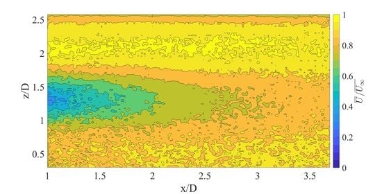
The contours of normalized $\overline{U}$ in Figure 10 and Figure 11 help fill in some of the results from power measurements. Along the centerline (Figure 10), the treatment results in lower velocity in the rotor-swept area and higher velocities below it, with the two nearly netting to zero. That there is a small region of zero difference in the middle suggests that the treatment’s effects are short-lived and perhaps only relevant in the near wake and induction zones. Similarly, along the centerline, the flow has recovered to 80-90% of the freestream by the time it reaches the end of the FOV, which is likely an indication of the research facility’s relatively high turbulence level’s acceleration of the wake decay. Together, these suggest the possibility that the wakes are recovering quickly without the treatment therefore minimizing its impact.

Recalling that the rotor tip PIV planes were taken along the centerline turbines’ rotor tips on the side nearest to turbine five, the PIV can only help to explain the fluid dynamics behind the changes in performance of turbines four and five but not three. In Figure 11, we see that the treatment has substantially decreased velocities along the rotor tip plane between rows one and two. Typically, wake velocities are highest at the rotor tips, so this may indicate increased stirring with the ambient flow during the treatment. Between rows two and three, though, the net effect is nearly zero in the rotor swept area. Both locations show some increase in velocities near the bed due to the treatment just as was observed in the centerline planes.

Interpretations of MKE can be coupled with turbine power production. In general and assuming a similar inflow, if a turbine’s power production increases, the expectation is that it will have less MKE in its wake because it extracted it in producing greater power. This does not, however, preclude the possibility of entrainment of MKE into the wake, which is a necessary part of wake dissipation, so results may not always be straightforward.

As Figure 13 and Figure 14 demonstrated, the magnitude of MKE is mostly related to the streamwise mean velocity component, and so Figure 15 maps very closely to the differences in Figure 10 and Figure 11. Looking at the centerline in Figure 14, the increase in MKE in the wake of turbine one seems opposed to the fact that its power increased during the treatment. The only other explanation for this is that the excess MKE was entrained into the wake of turbine one during the treatment, but what caused this? When a turbine’s rotation rate is increased, the pitch or distance between its tip vortices is reduced [41]. When these vortices are closer, they interact more and destabilize sooner, which accelerates the decay of the wake, allowing for net entrainment of energy in to the wake [42,43,44]. Furthermore, as seen in Figure 18, the TSR of turbine one (in fact, all the turbines) is very unsteady, which is further evidence of the rotor–generator system’s lack of inertia and the relatively higher forces in water than air. This oscillation in rotation rate may contribute to the destabilization of the tip vortices, and its effects are amplified by the increased rotation rate in accelerating wake decay [28,41].

The fact that the increase in MKE between rows two and three is quite small corresponds to the fact that turbine two produced nearly the same power in the treatment as in the control. Though turbine two had access to additional energy during the treatment, it is clear that it did not use it because we know that it was operating at its peak power point in both the treatment and the control. So where did the excess energy in the wake of turbine one go?

As shown by ref. [9], any excess energy in the wake of a turbine is concentrated around the boundary of the wake. Considering this, we would not expect to find the excess energy entrained into the centerline of the wake of turbine one during the treatment along the centerline of the wake of turbine two. Rather, we should see an increase in MKE in the rotor tip plane, which is indeed what is seen in Figure 14 between rows two and three. The rotor tip plane between rows one and two stands apart in that MKE decreased during the treatment. If it is correct that the increase in MKE along the centerline between rows one and two was due to entrainment, then an increase along the centerline would be the result of a gradient in energy from the exterior of the wake to the interior. Indeed, the results indicate more MKE in the rotor tip plane and less in the centerline during both the control and treatment. The difference may be that the increased rotation rate of turbine one during the treatment provided a more efficient mechanism for transporting energy along this gradient, thereby leading to an increase in MKE along the centerline and a decrease along the rotor tip.

The TKE is more difficult to interpret, even with the power data, because TKE can be created by a turbine’s interactions with the flow or merely advected from upstream. TKE is four to five times higher in the array than the freestream, so there is clearly an increase due to the turbines. One would expect higher turbulence levels along the centerline where the effects of the turbines are concentrated, yet TKE levels are similar in all planes and whether or not the axisymmetric assumption is made in calculating it. It is possible that the lack of phase-averaging has caused all unsteadiness in the flow, including the quasi-periodic tip vortices, to appear as turbulence, and so turbulence levels appear similar inside and at the edges of the wakes.

Putting this all together, the result of the treatment suggests the following: Turbine one was not, in fact, derated, but, due to its increase in rotation rate, its wake decayed faster and entrained energy from the ambient flow into its center. This created excess energy along the centerline of the wake and reduced energy along the edges. Turbine two was operating at peak power and so did not harvest the excess energy available to it. This energy, having passed through turbine two, was redistributed to the edges of its wake and created an increase in energy in the rotor tip plane downstream of turbine two. Turbines four and five benefited from the excess energy in the wake of turbine one and increased power, while turbine three suffered from the wakes of turbines one and two being deflected toward it.

However, an alternative explanation is also possible and should not be overlooked. As the definition of AIC requires that upstream turbines are derated, one may interpret this experiment in the opposite fashion with what has heretofore been referred to as the control actually being the implementation of AIC, while what was previously called the treatment was, in fact, the control because that is when turbine one was optimized for individual maximum power. In this view, derating turbine one by reducing its rotation rate led to slower wake decay with reduced energy along the centerline and excess energy along the edges as predicted by ref. [9]. Again, turbine two was operating at peak power in both control and treatment. Because of the reduced energy along the centerline, turbines four and five also produced less power. Turbine three produced more power because the excess energy at the edges of turbine one’s wake was deflected toward it due to bed shear. In this light, the results describe the success of conventional operation and demonstrate that AIC did not increase the total power of the array.

Looking again at Figure 14, we see that what was previously called the treatment and is currently considered the control results in less TKE everywhere except along the centerline between rows one and two, which increased. The increase in TKE there supports the theory of accelerated wake dissipation as that increase would aid in stirring out the wake and entraining the excess MKE that was also found there. The decrease in TKE everywhere else supports previous research indicating that AIC reduces loads on the turbines as turbulence levels are strongly correlated with the loading [45,46,47]. While it is not the complete picture, the sum of the centerline and rotor tip TKE in each downstream location is nearly equal in both cases. This suggests a redistribution of TKE as opposed to a difference in total.

Finally, the unequal divergences make it difficult to make comparisons between control and treatment as the data is confined to two dimensions. Indeed, it is possible that the difference in control and treatment leads to the differences in divergence. This, however, indicates that there are possibly other differences for which we cannot account without the full three-dimensional velocity field. As such, these results must be considered as suggestive of certain conclusions but not conclusive in and of themselves.

There are limitations to this study. First, as AIC is ultimately aimed at use in large wind farms, studies such as these would be better undertaken in larger (longer and wider) arrays such that the cumulative effects of wakes can be measured. While the control and treatment approach can aid in isolating desired effects, more systematic studies of the various effects of inaccurate scaling are still necessary to more rigorously confirm them as negligible bias errors in the control and treatment context. Additionally, implementing AIC with turbines whose power curves are discrete and possibly contain multiple maxima can lead to imprecise optimizations. Wake dissipation was accelerated by the high ambient turbulence levels, which made the effects of the treatment difficult to capture but was itself a consequence of ensuring Reynolds similarity of the bulk flow. We suspect the turbulence levels are also responsible for significant wear on the turbines. Indeed, this study began with 18 model turbines and was reduced to 5 by the end. As demonstrated in Figure 18, rapid fluctuations in velocity caused by the high turbulence levels led to rapid fluctuations in rotation rate. It appears that the DC motors and/or the gearboxes we used for the turbines do not handle this well, which is something the wind turbine industry would also understand.

This last point may also suggest that the induction control was not static, per se and was instead dynamic. We can say that our experiments were steady in the mean as convergence tests assured that the uncertainty in power, which tracks with rotation rate and torque, converged to within 1%. While the rapid fluctuations in rotation rate are almost certainly greater and more rapid than those that a full-scale turbine would experience while using a controller, full-scale turbines also fluctuate in response to the time-varying wind and are not actually static in their operation. Finally, all studies of dynamic induction control, of which the authors are aware in the literature, use a periodic change in controls as opposed to the random changes associated with turbulence. For these reasons, we believe that this study is still representative of static AIC, though the control, as we have referred to it, is more representative of AIC than the treatment.

Finally, the accelerated wake dissipation caused by the ambient turbulence also required turbine spacing that is less common at full-scale and potentially allowed for more interactions between wakes and turbines than is typical. This, however, is again mitigated by the control and treatment approach and the general goal to represent a fundamental fluid dynamic condition rather than an accurately scaled one.

5. Conclusions

A control and treatment investigation of axial induction control was performed using an array of five model-scale wind turbines in a wide open channel flume. Power and flow measurements were made in an attempt to connect the two and better understand the fluid dynamic impacts of AIC. Adhering to the requirement that an implementation of AIC would derate upstream turbines, and thus the final definition offered in which the original control was the AIC treatment, then the total power of the array was significantly decreased when AIC was used. The individual turbine power measurements and the flow measurements include results that support hypotheses about AIC’s effects on energy distribution in the turbines’ wakes and how it affects individual turbine power output.

Power measurements indicate that four of the five turbines decreased or maintained power production during AIC. Comparing power and flow measurements, specifically MKE, suggests that excess energy upstream was redistributed to the edges of the wake as hypothesized by ref. [9]. The changes in TKE are more difficult to interpret and require further study but support the theory that AIC reduces loads. In all, this study suggests that total array power decreases under AIC because downstream turbines suffer from decreases in MKE in the wakes of upstream turbines that have been derated and that excess MKE is found along the edges of the wake as opposed to the interior.