Demand Response Impact Evaluation: A Review of Methods for Estimating the Customer Baseline Load

Abstract

Climate neutrality is one of the greatest challenges of our century, and a decarbonised energy system is a key step towards this goal. To this end, the electricity system is expected to become more interconnected, digitalised, and flexible by engaging consumers both through microgeneration and through demand side flexibility. A successful use of these flexibility tools depends widely on the evaluation of their effects, hence the definition of methods to assess and evaluate them is essential for their implementation. In order to enable a reliable assessment of the benefits from participating in demand response, it is necessary to define a reference value (“baseline”) to allow for a fair comparison. Different methodologies have been investigated, developed, and adopted for estimating the customer baseline load. The article presents a structured overview of methods for the estimating the customer baseline load, based on a review of academic literature, existing standardisation efforts, and lessons from use cases. In particular, the article describes and focuses on the different baseline methods applied in some European H2020 projects, showing the results achieved in terms of measurement accuracy and costs in real test cases. The most suitable methodology choice among the several available depends on many factors. Some of them can be the function of the Demand Response (DR) service in the system, the broader regulatory framework for DR participation in wholesale markets, or the DR providers characteristics, and this list is not exclusive. The evaluation shows that the baseline methodology choice presents a trade-off among complexity, accuracy, and cost.

1. Introduction

As the Paris Agreement calls for climate neutrality in order to succeed in limiting global warming, the energy sector needs to continue and accelerate on its path towards decarbonisation [1]. Renewable energy sources (RES) have established themselves as the alternative solution to fossil fuels, and their share in the global energy output has increased markedly. Electricity generated globally by wind and solar energy alone has gone from 54 TWh in the year 2000 to 1871 TWh in the year 2018 [2]. However, the high penetration of RES in the electricity sector comes with new challenges for the system due to the fluctuations associated with the intermittent nature of RES.

However, the creation of liberalised electricity markets and smart electricity systems assign a significant role to final users, who are encouraged to become more active than before [3]. Microgeneration with RES, as well as energy consumption and load management on the consumers’ side, lead to more engaged participants in the grid. New technologies, such as smart meters and feedback mechanisms, are opening a series of possibilities for the users [4,5].

To decarbonise the electric grid, significant changes are needed. The objectives are to integrate the expected growing share of RES in the electricity generation, to accommodate more active users, and, at the same time, to continue providing a reliable supply through a resilient network [6].

Traditional methods to address these changes involve capital investments in the transmission and distribution system. However, making adjustments on the demand side alleviates the pressure on the grid, which can lead to investment deferral and lower costs.

The adjustments in electricity demand are carried out through the framework of Demand Response (DR), or Demand Side Flexibility (DSF). DR refers to programs aiming at reducing the overall demand peaks and congestion in the network [7]. DR programs aim to provide incentives to customers, whether industrial, commercial, or residential, to alter their consumption patterns in ways that alleviate the pressure on the grid. A dedicated tariff structure or DR program is designed for incentivising electric consumption pattern changes by end-users in response to changes in electricity price over time. Alternatively, DR can induce lower electricity demand when grid reliability is jeopardised or when some markets face high prices [8].

DR is a relevant topic, and several reviews have tackled the subject. For example, in [9], DR is discussed in the industrial and commercial sectors, along with barriers and challenges. DR models are presented for such sectors along with barriers and challenges. In [10], a review is presented on DR programs with a focus on pricing methods and optimisation algorithms. The control mechanisms of DR, the motivations to decrease power consumption, and the optimisation models for DR strategies control are presented.

The authors in [11] present a review of DR programs. The work examines factors influencing the programs (e.g., type of market, reliability, power flexibility, participants’ economic motivation, etc.), benefits, and barriers, and suggests a classification of the cases. The research examines enabling technologies and practical strategies. A relevant work on 5G IoT technologies applied on DR programs on smart grids is [12]. Its focus ranges from sensing, communication, and computing areas to smart grid security and reliability.

Ref. [13] presents a review concerning blockchain technologies applied on smart grid applications, including DR programs.

In the European Union (EU), the role of DR has been recognised and formalised. The Energy Roadmap to 2050 acknowledges the need for the distribution grid to become smarter and increase DR to accommodate distributed RES in the system [14]. The 2012 Energy Efficiency Directive (EED) 2012/27/EU, in Article 15, regulated technical and contractual actions to support DR and included provisions to enable its participation in the wholesale and balancing markets [15]. Further, Electricity Directive 2019/994/EU amended EED Article 15 and, in Article 17, specifically addressed the removal of barriers to DR aggregation [16].

The benefits of DR programs are proven to reduce electricity prices, improve system stability, and reduce price volatility [17]. The characteristics of DR to provide a cost-effective flexibility resource [18], release its market potential, and ameliorate system emergencies [19] has increased the interest in the topic.

Users participating in these programs get rebates for electricity consumption reduction during DR events. That means that a successful business case for DR depends on a convincing calculation of the BL and, consequently, of the benefits that participation in the program provides. We can describe the user’s baseline (BL) as the estimation of the electricity that would have been consumed in the absence of a DR event. To determine the demand variation value, the counterfactual BL is compared to the actual metered electricity consumption during the event [20]. BL calculation can be performed in real-time or after the event.

For the real-time calculations, a load forecasting method is applied. This requires available historic data to be used as input and a fast, reliable computation technique to process it for short-term predictions [21]. In contrast, when historical data are unavailable, the calculation is done after the event. The BL is used to verify the performance of the demand resource and to settle the compensation amount due to its provider [22]. The power, energy, and financial flows need to be redesigned based on estimated data. Methods for estimating BL should have a solid scientific basis, and the techniques or algorithms used for the estimation should deliver reliable and accurate results. Today, the high-precision techniques enabled by the availability of high computing power makes the rolling optimisation of load forecasting possible (e.g., deep learning [23], feature engineering [24]). A reliable BL is key for creating a DR offer in the market, and, without it, it would be impossible to verify effective load reduction and performance of the demand resource to settle a fair compensation [25]. Figure 1 is a visual example of the application of a BL.

There is a documented economic drawback caused by failures in the methods of BL calculation due to the lack of accuracy to predict customers’ load profiles—both for residential customers [26,27] and for commercial and industrial facilities [28]. The accuracy and reliability in the computation of the BL are recognised as a gap or a barrier to the successful roll-out of DR [10,29] and, because there is no unified method in addressing BL estimation, there is a call for an overview of best practices [30].

Although there are several reviews in the DR field, there is little with respect to baseline definition. In [31], the challenges and opportunities of load profiling techniques for DR are discussed. Focus is given, however, on reviewing the data mining techniques with respect to technical approaches, such as direct clustering, clustering evaluation criteria, and customer segmentation. The review examines data mining techniques for load profiling. To the best of our knowledge, there is no review concerning the methodologies used for calculating the baseline in today’s context where new computing capabilities meet the necessity for higher accuracy, and this is the gap that we try to cover in this article and the key incremental contribution.

This work presents and analyses the methodologies for calculating the BL. We take into consideration standardisation efforts, business initiatives, and reports, as well as novel methodologies proposed by articles in the rich literature review. Our study reviews past research and presents an updated overview and an analysis of existing methodologies for BL. Best practices for BL calculation are identified, their methods are analysed, and standardisation efforts are summarised. Additionally, this article presents how baselining is performed in practical cases, based on real DR use cases. We identified as a literature gap the collection and analysis of real tests and real application of baseline methodologies in practice, and, therefore, we reviewed the results of European funded projects for evaluation of DR. Thus, the present research has a strong focus on European H2020 projects. The insight deriving from these examples can guide both policymakers and the scientific community to address future investigations on this topic.

The text is organised as follows: Section 2 gives an insight on DR fundamentals and describes DR service providers and flexibility services. Section 3 lists the methods used to build this review; in other words, it describes the sources that have been considered for review and the goals of this reviewing procedure. Section 4 reviews the state of the art in baselining methodologies, including novel proposed methods and standardisation work. Section 5 analyses some EU smart grid projects employing DR and shows the solutions chosen for the BL definition in real cases. A discussion of the findings is presented in Section 6, whereas Section 7 concludes the article, makes recommendations and foresee limitations of this work and further research. In Appendix A, the interested reader can find expanded tables regarding the findings.

2. DR Service Providers and Flexibility Services

DR is a mechanism through which the end-user load profile can be controlled, typically with price signals or by an automated control. The end-users thus offer their flexible electricity demand as a resource to the system, which is comparable to electricity generation. Therefore, he can participate on par with electricity supply in the wholesale, balancing, and ancillary services markets.

In the conventional market model (retailer business model or retail DR), the DR is procured and under the control of utilities (e.g., distribution utilities, municipality-owned utilities) [32]. Users can aggregate and pool together their demand-side flexibility either under the control of the retailer, or, in other market models, through an independent aggregator. Local electricity markets are other models where DR can be valorised. In the context of an increasing decentralisation of the electric grid, the connection of decentralised units (e.g., microgrids) to the wholesale electricity markets is supported by the emergence of local electricity markets that incentivise the management of resources at lower levels [33]. Current research identifies that flexibility markets and local electricity markets can function either separately alongside each other or in a hybrid form [34].

DR can be implemented in two modalities. First, the implicit (price-based) DR relies on consumers reacting to time-varying electricity prices reflecting the value and cost of electricity in different time periods. The second is the explicit (incentive-driven) DR, where consumers receive a reward to change their consumption upon request. Explicit DR can be offered either directly by end-users themselves or by permitting a third party, such as an aggregator, to collect a portfolio of participants and represent them while benefiting from scale and managing capabilities inherent to their business [35,36]. Implicit DR has the advantage of being comparatively easier to implement but cannot participate in as many markets, whereas explicit DR creates controllable loads that can assist with the local RES and provides ancillary services to the distribution system [37].

Participation in DR can have both financial and non-financial motivations (e.g., environmental considerations), which can be equally influential but need to be sustained by support strategies in program implementation [38]. From the consumer point of view, in order to support them to navigate the options in DR (mainly explicit DR), it is useful to profile load mix and personal preferences, then to identify different contracts to engage different categories [39]. Consumers should be guaranteed access to reliable information to limit their confusion of choice [40]. At the consumer level, there are perceived difficulties of adoption associated with DR due to inertia, unclear policy framework, and investment costs [41]. That highlights the need for more work to increase its acceptance [42]. Among the commercial and institutional (C&I) electricity consumers, the concerns relate to interference with core processes and product quality [43], which can be addressed with adequate incentives and clear, simple, and flexible conditions of usage [44].

2.1. DSO’s and TSO’s Needs

Flexibility services should consider both distribution system operators (DSOs) and transmission system operators (TSOs) needs. Important characteristics are time frames (from real-time operation to long-term planning), identification and description of the need (type of event and possible solutions), etc. Moreover, every service that can meet SO’s needs has different characteristics: schedule, advanced notice, frequency, response time, and duration. From [45,46], we show a brief description of needs and flexibility services definition for DSO (

Table 1. DSO needs and services overview.

DSO Needs	Service Provision	Description of the Service
Power quality and loss reduction	Phase balancing	Service to maintain the balance of loads among phases to reduce losses, increase the distribution network capacity, reduce the risk of failures, and improve voltage profiles.
Extreme events’ support	- Islanding - Blackstart - Emergency load - Backup generation capacity	Services designed to increase the resiliency of distribution networks for a quick recovery from extreme events (driven mainly by natural disasters and extreme weather, whose frequency and severity might increase as a direct impact of climate change).
Network investments’ deferring (1 to 3 year timeframe)	- Voltage control (power based) - Congestion management (capacity based)	Services that aim at using flexibility in the network planning context, to solve either current or forecasted physical congestions related to reduced network capacity (overload or voltage violation).
Physical congestion control	Congestion Management: - Corrective (near real-time) - Predictive (intraday/day ahead) - Planning (months ahead)	Service required whenever insufficient power is provided to consumers due to physical limitations of the network, which can be caused by excessive power demand hours (e.g., concentrated EVs charge, power generation, etc.).
Voltage violations control	Voltage Control: - Corrective (real-time) - Predictive (intraday/day ahead) - Planning (months ahead)	Required to maintain voltages within specific standard limits and restore their values to the nominal value after grid disturbances occur. It is used to minimise reactive power flows, investments, and technical losses.

) and TSO (

Table 2. Flexibility services for TSO power system operation and planning.

Needs	Services	Types
Balancing requirements	Frequency response services	Frequency containment reserves (FCR)
		Automatic frequency restoration reserve (aFRR)
		Manual frequency restoration reserve (mFRR)
		Replacement reserves (RR)
		Fast frequency reserves (FFR)/synthetic inertia
	Innovative frequency response/quality services	Ramp control
		Smoothed production
		BRP portfolio balancing
		Damping of power system oscillations
		Local grid balancing
Congestion management	Intra-regional	Operational/Real-time
		Short-term planning
		Long-term planning
	Cross-border	Re-dispatch
		Countertrading
Non-frequency ancillary services for voltage control and restoration	Reactive power and voltage control	Obligatory reactive power service (ORPS)
		Enhanced reactive power service (ERPS)
		Fault-ride through (FRT) capability
	System restoration	Black start
		Islanding operation
Adequacy requirement	Capacity remuneration mechanisms	Strategic reserve

).

In the following paragraphs, we present analytically several BL methods, as identified in the literature review.

2.2. The Role of Aggregators

Our paper does not focus on aggregation issues, such as the complexity of aggregated baselines or the non-equal incentive problem (e.g., the incentive calculated for a group is not equal to the sum of incentives for single users [47]). For completeness, we present some basic information about load aggregation.

Aggregation can be described as a function performed by an entity to combine multiple user loads or generated electricity (i.e., for sale, purchase, or auction in an electricity market) [16].

Insight regarding the aggregators role on DR has been given in [48]. The report describes how aggregation can enable the DR participation by smaller users.

Users have to face different issues, which can be listed as:

• Lack of knowledge (both on their own consumption and electricity markets),
• Behaviour influence and engagement,
• Closed markets to small consumers,
• Risks for DR providers (failures are challenging to mitigate).

For these reasons, suppliers and independent aggregators can greatly contribute to DR development. In particular, there are several examples of markets where independent aggregators are regulated and represent the vast majority of DR participants [49,50]. This form of aggregation is described in [48] to help consumers:

• Offering a fair compensation focusing on electricity consumption services (most suppliers would not engage in services affecting their core business),
• Competing for providing customised services, based on consumer-specific load and necessities,
• Providing an IT specialised service.

However, independent aggregation is required to undergo national regulation on the law and sub-law level. Given, in many cases, the administration of electricity as a public or semi-public good, with infrastructure that needs to interoperate optimally, a more robust normative framework is required. Aggregation issues are planned to be addressed in future work, thus no further analysis is made in this paper, also because this would exponentially expand the volume of this work. For topics cited in this paragraph, the reader can refer to the future work section.

3. Methods

In this section, we present our review method and the sources of information considered.

DR is an evolving topic, as well as BL for DR subjects. We investigated the network of existing literature, its connections, and findings. Because of the vast number of interconnections and interdependences among algorithms, methods, and comparative papers, we decided to proceed with a methodological literature review to provide future direction. The objective of our contribution is to identify and review the methodologies proposed and used in practice for BL calculation. We have evaluated:

• Reports from industry associations and consulting firms involved in the research of BL definition in the field of DR;
• Scientific publications describing novel methodologies for calculating the baseline;
• Standardisation efforts focusing on methodologies for BL calculation;
• Research projects describing the methodologies used in practice for BL calculation.

The objectives were to understand the background of DR status [51], their challenges [52], and opportunities [53]. With respect to what has been used in practice, we have taken into consideration research projects realised in recent years. As of 2017, in Europe, a total of 346 projects investigating DR had been carried out or initiated [54]. Reports and publications from these sources have been consulted and have led to the identification of the research gap with respect to the BL calculation [8]. The H2020 projects have been identified using the Smart Grid Projects Outlook, focusing on projects starting after 2014, of which 23 address BL categorisation [54].

In strictly addressing the baselining methodologies for DR programs, which are technical in nature, this study reviews efforts that are not limited to the EU alone. A chronologic approach reveals that the earliest efforts have examined the implementation of DR and signalled the need for a reliable BL in the US (California) since 2002 [55]. Standardisation efforts and further studies have been regularly reported in the USA by public authorities and laboratories after that [29,56,57,58,59,60,61,62]. Case studies from the EU and other countries have been reviewed as they were reported throughout scientific publications in international journals of Science Direct and IEEE Xplore.

The review effort was carried out to identify the following:

• The type of the algorithm (mathematical model);
• How the choice of algorithm is connected with the particularities of the case study;
• The requirements to enable its implementation;
• The advantages of the chosen method;
• The disadvantages or limitations.

In what follows, we analytically present the findings of the aforementioned review work. Section 4 analytically presents the methodologies for BL calculation as these are proposed and described by industry associations and consulting firms’ initiatives (Section 4.1), by standardisation efforts (Section 4.2), by scientific papers with novel approaches (Section 4.3). In contrast, BL calculation methods used in practice are considered in Section 5, where the methods used by research projects are listed.

Results have been summarised in tables for a comparative overview. It is important to note a difference in scope between studies and reports from regulators and utility companies on one hand, and scientific projects and papers on the other hand. The point of view of regulation and the adjustments on the side of utility companies are compelled to address and accommodate DR from all customers, regardless of their size—whereas academic research offers stronger insight into residential end-user behaviour. This work compiles all findings in a non-discriminatory fashion.

4. Overview of BL Calculation Methodologies

The baseline calculation methodology is of vital importance, as it first defines all the success of DR programs. Such success depends on a credible operational procedure for determining the magnitude of load reductions, which is reflected in fair compensation for the participants. Therefore, the reliability of BL calculation methods and corresponding load variations are essential. The lack of standards and measurement procedures could lead to scepticism, dissatisfaction, and consequent disengagement of participating customers [63].

In a nutshell, it can be said that BL calculation methods involve two main steps [64]:

• A rough BL profile. The calculation is based on the decision whether to apply a day-matching method (average consumption of the same user for similar days in the past) or a regression analysis (a consumption level predicted from more data points). Other novel unstandardised methods based on artificial intelligence (AI) are in an experimental stage. This step includes data selection.
• An adjustment method to refine the rough first estimation. It is especially needed for consumption profiles that are weather sensitive.

The calculation is carried out with a computational tool. Given the field of application and its characteristics, the choice of the algorithm for the computation impacts the outcome by being more or less accurate.

The number of options available for each step leads to a large number of combinations in the process, thus the need for an overview and recommendations for a way forward.

In the following, we present the methodologies for BL calculation as found in our profound literature review, as explained in Section 3.

4.1. Estimation Methods and Practices Focused on Industry Associations and Consulting Firms Initiatives

In this paragraph, we present the methods for estimating the baseline based on initiatives from industry associations, consulting firms, or commissions. Figure 2 shows a timeline of the initiatives selected. We also present the methods developed, which have been driven by market incentives.

Back in the early 2000s, the US electricity crisis increased the interest in programs to encourage customers to reduce their peak loads [65]. In the following subsections, we present the methodologies by each business or industry association initiative.

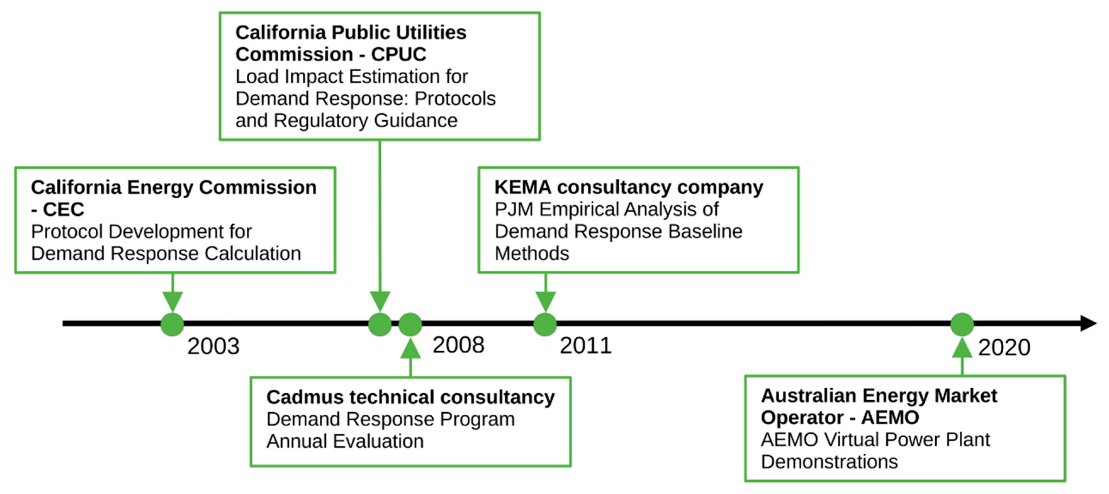
4.1.1. California Energy Commission—CEC (2003)

An early analysis of BL methods was carried out for a standardised measurement and verification (M&V) by CEC as an attempt to systematically explore BL components and their accuracy [55]. The scope of the study included small- and medium-sized customers intending to compensate users for reducing their loads on short notice (2 to 24 h). The report reviews and compares proposed methods for BL estimation based on interval-metering and identifies three components to each BL method, as summarised in

Table 3. Main components of calculation methods used in [55].

Component	Description	Examples
Data selection criteria	Criteria to determine days/period of data	- last X to Y uncurtailed business days - subset of the last business days with the highest load - full season of data - excluding and replacing days procedure
Estimation method	Calculation procedure to determine provisional BL load	- average - weather-based regression
Adjustment method	Shift or scale due to known conditions	- unadjusted - additive - scalar - weather-based

; in the table, for each component detected, we give a description and factual examples.

The BL methods were tested under various conditions to examine their accuracy. They were evaluated for:

• The simplicity of calculation,
• Minimising the burden on participants and operators (e.g., costs, ease of understanding, and ease of operation),
• Limiting the potential for gaming, ability to know the BL immediately after a curtailment or before making a curtailment decision,
• Minimising method bias (systematic tendency to over- or under-state),
• Minimising method variability; significant concerns are related to providing accurate BLs for weather-sensitive accounts, avoiding windfall credits for cool weather, or planned shut-downs.

The final recommendation is that the method for BL calculation should provide alternatives based on customer load types and operating practices. Other specific findings are listed in

Table 4. Load specific recommendation from [55].

Topic	Specific Recommendation
Default BL	The best and more practical BL is simple average of last 10 days, with an additive adjustment (two hours prior to event)
Weather-sensitive loads	Temperature-Humidity Index (THI) based adjustment is the most effective, as suggested also by PJM
Weather Regression (WR) vs. Simple Average (SA)	WR is effective, but increases data requirements; SA with adjustment results are comparable to WR ones
Highly variable loads	High variable loads are challenging despite the BL methodology chosen

.

4.1.2. California Public Utilities Commission—CPUC (2008)

Standardisation efforts for measurement and evaluation mechanisms in the DR scenarios were identified as part of the “Load Impact Estimation for Demand Response: Protocols and Regulatory Guidance”, published by CPUC [66]. To ensure verifiable energy savings, CPUC established a set of protocols, delineating a list of the minimum requirements for estimation of load impacts of DR resources, and defined a set of methodologies to determine their cost-effectiveness. The standard baselining method is highlighted as being the so-called “3-in-10”, which is “based on the hourly average of the three (3) highest energy usages on the immediate past ten (10) similar days” [56]. Further, arguably more accurate BL methods considered by CPUC follow the same principle, but for 5-in-10, or a 10-day-average BL. However, evidence suggests that the 3-day BL estimation method would lead to overestimation (and thus overpayment) in the demand bidding program, and the 10-day average method is proposed for a more reliable standard instead [58]. The study [67] evaluates the “best performing 4-in-5 day” BL method. It shows that the method is biased, with special reference to spillover (a phenomenon that occurs when customers perform energy load reductions outside the DR program’s hours).

A standard BL profile (BLP) is then improved with a so-called “Morning-of” adjustment [56]. (In some work, the nomenclature CBL—customer baseline—is used instead of BLP for the same concept. In this work, we refer to it as BLP.) For this adjustment, various methods are proposed. The two main categories are: (i) “averaging methods, which use a linear combination of hourly load values from previous days to predict the load on the event day”, and (ii) “explicit weather models, which use a formula based on local hourly temperature to predict the load” [57]. An investigation carried out in 33 C&I buildings revealed that the use of a morning-of adjustment factor for weather-sensitive C&I buildings reduces the bias and improves the accuracy of all BLP models examined. Concerning the evaluation of loads for building with low load variability, all BLP models perform reasonably well in accuracy. In contrast, for customer accounts with highly variable loads, no BLP model produced satisfactory results [57].

As for industrial consumers, it can be challenging for companies to follow a BL development approach that is unsuitable for the organisation’s size, production profile, culture, or geography. In order to evaluate a customised BLP for a facility, the complexity and priorities of the site need to be included in the calculation, with parameters such as business cycle variability, numbers of product lines, and weather-related impact on energy performance [59].

The purpose and use of the BLP are exemplified with an evaluation of the impact of DR. The impact evaluation can, in turn, be carried out through one of three broad categories—day-matching, regression analysis, and other—each with different requirements, as summarised in

Table 5. DR impact estimation methods and their application [66].

Method	Description	Comments
Day-matching	- Difference between a reference value and the actual load on an event day - Relevant days are selected	- Useful for ex post impact estimation - Can use weather adjustments - Primary approach for large C&I customers - Difficulties estimating uncertainty adjusted impact estimates
Regression analysis	- Relies on statistical analysis to develop a mathematical model that considers a range of influencing factors (e.g., weather variables, participant characteristics, etc.) - Preferred whenever ex ante estimation is also required	- Robust and flexible - Requires more skills and it is less transparent - Permits one to quantify the influence of specific characteristics (e.g., heat build-up, multi-day events, etc.) - Should be considered as the default option for the majority of applications
Other methods	Include sub-metering, engineering analysis, duty-cycle analysis, and experimentation	- Specific conditions (e.g., erratic consumer behaviour, lack of variability, data limitations, budget constraints, etc.) - Engineering analysis are when there is no behavioural influence by the consumers, operational experimentation, and measurement or verification activities - Possible combination with regression analysis

:

4.1.3. Cadmus Technical Consulting Group (2008)

An evaluation of predictive accuracy of BL calculation in 92 facilities of C&I, government, non-profit, and education (GNE) customers found that regression methods are the most accurate for 87% of the cases. Upon a closer look, for all the small C&I and GNE users, it is confirmed to be the right choice, but accuracy in the case of large C&I users is sufficient only 48% of the time. Regression does not predict well for facilities with highly variable day-to-day consumption in the hours of the event. There, the best predictor of consumption is consumption in recent previous days, therefore many large C&I facilities selected X-of-Y-previous-day baselining methods [60].

4.1.4. KEMA Consultancy Company (2011)

In 2011, KEMA prepared for PJM an analysis for DR options and their adjustments [68]. The aim was to evaluate accuracy, bias, and feasibility, and attempt to associate a user load with a specific BL method. The analysis is based on data requested from PJM distribution companies, both program participants and control groups. The duration was over a 28-month period. Adjustment tested have been additive, multiplicative, and PJM weather sensitive. The BL methods considered included several average, matching, and regression methods.

4.1.5. Australian Energy Market Operator—AEMO (2020)

In 2020, AEMO prepared a report to provide an update to the Australian Renewable Energy Agency (ARENA) and the industry [69]. The document gives insight into a virtual power plant (VPP). It describes findings regarding DER load generation forecasting and network support services, such as frequency control ancillary services (FCAS). Regarding FCAS, it calculates a BL using power measurement for the last 5 s before frequency excursions. Results suggest an interesting capability of VPP to provide FCAS and react to energy market price signals.

4.1.6. Work for Southern California Edison

Another interesting work, validated through Southern California Edison’s residential smart meter data, is [70]. There have been developed three statistical BL methods to forecast load BL. The first two are the regression spline model and mixed effect change point model, and they fall within the category of Type II BL (see Table 6 for definitions). The results are compared with the fixed effect model (a simplified version of the regression spline model) and Type I BL methodology (based on the estimation on similar day-based algorithm). The proposed forecasting models produced a more accurate forecast for BL load.

4.1.7. Programs Driven by Market Incentives and Manipulation Risks

Alternatives to statistical and computational BL estimation methods have been examined based on market incentives, and focus has been given on administrative and contractual approaches.

The weaknesses that contractual approaches aim to address have to do with the opportunities to game the system. For example, by using last year’s data for computation, consumers can be effectively incentivised to inflate their BLs so as to increase the DR program payment. Considering wholesale markets, work in [71] described how demand reduction payment can bring to customers BL inflating during normal peak periods and exaggerate demand reduction during DR events. The suggestions proposed to define the BL are (i) an aggregate BL approach, (ii) a “contractual baseline in which the marginal consumption decision is based on the time-varying wholesale rate”, and (iii) an adjustment of demand reduction compensation with wholesale rate minus the retail rate. Because the as-called “incentive for manipulation” is undermining DR programs, studies suggest policymakers consider the threat by modifying DR market rules. As options to consider, the authors suggest evaluating marginal cost pricing, as well as DR in the ancillary and reserve market [72].

In particular, during uncertain DR events’ schedules, users could artificially inflate BL, which would have a significant impact on the effectiveness of the programs [73].

Several attempts have been put in place to analyse the issue (e.g., formulating payoff-maximising user function [74]). Manipulation attempts often are difficult to detect, due to the asymmetric information available between users and market administrators [75].

The method of full locational marginal price (LMP) payment is sometimes called to be a double payment for demand reductions. The reason is that the DR provider would benefit both from the cost saving of not consuming an increment of electricity plus an LMP payment for not consuming the same amount of electricity [76,77].

This could induce excessive demand reduction, compromising the efficiency of DR programs. To correct these shortcomings, contractual obligations would have to be added to the estimated BLP [78].

The alternative approaches that bypass statistical methods are in fact addressing the weaknesses of conventional BLP estimation methods. In flexibility markets at the distribution level, BL calculation based on averaging or interpolation leads to concerns about manipulation [79] and inflating, whereas methods such as those based on regression add complexity and administrative costs, suggesting that BL are not suitable for those markets [80].

4.2. Standards

BLP estimation output complexity increases with each choice made in the estimation process. Several standardisation attempts have tried to set the guidelines for evaluating the BLs while performing DR. Similarities may be found between the approaches described by standards and the approaches in scientific articles or initiatives from industry associations and consulting firms. However, as the goal of this work is to present all findings in a non-discriminatory fashion, as stated in Section 3, it is vital to present BL calculation methods, as these are demonstrated in standards. In the following, the reader can find summarised information of standardisation attempts so far.

4.2.1. National Action Plan for Demand Response—NAPDR

In the US, following the Energy Independence and Security Act in 2007 [81], the Federal Energy Regulatory Commission (FERC) produced a report assessing the DR potential where measurement of customer BL is considered an issue [82]. The North American Energy Standards Board (NAESB) developed a Business Practice Standards for DR M&V [83]. The document defines broad types of DR programs and different performance methods. To provide guidance on M&V methods, the National Forum on the National Action Plan for Demand Response (NAPDR) produced a report aimed at helping to advance the development of DR resources. [82] Following the terminology and framework of NAESB, EnerNOC released a white paper [84] and a report [59], primarily to investigate how to measure DR resources and to establish an energy BL for industrial facilities.

NAESB standards entail five BL evaluation methods, as listed in Table 6.

Table 6. BL evaluation methods in [85].

Method	Description
Maximum Base Load	Demand resource keeps electricity usage below a certain level
Meter Before/Meter After	Electricity demand is compared during the DR time occurrence and similar readings before the DR event
BL Type I	Uses historical interval meter data of the demand resource
BL Type II	Uses statistical sampling for an aggregated demand resource to estimate electricity usage
Metering Generator Output	Considers the output of a generator, located behind the demand resource’s revenue meter, then the demand reduction value is based on this output

Table 6. BL evaluation methods in [85].

Method	Description
Maximum Base Load	Demand resource keeps electricity usage below a certain level
Meter Before/Meter After	Electricity demand is compared during the DR time occurrence and similar readings before the DR event
BL Type I	Uses historical interval meter data of the demand resource
BL Type II	Uses statistical sampling for an aggregated demand resource to estimate electricity usage
Metering Generator Output	Considers the output of a generator, located behind the demand resource’s revenue meter, then the demand reduction value is based on this output

Regarding BL characteristics for evaluation, NAESB notes: “baseline window, calculation types, sampling precision, exclusion rules, baseline adjustments, and adjustment windows”. For the BL window, the 10 most recent program eligible non-event days are calculated. Additionally, it is suggested to account for further information regarding the event (e.g., real-time telemetry, performance window, measurement type, etc.)

The methods in Table 6 have been evaluated with reference to the service provided (energy, capacity, reserves, and regulation) by [85] (IRC 2008) and [86] (PJM 2018). The findings of the studies are summarised in

Table 7. Methodologies used for BL calculation as used by IRC and PJM in [85,86].

Performance Evaluation Type	Service Type
	Energy	Capacity	Reserves	Regulation
Maximum Base Load	IRC	IRC, PJM	-	-
Meter Before/Meter After	IRC	IRC	IRC, PJM	IRC, PJM
BL Type I	IRC, PJM	IRC	IRC	-
BL Type II	IRC	IRC	IRC	-
Metering Generator Output	IRC	IRC	IRC	IRC

.

For a deeper analysis of service types per BL method, we recommend further evaluation on the topic.

4.2.2. International Performance Measurement and Verification Protocol—IPMVP

The IPMVP protocol offers a framework for carrying out and evaluating efficiency and demand management measures [87].

Regarding energy, it defines energy conservation measures (ECM) as a set of actions for energy conservation, efficiency improvement, or demand management.

The protocol points out that demand savings cannot be measured directly, because savings represent the absence of demand. For that reason, “savings are determined by comparing measured consumption or demand before and after implementation of a program”. The comparison among before and after demand follows the general M&V equation:

Savings = (Baseline Period Energy − Reporting Period Energy) ± Adjustments

The protocol aims at implementing a quality M&V process. It lists considerations about BL period selection, reporting period, and types of adjustments. BL period and reporting period are set to properly represent operating modes. Particular emphasis is placed on measurement boundaries (entire facility or a portion), intended as the choice of granularity of measurements for determining savings.

The choice of the options depends on the purpose of the reporting and relevant data available on site.

Following the [87] principles and guidelines, the EU Project DRIMPAC 2020 [88] developed an example of a regression model. In the regression model, the dependent variable is energy demand (E_D). For the independent variables (defined as H(t) humidity, T_out(t) outdoors temperature, WD_N normal weekday, WD_h holiday weekday, WE weekend days, T_stamp timestamp, O_ill(t) outdoors illumination, H_DM(t) heating degree minutes, and C_DM(t) cooling degree minutes), historical data are used (previous 24 h); e is the error of the regression model.

The multi-variate regression model is proposed in the following form:

$$E_D=a+b_1\ast H+b_2\ast T_{out}+b_3\ast W{D}_n+b_4\ast W{D}_h+b_5\ast WE+b_6\ast T_{stamp}+b_7\ast O_{ill}+b_8\ast H_{DM}+b_9\ast C_{DM}+e$$

From the model developed for energy demand, it is possible to extract the model for power demand, as these two quantities are proportional:

$$P_D\propto E_D$$

The model is applied to past values to extract the coefficients (a, b_i), then the BL is calculated. The BL shows the consumption that would have taken place without any DR event with reference to the previous day of the event. The above model is generic and can include all possible parameters. The scope of the method is to include the parameters that impact the BL calculation for each specific site.

The above is only an example for evaluating the baseline. Numerous other examples can be found in Section 4.3—Novel Tools for Estimation. In general, as time passes and DR becomes more and more popular in the scientific community, it is expected that more innovative models and more accurate estimation methods will emerge for the BL calculation.

4.2.3. Energy Management Systems—ISO 50006:2014

According to ISO 50006:2014 [30], in order to measure and quantify energy performance, there are two variables to consider: energy performance indicator (EnPI) and energy BL (EnB). EnPI is defined as “a measure or value that quantifies results related to energy efficiency, use and consumption in facility, systems, processes and equipment”. EnB, instead, refers to energy performance during a specific time period, and it is used as a reference during the implementation of actions for energy performance improvement. EnB is set to the value of EnPI during the baselining period. A comparison with EnPIs of the reporting period illustrates the improvement in energy performance. To establish an EnB, it is suggested to first establish the purpose of the calculation, then determine a suitable data period, then collect the data, and, finally, determine and test the EnB.

4.3. Novel Tools for Estimation

BL evaluation and adjustment techniques for DR are benefitting from the improved computational capabilities of recent years, which allow processing of large amounts of data and near-real-time decision-making—both important enablers of DR. Machine learning (ML) techniques, such as deep learning (DL), support vector regression (SVR), linear regression (LR), neural networks (NN), and genetic programming (GP), are now accessible for use in problems of system optimisation [89]. Their application in DR means that more data can be processed (i.e., averaged) in less time, which leads to more accurate estimates and greater flexibility.

Recent progress in the application of ML shows success in load forecasting [90,91,92,93], modelling [17], and control [94,95]. Learning-based DR management system approaches in buildings have been studied [96], considering also comfort constraints for the users [97,98]. There have been attempts using ML to classify consumers concerning potential performance [99,100] and to forecast the impact of their decisions in relation to long-term costs and schedules of residential device usage [101]. ML and, more specifically, NN have also been applied to the modelling of electricity prices as multi-agent systems [102,103], for optimisation of DSM of power system management in real-time [104], and for electrical consumption forecasting [105]. GP has shown to have good results, with low approximation error and computational cost on widely known energy efficiency forecast datasets [106].

In view of these results, application of ML techniques has been sought in the estimation of BLP for DR. In a comparative study of five ML techniques—high X of Y, last Y days, regression, neural network, and polynomial interpolation—carried out on actual smart meter data, NN and polynomial interpolation outperformed the other methodologies in terms of reliability of prediction, lowering the estimation error [107,108]. NN has also shown useful application in BL calculation for industrial facilities [109]. Regarding HVAC related loads, ref. [24] applies a feature engineering method. It uses a combination of feature selection and hyperparameter tuning applied to various ML models, with positive results. For residential users, the highest accuracy of BL calculation appears to be achieved through probabilistic methods [110,111], whereas a Bayesian inference approach has been shown to support real-time updating needs [112]. Clustering customers in order to reduce heterogeneity and improve predictability can also be carried out with ML techniques [113].

A particular point of interest is the increasing penetration of distributed photovoltaic systems (DPVS), which leads to volatile customer actual load data. Estimating DPVS output correctly has direct implications on the BLP estimation. ML techniques have proved to provide successful support, which has been explored with the SVR-based model approach [114] and k-means clustering algorithms combined with decupling-based BLP estimation for residential customers [115]. Clustering by k-means adopted alone, used to categorise consumers based on their load profile, has shown to have a good performance on the accuracy, bias, variability, and reliability in terms of prediction [116].

Concerning the residential building sector, in [117], there is a review on the developments of DR programs, with specific reference to methodologies and procedures for assessing building energy flexibility with numerical models and control algorithms. A useful taxonomy for such models can be found in [118]. One of the main findings is that heuristic approaches can provide approximations with acceptable accuracy in relatively short time frames, then a more analytical approach should be evaluated. The study in [117] shows how a combination of different approaches is useful. The techniques adopted include linear integer programming, different machine learning techniques, and model predictive control. Overall, to accurately assess its performances, the combined approach deserves further investigation.

Apart from being tools used for the methods of BL estimation and adjustment, ML techniques show potential for becoming themselves a method for BL estimation. Through unsupervised learning, a BLP of residential users could be generated, which in some studies outperformed day-matching techniques [119,120].

There are also other models proposed in the literature for calculating the baseline. An example is the model proposed in [121], which takes into account simple adjustment factors through physically based models. According to the authors, gaming responses are detected before and after DR. Such a model can be applied for some loads, but it depends on end-use share and the customer segment.

Another interesting proposal is the control group method [122,123]. It uses historical data of the non-DR customers who exhibit the most similar load patterns to the DR participants [124] and sometimes applies a clustering technique [122,125]. The method presents statistically significantly better overall performance compared to several day-matching and regression techniques. The main advantage is the possibility to use readily available historical data from other users. That is valuable, for example, in the case of a new customer. For instance, in [123] authors obtain the data of the control group, selecting from the entire group monitored only the users who are not participating in DR, for the round considered. Other methods are to include costumers not participating at all in the program, or creating a virtual control group and then using a difference-in-difference approach for comparisons. Another drawback is that the technique is challenged by DPSV systems and, in general, on-site energy production systems [122]. The method could become expensive, in terms of resources, as the precision increases. In recent years, a closed-loop mechanism coupled with adjustments, with extensive comparisons with day and regression-based, has shown to have promising results, but needs further research on probabilistic estimation [126].

In [127,128], authors described an experimental demonstration of baseline load forecasting using frequency regulation applied to commercial buildings. They modelled the facilities and used a hierarchical control with a predictive controller. The results showed how this method is appropriate for commercial facilities.

Finally, there have been comparative studies [129,130,131,132] evaluating the “self-reported baseline” method combined with a calling probability mechanism of participation to DR of the users.

5. BL Calculation Methods in Practice: H2020 Projects

European innovation projects have an important role regarding examples of practical use of different BL methods. Twenty-three projects were identified among H2020 projects, addressing BL calculation in real cases.

Table 8. H2020 projects and methods used for defining the BL.

n.	Ref.	Project	Methods and Data Used for BL
1	[133]	ADDRESS	Similar days, historical data
2	[134]	AnyPLACE	Load forecasting
3	[135]	CITYOPT	Statistical method to calculate the power saved, particularly in energy efficiency
4	[136]	CityZen Amsterdam	Historical data; 1-year monitoring
5	[137]	DELTA	Regression model based on historical data, weather parameters, type of day used for BL; standards such as ISO, NAPDR, IPMVP are listed
6	[138]	DR-BoB	IPMVP for yearly global evaluation of additional energy efficiency measures; historical data
7	[88]	DRIMPAC	Standards such as ISO, NAPDR, IPMVP are listed; regression model based on historical data, weather parameters, type of day used for BL
8	[139]	DRIVE	Historical data (measurements and smart meter data)
9	[140]	ECOGRID	Historical data; price and load forecasts
10	[141]	eDREAM	Historical data
11	[142]	EnergyLab NordHavn—New Urban Energy Infrastructure	Data collection
12	[143]	Flex4Grid	Measurements play key role; control and user groups are used for comparison
13	[144]	FlexCoop	Takes into account IPMVP and NAPDR; algorithms are created; user-centric approach is used
14	[145]	IndustRE	Historical data
15	[146]	NOBEL-GRID	Historical data
16	[147]	P2PSmarTest	Historical data used; day-matching plus regression models; window between 5–10 days
17	[148]	RESPOND	Measurements for the BL
18	[149]	Semiah	Measurements and simulations to get modified load profiles
19	[150]	SINFONIA	Energy consumption data for each building within a district simulation for all buildings within the district
20	[151]	SmarterEMC2	Measurements are used to define the BL
21	[152]	SmartUp	Measurements before and after the event
22	[153]	Upgrid	Consumption data plus HEMS simulating BL (simulation tools used)
23	[154]	Vulnerable Consumers and energy efficiency	two groups of customers: control (for the BL) plus intervention group (for DR actions)Historical data; previous similar days

provides an overview of the initiatives.

As summarised in Table 8, four projects explicitly refer to standards, such as the IPMVP, for determining the BL. Most of the projects (12 in total) use historical data to define the BL, whereas five projects (23% of our sample) note that simulations and statistical methods are used to define the BL. In general, it is of interest to note that 77% of the projects use historical data for BL. Some of these public deliverables do not include information about the accuracy and precision of their methods, so, it is not easy to extract such information. However, for many of these projects, more detailed information about the precision and accuracy of these approaches used is included in the in-depth description provided in their supporting documentation. The reader is directed to the relevant references (deliverables) of the projects in order to identify such information.

6. Summary and Discussion

This study examined literature, reports, and scientific publications addressing the calculation of the BLP, which is necessary to carry out DR programs. Three standardisation efforts were identified, providing guidelines for BL estimation. Finally, 23 European H2020 projects were analysed, with a focus on the methods applied to baselining definition. The discussion of the overview looks at the challenges and opportunities for each method. First (Section 6.1), we summarise the methodologies presented in each one of our identified sources of information. We give a clear picture of what is being presented in the literature review, thus summarising the information analysed in detail in Section 4. Next (Section 6.2), we discuss the findings by summing up all the methods for calculating the baseline found in the literature. In this way, we present all the methodologies, their level of complexity, and the case in which it is best to use one particular method, i.e., which customers group is best suitable for using a particular methodology.

6.1. Summary

Table 9. Summary of BL calculation methodologies proposed by reviewed projects.

Report/Study	Method/Guidelines for BL
Xenergy document for the analysis of baselining [55]	Interval metering, based on three components: Data selection criteria (which days and time periods of data used) Estimation method (the calculation procedure) Adjustment method (scales the provisional BL)
CPUC studies [66]	Standardised M&V mechanisms: Day-matching methods: good for ex post impact estimates preferable for use in customer settlement Regression-based methods: most common/default option; preferred method whenever ex ante estimation is also required
Report and studies by Ernest Orlando Lawrence National Lab [57,61,62]	In [57], the models are sorted into two groups: averaging methods: use of a linear combination of hourly load values from previous days to predict the load on the event day explicit weather models: use a formula based on local hourly temperature to predict the load Refs. [61,62] use linear regression method modelling: 15 min interval, whole building electric load data weather data effects
Report by Quantum Consulting for the Southern Edison Company [58]	Different methodologies for BL: For the day-ahead program, it is suggested to consider changing the 3-day DBP BL method for program settlement Customer-specific BL: sub-metering used to improve the reliability of impact estimates
DR in wholesale electricity markets: the choice of customer BL [78]	Different methodologies for BLs: Administrative customer BL, estimate the users’ consumption levels using, for example, the last year’s data contractual customer BL approach: for a robust framework that restores efficient DR under full locational marginal price (LMP) payment
Report by Northwest Energy Efficiency Alliance (NEEA) [59]	Different steps for defining the BL: Establish the boundaries of the facility Identify the energy sources Determine the BL period duration and the specific historical time frame Define energy performance indicators (EnPIs), BL adjustment is determined
KEMA report by PJM [68]	Several methods for each category: Average Matching Regression Different adjustment tested (additive, ratio, regression-based)
Evaluation on DR by CADMUS Group for PPL Electric Utilities [60]	Different BL modelling approaches: Several-day matching: when there is highly variable day-to-day consumption in the hours of the event Regression methods: for 87% of the overall facilities, the regression method is the most accurate one

shows the BL calculation methodologies proposed by the analysed reports and studies.

Table 10. Guidelines for BL calculation according to standards and protocols.

Standard/Protocol	Method/Guidelines for Baselining
NAPDR [20]	Specific parameters are defined: BL window (the 10 most recent program eligible non-event days), sampling precision and accuracy, BL window, and exclusion rules
IPMVP [87]	It considers: period selection, reporting period, and types of adjustments. Measurement boundaries are important: 1 retrofit-isolation—key parameter measurement 2 retrofit isolation—all parameter measurement 3 whole facility: the measurements performed at the facility level 4 calibrated simulation: all calculations based on simulations
ISO 50006:2014 [30]	EnPI quantifies results related to energy consumption. EnB refers to energy performance during a specific period (reference). A comparison between EnPI and EnB illustrates the improvement in energy performance. To establish an EnB it must set the purpose of the calculation and a suitable data period. Collection of data and determination and test of EnB follow.

lists the BL calculation standards. As can be seen from the tables, many of the methods described share some common points, for example, using a window of days for utilising data for creating the baseline. Regression models and day-matching models are referred to in the tables, meaning that these techniques are popular for extracting the baseline. Apart from this, there are differences for each model and, in the end, it depends on the system needs as to which model will be chosen. This report does not aim to favour one technique or another, but to list the techniques and leave it up to the system designer to choose the most suitable method. This section describes some of the characteristics of the techniques found in the literature and thus presents some kind of comparison among them.

Table 10 summarises the guidelines for BL calculation from dedicated standards and protocols.

Table 9 and Table 10 indicate that the estimation of BLP relies most often on previous metering data and highlights the relevance of period and duration selection for accurate BL calculation. Day-matching approaches and regression models are the two main categories used for BL estimation in research as well as in practice and are referenced by the standards. Adjustment of the BLP is especially important with regard to weather effects. Other novel approaches, different from day-matching and regression, and not standardised yet, rely on computational capabilities and AI.

For a comprehensive listing of the main methods and adjustments identified in this review, the reader can refer to Appendix A.

The complexity of the decision process of the method for BL calculation is posed by the availability of a large number of options at each step.

The number of parameters, the availability of data, and the choice of algorithms determine the level of accuracy in the BL calculation. As reflected in the analysis of H2020 projects, the choice of BL calculation method is not standardised, and there is no “best method”—but rather, a “most suitable method” for each case.

Regarding the day-matching techniques, the BL calculation should provide alternatives based on customer load types and operating practices [55], whereas more accurate BLs for many large C&I facilities are needed [60]. However, for regression models, we point out that they are generally more complex, harder to understand, and include a higher cost. They provide a BL corresponding to particular weather conditions of curtailment day. However, if observations do not feature extreme conditions as the curtailment day, the model estimate may be inaccurate. In case the account is not weather-sensitive, it may be less accurate than simpler methods. Models that incorporate temperature (e.g., explicit weather models) improve accuracy and avoid bias [57]. However, the model could have significant errors associated with the correlation between regression parameters and the autocorrelation of their residuals [26]. Regression models give the most accurate BLs for many C&I customers and GNE facilities [60]. Regarding novel approaches, such as polynomial regression, it is efficient when applied to industrial facilities [109].

As for other probabilistic estimation techniques, residential customers are characterised by uncertainty in consumption behaviour. The GP-based methods can actively discover customer patterns and embed such knowledge into learning in a short time, improving the accuracy of the prediction [111]. The BLR approach provides an improved forecast of hourly load where real-time model prediction is needed [112].

The adjustment of the baseline is also of crucial importance apart from defining the baseline itself, as it can be decisive for the accuracy and precision of the baseline. Thus, the adjustments that can take place for improving the rough BLP estimation belong to three main categories:

• Pre-curtailment hours adjustments,
• Weather-based adjustments, and
• Structural change-based adjustments.

All of the adjustment methods above are noted in numerous references that have been analysed in this work. The exact article where a specific adjustment method is analysed can be found in the information presented in Appendix A. It should be noted that all three methods have their pros and cons.

Specifically, the first method (pre-curtailment hours adjustment) can adjust well for alterations in the load that occur constantly during the day, and it can provide very good accuracy if the duration of the adjustment is at least 2 h before curtailment. However, if the load changes during the curtailment period, the accuracy drops. This method may be inappropriate if day-to-day load variation is constant over the day. Literature indicates that the appropriate pre-curtailment increase in load (e.g., pre-cooling) can result in overstated BL, whereas the pre-curtailment decrease in load in response to a curtailment request (e.g., long ramp-down, cancelling a shift) can result in an understated BL. Applying a morning adjustment factor significantly reduces bias and improves the accuracy of the models examined [57].

With respect to the second method (weather-based adjustments), as the name implies, it considers weather conditions for the adjustment, which can be considered as an advantage, as weather conditions can greatly influence the consumption, and thus the baseline. A disadvantage can be noted in the case when predictions of weather do not correspond to reality, and it adds complexity to the overall procedure. In addition, adjustments may not be known to the customer until after the curtailment period, which is another disadvantage. The weather-based adjustments are of particular relevance for residential customers and C&I buildings, but not in industrial process loads. Weather data may occasionally contain erroneous values, which produce outliers in the model predictions, therefore weather data should be screened for consistency [57].

Finally, the last method, namely the structural change-based adjustments, can contribute to adapting the baseline to structural changes or to address a large facility’s change of occupation. However, a disadvantage of this method can be that potential input and approval from stakeholders may be necessary. Structural change-based adjustments can be used for industrial facilities, and the organisation should define intervals at which it reviews the key characteristics of its operations that determine energy performance.

The adjustment methods can improve the accuracy and precision of the baseline definition, and thus they can contribute to a more precise DR program with accurate calculations for the load curtailed and thus lead to accurate remunerations for customers. In Appendix A, the reader can find summarised information with respect to the different adjustment methods.

6.2. Discussion

In general, we identify eight methodologies for defining the baseline:

• Day-matching (DM);
• Regression;
• Control group;
• Self-reported BL;
• Polynomial regression (PR);
• Neural networks (NN);
• Other probabilistic estimation techniques;
• Unsupervised learning techniques.

Table 11. Summary of BL methodologies and their evaluation.

Category	Complexity	Accuracy	Estimated Cost (If Smart Meters and Sensors are Already Installed)	Optimal Target Group(s)	Critical Target Group(s)
Day-matching (DM)	Low * (* if historical data are available)	Low/Medium	Low	Large C&I users	- Weather sensitive users - Prosumers (renewable production) - Variable load customers
Regression	Medium/High * (* requires appropriate evaluation of variables and data range)	Medium	Low	Weather sensitive users	Depends on the model
Control group	Low * (* if historical data are available)	Medium	Low	New users	Prosumers (renewable production and storage)
Self-reported BL	Low * (* if historical data are available to the user)	Medium	Low	n/a	n/a
Polynomial regression (PR)	High * (* difficult to determine the degree of the polynomial)	Medium * (* boundary effects)	Low	Industrial factories	n/a
Neural networks (NN)	High * (* difficult to find an architecture, requires more data than other methods)	Medium/High * (* issues with generalisation)	Low * (* trained staff could be required)	Industrial factories	n/a
Other probabilistic estimation techniques	Medium	High	Low * (* trained staff could be required)	- Residential users - Prosumers (renewable production)	n/a
Unsupervised learning (UL) techniques	Medium/High * (* difficult to find an architecture)	High	Low * (* trained staff could be required)	- Residential users - Prosumers (renewable production)	n/a

shows our findings exploring the most recent literature on BL methodologies. It summarises the methods, their level of complexity, and optimal and critical target groups identified. For each method, we present the indicative cost, along with information about the accuracy of each technique. In this way, the user can have a rough idea about the pros and cons of each method. There is a variety of methodologies to choose to define the baseline. In addition, several parameters play a role in deciding the most suitable methodology, such as the consumer group for which the baseline is calculated, the overall complexity that the system can afford, and the total cost, to name some of these parameters. We have evaluated and compared all these factors, with their utilisation in the literature. The results of the comparison give a clear picture of which can be the most suitable BL out of the available ones. We can state that there is no unique solution that fits all needs.

Table 11 aims at clarifying to the reader the basic pros and cons of these methods and sheds some light on the available methodologies that can be applied. The final decision is up to the baseline designer according to the system’s needs and the aforementioned parameters and trade-offs. It should be also noted at this point that, especially for the accuracy and complexity of each method, not all sources have clear evidence. Thus, analysing the accuracy and complexity of only some of the methods would have been unfair towards the rest. However, analysing accuracy and complexity issues may result in an even more lengthy paper, thus losing the focus of the current work, which is to present the methodologies and give a fair basic comparison. Therefore, we are limited at this point in presenting only basic information with respect to accuracy and complexity. It is planned for further work to analyse such issues for the baseline calculation methodologies. It is reminded at this point that the scope of the paper is to list the methodologies and give the reader an idea of possible methodologies among which to choose the one that would best fit the needs of the system.

Regarding the more traditional methodologies, if historical data are available, previous research shows that, for day-matching, complexity of implementation is low. For the regression methods, it is medium or high, depending on the complexity of the evaluation of the variables. However, day matching is lower in accuracy compared to regression. If smart meters are available, both have a small estimated cost. For the same reason, PR and control require a relatively low budget. It has a medium accuracy but quite high complexity, due to the difficulties of evaluating the polynomial degree. Self-reported BL shows to be interesting for DR evaluation if combined with a random method of recruitment from a pool of participants. NNs have medium to high results in accuracy, with the drawback of having a more sophisticated implementation, especially regarding their architecture. Considering the big family of other probabilistic estimation techniques, they tend to have a high accuracy in results and medium complexity. The UL techniques have also a high accuracy and the same downside of being quite complex to implement. For all the ML and probabilistic estimation techniques, the cost estimation assessment is not straightforward. It should consider, for example, the presence of trained staff for implementation.

The last two columns of Table 11 focus on the target groups suitable for each method. It is clear that large C&I users, having a more predictable load profile, can have acceptable results from profiles calculated using relatively simple BL, such as DM. The most critical groups are the weather-sensitive consumers and the prosumers, especially where renewable energy production is involved, due to the uncertainty of weather forecasts and outdoor environment variables. This is where the more innovative techniques can help, where UL and probabilistic estimation techniques prove to be more flexible and to have a wider range of applications.

In line with DR engagement in practice, large consumers can participate with large controllable loads but have strong constraints. Thus, they need a customised BL and the possibility of influencing the DR participation in real-time. The choice of BL calculation principles depends on the customisation needs, and the choice of tools to carry it out in a cost-efficient and rapid way. Small residential consumers pose different challenges and opportunities for DR engagement. The participation in the system is small by nature, but stable, therefore a more generalised BL can be used. For this segment, low-complexity BL calculation principles are appropriate, such as day matching, but it comes with a trade-off in accuracy. In this case, the cost savings achieved through a low-complexity implementation are challenged by the possible unrealised gains due to inaccurate results in BL calculation. However, residential consumers have another particularity: due to scale effects, this sector offers the possibility of novel methods development for BL calculation that are based on machine learning and require large amounts of data to achieve performance.

Table 12. Comparison of adjustment methods applied to BL.

Adjustment Method	Description	Complexity	Accuracy
Pre-curtailment hours adjustments	Additive	Low	Low/Medium
	Scalar	Low	Low/Medium
	last 2 h before curtailment period	Low	Medium
	3rd and 4th hour before curtailment period	Low	Medium
Weather-based adjustment	Any	Medium/High	Medium/High
Structural changes-based adjustments	Update of the BL based on energy source, operational, business, energy management systems changes	Low	Medium/High

identifies the adjustment methods used to improve the first estimation of the BL.

7. Conclusions

Although consumer engagement in demand response has documented benefits for the electricity system and the consumers alike, the correct measurement of the benefits is essential in order to provide a convincing business case and reward participation. For the determination of a reference value (BL), the challenge is not the calculation itself, but the identification of the most suitable method for the application considered most accurate and most cost-efficient, while also fair. Current methods rely on one of two general standardised principles, each addressed with one out of several mathematical approaches, which in turn can be carried out with one of many computational tools, pertaining to different levels of accuracy and bias, as well as costs and requirements. Thus, the outcome is heavily case-specific, and the emergence of one definitive BL calculation method is improbable.

In support of DR stakeholders from policymakers, academia, and practitioners, this work reviews existing methods for the calculation of BL load profiles of electricity consumers, knowing that they are expected to strike an adequate balance among desirable criteria, such as accuracy, simplicity, and integrity. For this reason, we review numerous articles found in the literature that propose novel methods for calculating the baseline, along with reports from business initiatives or consultancy firms, as well as standardisation efforts. We analyse the methods proposed by each literature source by summarising the methodologies proposed, listing their pros and cons with respect to complexity, cost, and customer groups issues. This way, the reader can have a clear picture of the existing methodologies together with a fair comparison of them. The aim is to provide clarity by identifying core principles, influencing factors, and appropriate algorithms to carry out the computation. The assessment of baselining in European real project applications has supported the validation of results.

In general, eight methodologies have been identified for defining the baseline: day-matching (DM); regression; control group; self-reported BL; polynomial regression (PR); neural networks (NN); other probabilistic estimation techniques; unsupervised learning techniques. Each of these methodologies has been analysed and a fair comparison of them is presented in terms of their advantages and disadvantages. We found that the choice of the best methodology among the several available depends on factors such as the function the DR product performs in the system, the broader regulatory framework for DR participation in wholesale markets, and the characteristics of the DR providers. From the experience collected from real-life projects, the best practice appears to be the use of more than one robust validation method, whenever possible. Another finding is that personalised approaches could be successfully implemented.

The evaluation shows that the BL methodology choice presents a trade-off among complexity, accuracy, and cost. This review pairs the most promising approaches with different real applications, according to user characteristics and load profile. We also evaluate adjustment methods used to adjust different BLs. This comparison shows that, at this stage, for certain applications, complexity may not be justified with a proper increase in accuracy. A raw classification suggests that low-complexity, traditional approaches are cost-efficient for BL calculation for large consumers, probably due to the predictability of their load characteristics. For residential users, due to the comparatively lower benefit margins and a more variable load, there is the need to assess the benefits from more accurate BL calculation principles with the costs of computational tools and their services. The final decision for the baseline calculation methods, with respect to the objective of the load evaluation and resources available, remains to be taken by the DR provider (user, aggregator, or third-party provider) based on the parameters discussed above.

Limitations and Future Work

This paper has focused on the explicit demand response, which relies on the accurate computation of the customer baseline load. However, demand response is expected to develop towards integrated demand response in the future, to include multiple energy carriers, and to bundle diverse types of customers [155]. Research and modelling for integrated DR are ongoing. It is unclear in what form the methods summarised in this paper and applied currently in electricity markets will continue to be used in the future.

Seeing as the selection of a BL calculation method relies on a cost–benefit analysis, demand response participation would profit from a closer investigation of the trade-offs involved in each decision. Guidelines for carrying out the cost–benefit analysis would lead to selection of the most suitable calculation methods, thus narrowing the range of options. In particular, at the level of residential consumers, where the more stable load profile suggests the opportunity of a more generalised BL calculation method, more investigation is necessary. Similarly, novel applications for DR as a resource, such as the local electricity markets, will in turn influence the selection criteria for BL methods.

Energy communities are a phenomenon that has been rising in recent years. Research about BL in this context should be conducted in view of their extremely fluctuating energy generation.

Consolidation and a comparison of results on both aggregated and disaggregated levels should be carried out. An interesting insight is to investigate the effectiveness of each BL method per type of service. It is suggested as a further step to explore baselining accuracy. With respect to aggregation issues, in particular, it is planned to examine them in future research. Such research could explore the complexity of aggregated baselines and the non-equal incentive problem, although this list is not exclusive.

Standardisation of the calculation methods for the BL load profile stops at the definition of principles and does not take into account the added variation from the choice of methods and algorithms. Further, the novel emerging methods based on machine learning techniques will need to be further investigated in order to facilitate their adoption beyond the experimental stage.

References

1. Bertoldi, P. Policies for energy conservation and sufficiency: Review of existing policies and recommendations for new and effective policies in OECD countries. Energy Build. 2022, 264, 112075. [Google Scholar] [CrossRef]
2. Directorate-General for Energy (European Commission). EU Energy in Figures. Statistical Pocketbook 2020; Publications Office of the European Union: Luxemburg, 2020. [Google Scholar]
3. de Wildt, T.E.; Chappin, E.J.L.; van de Kaa, G.; Herder, P.M.; van de Poel, I.R. Conflicting values in the smart electricity grid a comprehensive overview. Renew. Sustain. Energy Rev. 2019, 111, 184–196. [Google Scholar] [CrossRef]
4. Pereira, G.I.; Specht, J.M.; Silva, P.P.; Madlener, R. Technology, business model, and market design adaptation toward smart electricity distribution: Insights for policy making. Energy Policy 2018, 121, 426–440. [Google Scholar] [CrossRef]
5. Zangheri, P.; Serrenho, T.; Bertoldi, P. Energy Savings from Feedback Systems: A Meta-Studies’ Review. Energies 2019, 12, 3788. [Google Scholar] [CrossRef] [Green Version]
6. Lopes, J.A.P.; Madureira, A.G.; Matos, M.; Bessa, R.J.; Monteiro, V.; Afonso, J.L.; Santos, S.F.; Catalão, J.P.; Antunes, C.H.; Magalhães, P.; et al. The future of power systems: Challenges, trends, and upcoming paradigms. WIREs Energy Environ. 2020, 9, e368. [Google Scholar] [CrossRef]
7. Zhang, X.; Shen, L.; Zhang, L. Life cycle assessment of the air emissions during building construction process: A case study in Hong Kong. Renew. Sustain. Energy Rev. 2013, 17, 160–169. [Google Scholar] [CrossRef]
8. Bertoldi, P.; Zancanella, P.; Boza-Kiss, B. Demand Response Status in EU Member States. Available online: https://publications.jrc.ec.europa.eu/repository/bitstream/JRC101191/ldna27998enn.pdf (accessed on 30 March 2020).
9. Shafie-khah, M.; Siano, P.; Aghaei, J.; Masoum, M.A.S.; Li, F.; Catalão, J.P.S. Comprehensive Review of the Recent Advances in Industrial and Commercial DR. IEEE Trans. Ind. Inform. 2019, 15, 3757–3771. [Google Scholar] [CrossRef]
10. Vardakas, J.S.; Zorba, N.; Verikoukis, C.V. A Survey on Demand Response Programs in Smart Grids: Pricing Methods and Optimization Algorithms. IEEE Commun. Surv. Tutor. 2015, 17, 152–178. [Google Scholar] [CrossRef]
11. Honarmand, M.E.; Hosseinnezhad, V.; Hayes, B.; Shafie-Khah, M.; Siano, P. An Overview of Demand Response: From its Origins to the Smart Energy Community. IEEE Access 2021, 9, 96851–96876. [Google Scholar] [CrossRef]
12. Ahmadzadeh, S.; Parr, G.; Zhao, W. A Review on Communication Aspects of Demand Response Management for Future 5G IoT- Based Smart Grids. IEEE Access 2021, 9, 77555–77571. [Google Scholar] [CrossRef]
13. Hasankhani, A.; Hakimi, S.M.; Bisheh-Niasar, M.; Shafie-khah, M.; Asadolahi, H. Blockchain technology in the future smart grids: A comprehensive review and frameworks. Electr. Power Energy Syst. 2021, 129, 106811. [Google Scholar] [CrossRef]
14. European Commission. The EU’s 2021–2027 Long-Term Budget and Next Generation EU: Facts and Figures. 29 April 2021. Available online: http://op.europa.eu/en/publication-detail/-/publication/d3e77637-a963-11eb-9585-01aa75ed71a1/language-it (accessed on 12 May 2021).
15. Directive 2012/27/EU of the European Parliament and of the Council of 25 October 2012 on Energy Efficiency, Amending Directives 2009/125/EC and 2010/30/EU and Repealing Directives 2004/8/EC and 2006/32/ECText with EEA Relevance; European Parliament: Luxembourg, 2019; p. 56.
16. Directive (EU) 2019/44 of the European Parliament and of the Council—of 5 June 2019—on Common Rules for the Internal Market for Electricity and Amending Directive 2012/27/EU; European Parliament: Luxembourg, 2012; p. 75.
17. Pallonetto, F.; de Rosa, M.; Milano, F.; Finn, D.P. Demand response algorithms for smart-grid ready residential buildings using machine learning models. Appl. Energy 2019, 239, 1265–1282. [Google Scholar] [CrossRef]
18. European Commission. Communication from the Commission. Delivering the Internal Electricity Market and Making the Most of Public Intervention. 2013. Available online: https://ec.europa.eu/energy/sites/ener/files/documents/com_2013_public_intervention_en_0.pdf (accessed on 2 January 2021).
19. Goldman, C.; Hopper, N.; Bharvirkar, R.; Neenan, B.; Cappers, P. Estimating Large-Customer Demand Response Market Potential: Integrating Price and Customer Behavior. June 2007. Available online: https://escholarship.org/uc/item/4p48j22n (accessed on 3 January 2021).
20. North American Energy Standards Board. Wholesale and Retail Demand Response Definition of Terms; North American Energy Standards Board: Houston, TX, USA, 2009.
21. Chen, Y.; Xu, P.; Chu, Y.; Li, W.; Wu, Y.; Ni, L.; Bao, Y.; Wang, K. Short-term electrical load forecasting using the Support Vector Regression (SVR) model to calculate the demand response baseline for office buildings. Appl. Energy 2017, 195, 659–670. [Google Scholar] [CrossRef]
22. Eid, C.; Koliou, E.; Valles, M.; Reneses, J.; Hakvoort, R. Time-based pricing and electricity demand response: Existing barriers and next steps. Util. Policy 2016, 40, 15–25. [Google Scholar] [CrossRef] [Green Version]
23. Wen, L.; Zhou, K.; Yang, S. Load demand forecasting of residential buildings using a deep learning model. Electr. Power Syst. Res. 2020, 179, 106073. [Google Scholar] [CrossRef]
24. Sha, H.; Xu, P.; Lin, M.; Peng, C.; Dou, Q. Development of a multi-granularity energy forecasting toolkit for demand response baseline calculation. Appl. Energy 2021, 289, 116652. [Google Scholar] [CrossRef]
25. Rossetto, N. Measuring the Intangible: An Overview of the Methodologies for Calculating Customer Baseline Load in PJM. 2018. Available online: https://cadmus.eui.eu//handle/1814/54744 (accessed on 26 April 2021).
26. Mohajeryami, S.; Doostan, M.; Asadinejad, A.; Schwarz, P. Error Analysis of Customer Baseline Load (CBL) Calculation Methods for Residential Customers. IEEE Trans. Ind. Appl. 2017, 53, 5–14. [Google Scholar] [CrossRef]
27. Wijaya, T.K.; Vasirani, M.; Aberer, K. When Bias Matters: An Economic Assessment of Demand Response Baselines for Residential Customers. IEEE Trans. Smart Grid 2014, 5, 1755–1763. [Google Scholar] [CrossRef] [Green Version]
28. Mathieu, J.; Callaway, D.; Kiliccote, S. Examining uncertainty in demand response baseline models and variability in automated responses to dynamic pricing. In Proceedings of the 2011 50th IEEE Conference on Decision and Control and European Control Conference, Orlando, FL, USA, 12 December 2011; pp. 4332–4339. [Google Scholar] [CrossRef]
29. Good, N.; Ellis, K.A.; Mancarella, P. Review and classification of barriers and enablers of demand response in the smart grid. Renew. Sustain. Energy Rev. 2017, 72, 57–72. [Google Scholar] [CrossRef] [Green Version]
30. ISO 50006; Energy Management Systems—Measuring Energy Performance Using Energy Baselines (EnB) and Energy Performance Indicators (EnPI)—General Principles and Guidance. ISO: Geneva, Switzerland, 2014.
31. Wang, Y.; Chen, Q.; Kang, C.; Zhang, M.; Wang, K.; Zhao, Y. Load profiling and its application to demand response: A review. Tsinghua Sci. Technol. 2015, 20, 117–129. [Google Scholar] [CrossRef]
32. Cappers, P.; MacDonald, J.; Page, J.; Potter, J.; Stewart, E. Future Opportunities and Challenges with Using Demand Response as a Resource in Distribution System Operation and Planning Activities; LBNL—1003951; University of California: Los Angeles, CA, USA, 2016; p. 1333622. [Google Scholar] [CrossRef] [Green Version]
33. Pinto, T.; Vale, Z.; Widergren, S. Local Electricity Markets; Academic Press: Cambridge, MA, USA, 2021; pp. xvii–xxii. ISBN 9780128200742. [Google Scholar] [CrossRef]
34. Tsaousoglou, G.; Giraldo, J.S.; Paterakis, N.G. Market Mechanisms for Local Electricity Markets: A review of models, solution concepts and algorithmic techniques. Renew. Sustain. Energy Rev. 2022, 156, 111890. [Google Scholar] [CrossRef]
35. Zhang, Q.; Li, J. Demand response in electricity markets: A review. In Proceedings of the IEEE 2012 9th International Conference on the European Energy Market, Florence, Italy, 10–12 May 2012; pp. 1–8. [Google Scholar] [CrossRef]
36. Albadi, M.H.; El-Saadany, E.F. Demand Response in Electricity Markets: An Overview. In Proceedings of the 2007 IEEE Power Engineering Society General Meeting, Tampa, FL, USA, 24–28 June 2007; pp. 1–5. [Google Scholar] [CrossRef]
37. Shariatzadeh, F.; Mandal, P.; Srivastava, A.K. Demand response for sustainable energy systems: A review, application and implementation strategy. Renew. Sustain. Energy Rev. 2015, 45, 343–350. [Google Scholar] [CrossRef]
38. Bradley, P.; Leach, M.; Torriti, J. A review of the costs and benefits of demand response for electricity in the UK. Energy Policy 2013, 52, 312–332. [Google Scholar] [CrossRef] [Green Version]
39. He, X.; Keyaerts, N.; Azevedo, I.; Meeus, L.; Hancher, L.; Glachant, J.-M. How to engage consumers in demand response: A contract perspective. Util. Policy 2013, 27, 108–122. [Google Scholar] [CrossRef] [Green Version]
40. Kowalska-Pyzalska, A. What makes consumers adopt to innovative energy services in the energy market? A review of incentives and barriers. Renew. Sustain. Energy Rev. 2018, 82, 3570–3581. [Google Scholar] [CrossRef]
41. Xenias, D.; Axon, C.J.; Whitmarsh, L.; Connor, P.M.; Balta-Ozkan, N.; Spence, A. UK smart grid development: An expert assessment of the benefits, pitfalls and functions. Renew. Energy 2015, 81, 89–102. [Google Scholar] [CrossRef] [Green Version]
42. Ellabban, O.; Abu-Rub, H. Smart grid customers’ acceptance and engagement: An overview. Renew. Sustain. Energy Rev. 2016, 65, 1285–1298. [Google Scholar] [CrossRef]
43. Olsthoorn, M.; Schleich, J.; Klobasa, M. Barriers to electricity load shift in companies: A survey-based exploration of the end-user perspective. Energy Policy 2015, 76, 32–42. [Google Scholar] [CrossRef]
44. Kim, J.-H.; Shcherbakova, A. Common failures of demand response. Energy 2011, 36, 873–880. [Google Scholar] [CrossRef]
45. Gouveia, C.; Alves, E.; Villar, J.; Ferreira, R.; Silva, R.; Chaves, J.P.; Gómez, T.; Herding, L.; Morell, L.; Rivier, M.; et al. Observatory of Research and Demonstration Initiatives on Future Electricity Grids and Markets. Deliverable 1.2 of EUniversal Project. 2019. Available online: https://euniversal.eu/deliverable-1-2-observatory-of-research-and-demonstration-initiatives-on-future-electricity-grids-and-markets/ (accessed on 12 July 2022).
46. Falcão, J.; Louro, M.; Pereira, N.; Corujas, J.; Sancho, A.; Águas, A.; Carvalho, D.; Marques, P.; Staudt, M.; Brummund, D.; et al. Grid Flexibility Services Definition. Deliverable 1.2 of EUniversal Project. 2019. Available online: https://euniversal.eu/wp-content/uploads/2021/02/EUniversal__D2.1.pdf (accessed on 12 July 2022).
47. Lee, H.; Jang, H.; Oh, S.H.; Kim, N.W.; Kim, S.; Lee, B.T. Novel Single Group-Based Indirect Customer Baseline Load Calculation Method for Residential Demand Response. IEEE Access 2021, 9, 140881–140895. [Google Scholar] [CrossRef]
48. Reif, V.; Nouicer, A.; Schittekatte, T.; Deschamps, V.N.A.; Meeus, L. INTERRFACE D9.12 Report on the Foundations for the Adoptions of New Network Codes 1. Available online: www.interrface.eu (accessed on 23 September 2021).
49. McAnany, J. PJM—2020 Demand Response Operations Markets Activity Report: March 2021. Available online: https://www.pjm.com/-/media/markets-ops/dsr/2020-demand-response-activity-report.ashx (accessed on 12 July 2022).
50. Charles River Associates. An Assessment of the Economic Value of Demand-Side Participation in the Balancing Mechanism and an Evaluation of Options to Improve Access. 2017. Available online: https://www.ofgem.gov.uk/sites/default/files/docs/2017/07/an_assessment_of_the_economic_value_of_demand-side_participation_in_the_balancing_mechanism_and_an_evaluation_of_options_to_improve_access.pdf (accessed on 23 September 2021).
51. Smart Energy Demand Coalition (SEDC). Explicit Demand Response in Europe Mapping the Markets 2017. 2017. Available online: https://www.smarten.eu/wp-content/uploads/2017/04/SEDC-Explicit-Demand-Response-in-Europe-Mapping-the-Markets-2017.pdf (accessed on 31 March 2020).
52. Final Report: Demand Side Flexibility Perceived Barriers and Proposed Recommendations, Smart Grid Task Force Expert Group 3 for the Deployment of Demand Response. Available online: https://ec.europa.eu/energy/sites/ener/files/documents/eg3_final_report_demand_side_flexiblity_2019.04.15.pdf (accessed on 12 July 2022).
53. European Commission, Brussels. A Renovation Wave for Europe—Greening Our Buildings, Creating Jobs, Improving Lives. 2020. Available online: https://eur-lex.europa.eu/resource.html?uri=cellar:0638aa1d-0f02-11eb-bc07-01aa75ed71a1.0003.02/DOC_1&format=PDF (accessed on 6 April 2021).
54. Gangale, F.; Vasiljevska, J.; Covrig, C.F.; Mengolini, A.M.; Fulli, G. Smart Grid Projects Outlook 2017: Facts, Figures and Trends in Europe. 2017. Available online: https://publications.jrc.ec.europa.eu/repository/bitstream/JRC106796/sgp_outlook_2017-online.pdf (accessed on 30 March 2020).
55. XENERGY for California Energy Commission Sacramento, California. Protocol Development for Demand Response Calculation—Draft Findings and Recommendations. Available online: http://www.calmac.org/publications/2002-08-02_XENERGY_REPORT.pdf (accessed on 12 July 2022).
56. Kaneshiro, B. Baselines for Retail Demand Response Programs. 2009. p. 11. Available online: https://www.caiso.com/Documents/Presentation-Baselines_RetailDemandResponsePrograms.pdf (accessed on 12 July 2022).
57. Coughlin, K.; Piette, M.A.; Goldman, C.; Kiliccote, S. Estimating Demand Response Load Impacts: Evaluation of BaselineLoad Models for Non-Residential Buildings in California; LBNL—63728; Lawrence Berkeley National Laboratory: Berkeley, CA, USA, 2008; p. 928452. [Google Scholar] [CrossRef] [Green Version]
58. Quantum Consulting Inc.; Summit Blue Consulting, LLC. Evaluation of 2005 Statewide Large Nonresidential Day-Ahead and Reliability Demand Response Programs; Prepared for Southern California Edison Company and Working Group 2 Measurement and Evaluation Committee; Southern California Edison Company: Rosemead, CA, USA, 2006; p. 430. [Google Scholar]
59. EnerNOC Utility Solutions. Energy Baseline Methodologies for Industrial Facilities. E13-265. October 2013. Available online: https://neea.org/img/uploads/energy-baseline-methodologies-for-industrial-facilities.pdf (accessed on 12 July 2022).
60. The CADMUS Group LLC. Demand Response ProgramAnnual Evaluation, Phase III of Act 129 Program Year 9 (1 June 2017—31 May 2018) for Pennsylvania Act 129 of 2008 Energy Efficiency and Conservation Plan. Prepared by Cadmus for PPL Electric Utilities. Phase III of Act 129. January 2018. Available online: https://www.pplelectric.com/-/media/PPLElectric/Save-Energy-and-Money/Docs/Act129_Phase3/PPLPY9ChapterDRProgram20180115.pdf?la=en (accessed on 16 May 2020).
61. Mathieu, J.L.; Price, P.N.; Kiliccote, S.; Piette, M.A. Quantifying Changes in Building Electricity Use, With Application to Demand Response. IEEE Trans. Smart Grid 2011, 2, 507–518. [Google Scholar] [CrossRef] [Green Version]
62. Addy, N.; Mathieu, J.L.; Kiliccote, S.; Callaway, D.S. Understanding the Effect of Baseline Modeling Implementation Choices on Analysis of Demand Response Performance. In ASME International Mechanical Engineering Congress and Exposition; American Society of Mechanical Engineers: New York, NY, USA, 2012; Volume 45264, pp. 133–141. [Google Scholar] [CrossRef] [Green Version]
63. Parrish, B.; Heptonstall, P.; Gross, R.; Sovacool, B.K. A systematic review of motivations, enablers and barriers for consumer engagement with residential demand response. Energy Policy 2020, 138, 111221. [Google Scholar] [CrossRef]
64. AEIC Load Research Committee. Demand Response Measurement & Verification Applications for Load Research. March 2009. Available online: https://www.naesb.org//pdf4/dsmee_group2_040909w5.pdf (accessed on 6 April 2021).
65. Reiss, P.; White, M. Demand and Pricing in Electricity Markets: Evidence from San Diego during California’s Energy Crisis. 2003. Available online: https://www.nber.org/system/files/working_papers/w9986/w9986.pdf (accessed on 12 July 2022).
66. California Public Utilities Commission Energy Division. Attachment A—Load Impact Estimation for Demand Response: Protocols and Regulatory Guidance. 2008. Available online: http://www.calmac.org/events/FinalDecision_AttachementA.pdf (accessed on 31 March 2020).
67. Todd, A.; Cappers, P.; Spurlock, C.A.; Jin, L. Spillover as a cause of bias in baseline evaluation methods for demand response programs. Appl. Energy 2019, 250, 344–357. [Google Scholar] [CrossRef] [Green Version]
68. Lake, A.; PJM Empirical Analysis of Demand Response Baseline Methods. April 2011. Available online: https://www.pjm.com/-/media/committees-groups/subcommittees/drs/20110613/20110613-item-03b-cbl-analysis-report.ashx (accessed on 12 July 2022).
69. Australian Energy Market Operator. AEMO Virtual Power Plant Demonstrations—Knowledge Sharing Report #2. July 2020. Available online: https://aemo.com.au/-/media/files/electricity/der/2020/vpp-knowledge-sharing-stage-2.pdf (accessed on 12 July 2022).
70. Zhou, X.; Yu, N.; Yao, W.; Johnson, R. Forecast load impact from demand response resources. In Proceedings of the 2016 IEEE Power and Energy Society General Meeting (PESGM), Boston, MA, USA, 17–21 July 2016; pp. 1–5. [Google Scholar] [CrossRef]
71. Chao, H.; DePillis, M. Incentive effects of paying demand response in wholesale electricity markets. J. Regul. Econ. 2013, 43, 265–283. [Google Scholar] [CrossRef]
72. Chen, X.; Kleit, A.N. Money for nothing? Why FERC order 745 should have died. Energy J. 2016, 37, 201–221. [Google Scholar] [CrossRef]
73. Ellman, D.; Xiao, Y. Incentives to Manipulate Demand Response Baselines with Uncertain Event Schedules. IEEE Trans. Smart Grid 2021, 12, 1358–1369. [Google Scholar] [CrossRef]
74. Wang, X.; Tang, W. Modeling and Analysis of Baseline Manipulation in Demand Response Programs. IEEE Trans. Smart Grid 2022, 13, 1178–1186. [Google Scholar] [CrossRef]
75. Chao, H. Price-Responsive Demand Management for a Smart Grid World. Electr. J. 2010, 23, 7–20. [Google Scholar] [CrossRef]
76. Ruff, L. Economic Principles of Demand Response in Electricity; Edison Electric Institute: Washington, DC, USA, 2002. [Google Scholar]
77. FERC. Demand Response Compensation in Organized Wholesale Energy Markets. Available online: https://www.ferc.gov/sites/default/files/2020-06/Order-745.pdf (accessed on 23 May 2022).
78. Chao, H. Demand response in wholesale electricity markets: The choice of customer baseline. J. Regul. Econ. 2011, 39, 68–88. [Google Scholar] [CrossRef]
79. Wang, X.; Tang, W. To Overconsume or Underconsume: Baseline Manipulation in Demand Response Programs. In Proceedings of the 2018 North. American Power Symposium (NAPS), Fargo, ND, USA, 9–11 September 2018; pp. 1–6. [Google Scholar] [CrossRef]
80. Ziras, C.; Heinrich, C.; Bindner, H.W. Why baselines are not suited for local flexibility markets. Renew. Sustain. Energy Rev. 2021, 135, 110357. [Google Scholar] [CrossRef]
81. Energy Independence and Security Act (EISA). Public Law 110-140, US. 19 December 2007. Available online: https://www.govinfo.gov/content/pkg/BILLS-110hr6enr/pdf/BILLS-110hr6enr.pdf (accessed on 14 September 2021).
82. Federal Energy Regulatory Commission. A National Assessment of Demand Response Potential. p. 254. Available online: https://www.ferc.gov/sites/default/files/2020-05/06-09-demand-response_1.pdf (accessed on 12 July 2022).
83. Goldberg, M.; Agnew, G.K. Measurement and Verification for Demand Response; US Department of Energy: Washington, DC, USA, 2013.
84. EnerNOC Utility Solutions. The Demand Response Baseline. 2011. Available online: https://library.cee1.org/sites/default/files/library/10774/CEE_EvalDRBaseline_2011.pdf (accessed on 7 April 2021).
85. Eric Winkler. Measurement and Verification Standards Wholesale Electric Demand Response Recommendation Summary. IRC ISP/RTO Council. 10 March 2008. Available online: https://www.naesb.org//pdf3/dsmee100308w7.pdf (accessed on 23 September 2021).
86. PJM. PJM Manual 11: Energy & Ancillary Services Market Operations. June 2018. Available online: https://www.pjm.com/-/media/documents/manuals/archive/m11/m11v95-energy-and-ancillary-services-market-operations-06-01-2018.ashx (accessed on 23 September 2021).
87. CORE CONCEPTS—IPMVP International Performance Measurement and Verification Protocol; EVO—Efficiency Valuation Organization: Washington, DC, USA, 2016.
88. DRIMPAC H2020 Project. Available online: https://www.drimpac-h2020.eu/ (accessed on 8 April 2020).
89. Rolnick, D. Tackling Climate Change with Machine Learning. ACM Comput. Surv. (CSUR) 2022, 55, 1–96. [Google Scholar] [CrossRef]
90. Lucas, A.; Jansen, L.; Andreadou, N.; Kotsakis, E.; Masera, M. Load Flexibility Forecast for DR Using Non-Intrusive Load Monitoring in the Residential Sector. Energies 2019, 12, 2725. [Google Scholar] [CrossRef] [Green Version]
91. Javed, F.; Arshad, N.; Wallin, F.; Vassileva, I.; Dahlquist, E. Forecasting for demand response in smart grids: An analysis on use of anthropologic and structural data and short term multiple loads forecasting. Appl. Energy 2012, 96, 150–160. [Google Scholar] [CrossRef]
92. Atef, S.; Eltawil, A.B. Real-Time Load Consumption Prediction and Demand Response Scheme Using Deep Learning in Smart Grids. In Proceedings of the 2019 6th International Conference on Control, Decision and Information Technologies (CoDIT), Paris, France, 23–26 April 2019; pp. 1043–1048. [Google Scholar] [CrossRef]
93. Borunda, M.; Jaramillo, O.A.; Reyes, A.; Ibargüengoytia, P.H. Bayesian networks in renewable energy systems: A bibliographical survey. Renew. Sustain. Energy Rev. 2016, 62, 32–45. [Google Scholar] [CrossRef]
94. Feng, C.; Zhang, J. Reinforcement Learning based Dynamic Model Selection for Short-Term Load Forecasting. In Proceedings of the 2019 IEEE Power Energy Society Innovative Smart Grid Technologies Conference (ISGT), Washington, DC, USA, 18–21 February 2019; pp. 1–5. [Google Scholar] [CrossRef] [Green Version]
95. Ruelens, F.; Claessens, B.J.; Vandael, S.; de Schutter, B.; Babuška, R.; Belmans, R. Residential Demand Response of Thermostatically Controlled Loads Using Batch Reinforcement Learning. IEEE Trans. Smart Grid 2017, 8, 2149–2159. [Google Scholar] [CrossRef] [Green Version]
96. Mocanu, E.; Mocanu, D.C.; Nguyen, P.H.; Liotta, A.; Webber, M.E.; Gibescu, M.; Slootweg, J.G. On-Line Building Energy Optimization Using Deep Reinforcement Learning. IEEE Trans. Smart Grid 2019, 10, 3698–3708. [Google Scholar] [CrossRef] [Green Version]
97. Jin, X.; Baker, K.; Christensen, D.; Isley, S. Foresee: A user-centric home energy management system for energy efficiency and demand response. Appl. Energy 2017, 205, 1583–1595. [Google Scholar] [CrossRef]
98. Hu, M.; Xiao, F. Price-responsive model-based optimal demand response control of inverter air conditioners using genetic algorithm. Appl. Energy 2018, 219, 151–164. [Google Scholar] [CrossRef]
99. Noyé, S.; Saralegui, U.; Rey, R.; Anton, M.A.; Romero, A. Energy demand prediction for the implementation of an energy tariff emulator to trigger demand response in buildings. In E3S Web of Conferences; EDP Sciences location: Les Ulis, France, 2019. [Google Scholar] [CrossRef]
100. Guo, P.; Lam, J.C.K.; Li, V.O.K. Drivers of domestic electricity users’ price responsiveness: A novel machine learning approach. Appl. Energy 2019, 235, 900–913. [Google Scholar] [CrossRef]
101. O’Neill, D.; Levorato, M.; Goldsmith, A.; Mitra, U. Residential Demand Response Using Reinforcement Learning. In Proceedings of the 2010 First IEEE International Conference on Smart Grid Communications, Gaithersburg, MD, USA, 4–6 October 2010; pp. 409–414. [Google Scholar] [CrossRef]
102. Vázquez-Canteli, J.R.; Nagy, Z. Reinforcement learning for demand response: A review of algorithms and modeling techniques. Appl. Energy 2019, 235, 1072–1089. [Google Scholar] [CrossRef]
103. Lu, R.; Hong, S.H.; Yu, M. Demand Response for Home Energy Management Using Reinforcement Learning and Artificial Neural Network. IEEE Trans. Smart Grid 2019, 10, 6629–6639. [Google Scholar] [CrossRef]
104. Macedo, M.N.Q.; Galo, J.J.M.; de Almeida, L.A.L.; de Lima, A.C. Demand side management using artificial neural networks in a smart grid environment. Renew. Sustain. Energy Rev. 2015, 41, 128–133. [Google Scholar] [CrossRef]
105. Escrivá-Escrivá, G.; Álvarez-Bel, C.; Roldán-Blay, C.; Alcázar-Ortega, M. New artificial neural network prediction method for electrical consumption forecasting based on building end-uses. Energy Build. 2011, 43, 3112–3119. [Google Scholar] [CrossRef]
106. Ruberto, S.; Terragni, V.; Moore, J.H. SGP-DT: Semantic Genetic Programming Based on Dynamic Targets. In Genetic Programming; Springer: Cham, Switzerland, 2020; pp. 167–183. [Google Scholar] [CrossRef] [Green Version]
107. Jazaeri, J.; Alpcan, T.; Gordon, R.; Brandao, M.; Hoban, T.; Seeling, C. Baseline methodologies for small scale residential demand response. In Proceedings of the 2016 IEEE Innovative Smart Grid Technologies—Asia (ISGT-Asia), Melbourne, Australia, 28 November–1 December 2016; pp. 747–752. [Google Scholar] [CrossRef]
108. Oyedokun, J.; Bu, S.; Han, Z.; Liu, X. Customer Baseline Load Estimation for Incentive-Based Demand Response Using Long Short-Term Memory Recurrent Neural Network. In Proceedings of the 2019 IEEE PES Innovative Smart Grid Technologies Europe (ISGT-Europe), Bucharest, Romania, 29 September–2 October2019; pp. 1–5. [Google Scholar] [CrossRef]
109. Arunaun, A.; Pora, W. Baseline Calculation of Industrial Factories for Demand Response Application. In Proceedings of the 2018 IEEE International Conference on Consumer Electronics—Asia (ICCE-Asia), JeJu, Korea, 24–26 June 2018; pp. 206–212. [Google Scholar] [CrossRef]
110. Weng, Y.; Rajagopal, R. Probabilistic baseline estimation via Gaussian process. In Proceedings of the 2015 IEEE Power Energy Society General Meeting, Denver, CO, USA, 26–30 July 2015; pp. 1–5. [Google Scholar] [CrossRef]
111. Weng, Y.; Yu, J.; Rajagopal, R. Probabilistic baseline estimation based on load patterns for better residential customer rewards. Int. J. Electr. Power Energy Syst. 2018, 100, 508–516. [Google Scholar] [CrossRef]
112. Tehrani, N.H.; Khan, U.T.; Crawford, C. Baseline load forecasting using a Bayesian approach. In Proceedings of the 2016 IEEE Canadian Conference on Electrical and Computer Engineering (CCECE), Vancouver, BC, Canada, 15–18 May 2016; pp. 1–4. [Google Scholar] [CrossRef]
113. Schwarz, P.; Mohajeryami, S.; Cecchi, V. Building a Better Baseline for Residential Demand Response Programs: Mitigating the Effects of Customer Heterogeneity and Random Variations. Electronics 2020, 9, 570. [Google Scholar] [CrossRef] [Green Version]
114. Li, K.; Yan, J.; Hu, L.; Wang, F.; Zhang, N. Two-stage decoupled estimation approach of aggregated baseline load under high penetration of behind-the-meter PV system. IEEE Trans. Smart Grid 2021, 12, 4876–4885. [Google Scholar] [CrossRef]
115. Xuan, Z.; Gao, X.; Li, K.; Wang, F.; Ge, X.; Hou, Y. PV-Load Decoupling Based Demand Response Baseline Load Estimation Approach for Residential Customer with Distributed PV System. IEEE Trans. Ind. Appl. 2020, 56, 6128–6137. [Google Scholar] [CrossRef]
116. Li, K.; Wang, B.; Wang, Z.; Wang, F.; Mi, Z.; Zhen, Z. A baseline load estimation approach for residential customer based on load pattern clustering. Energy Procedia 2017, 142, 2042–2049. [Google Scholar] [CrossRef]
117. Pallonetto, F.; de Rosa, M.; D’Ettorre, F.; Finn, D.P. On the assessment and control optimisation of demand response programs in residential buildings. Renew. Sustain. Energy Rev. 2020, 127, 109861. [Google Scholar] [CrossRef]
118. Li, X.; Wen, J. Review of building energy modeling for control and operation. Renew. Sustain. Energy Rev. 2014, 37, 517–537. [Google Scholar] [CrossRef]
119. Park, S.; Ryu, S.; Choi, Y.; Kim, H. A framework for baseline load estimation in demand response: Data mining approach. In Proceedings of the 2014 IEEE International Conference on Smart Grid Communications (SmartGridComm), Venice, Italy, 3–6 November 2014; pp. 638–643. [Google Scholar] [CrossRef]
120. Park, S.; Ryu, S.; Choi, Y.; Kim, J.; Kim, H. Data-Driven Baseline Estimation of Residential Buildings for Demand Response. Energies 2015, 8, 10239–10259. [Google Scholar] [CrossRef] [Green Version]
121. Gabaldón, A.; García-Garre, A.; Ruiz-Abellón, M.C.; Guillamón, A.; Álvarez-Bel, C.; Fernandez-Jimenez, L.A. Improvement of customer baselines for the evaluation of demand response through the use of physically-based load models. Util. Policy 2021, 70, 101213. [Google Scholar] [CrossRef]
122. Wang, F.; Li, K.; Liu, C.; Mi, Z.; Shafie-Khah, M.; Catalão, J.P.S. Synchronous Pattern Matching Principle-Based Residential Demand Response Baseline Estimation: Mechanism Analysis and Approach Description. IEEE Trans. Smart Grid 2018, 9, 6972–6985. [Google Scholar] [CrossRef]
123. Wang, X.; Li, K.; Gao, X.; Wang, F.; Mi, Z. Customer Baseline Load Bias Estimation Method of Incentive-Based Demand Response Based on CONTROL Group Matching. In Proceedings of the 2018 2nd IEEE Conference on Energy Internet and Energy System Integration (EI2), Beijing, China, 20–22 October 2018; pp. 1–6. [Google Scholar] [CrossRef]
124. Hatton, L.; Charpentier, P.; Matzner-Løber, E. Statistical Estimation of the Residential Baseline. IEEE Trans. Power Syst. 2016, 31, 1752–1759. [Google Scholar] [CrossRef]
125. Zhang, Y.; Chen, W.; Xu, R.; Black, J. A Cluster-Based Method for Calculating Baselines for Residential Loads. IEEE Trans. Smart Grid 2016, 7, 2368–2377. [Google Scholar] [CrossRef]
126. Zhang, Y.; Wu, Q.; Ai, Q.; Catalão, J.P. Closed-Loop Aggregated Baseline Load Estimation Using Contextual Bandit with Policy Gradient. IEEE Trans. Smart Grid 2021, 13, 243–254. [Google Scholar] [CrossRef]
127. Vrettos, E.; Kara, E.C.; MacDonald, J.; Andersson, G.; Callaway, D.S. Experimental demonstration of frequency regulation by commercial buildings—Part I: Modeling and Hierarchical Control Design. arXiv 2016, arXiv:1605.05835. [Google Scholar] [CrossRef] [Green Version]
128. Vrettos, E.; Kara, E.C.; MacDonald, J.; Andersson, G.; Callaway, D.S. Experimental Demonstration of Frequency Regulation by Commercial Buildings—Part II: Results and Performance Evaluation. arXiv 2016, arXiv:1605.05558. [Google Scholar] [CrossRef] [Green Version]
129. Muthirayan, D.; Kalathil, D.; Poolla, K.; Varaiya, P. Mechanism Design for Demand Response Programs. IEEE Trans. Smart Grid 2020, 11, 61–73. [Google Scholar] [CrossRef] [Green Version]
130. Muthirayan, D.; Baeyens, E.; Chakraborty, P.; Poolla, K.; Khargonekar, P.P. A Minimal Incentive-Based Demand Response Program with Self Reported Baseline Mechanism. IEEE Trans. Smart Grid 2020, 11, 2195–2207. [Google Scholar] [CrossRef] [Green Version]
131. Xue, W.; Yao, L.; Shan, B.; Yang, Y. A Market Clearing Model with Demand Response Program of Self-Reported Baseline Mechanism. In Proceedings of the 2020 IEEE 1st China International Youth Conference on Electrical Engineering (CIYCEE), Wuhan, China, 1–4 November 2020; pp. 1–5. [Google Scholar] [CrossRef]
132. Vuelvas, J.; Ruiz, F.; Gruosso, G. Limiting gaming opportunities on incentive-based demand response programs. Appl. Energy 2018, 225, 668–681. [Google Scholar] [CrossRef] [Green Version]
133. Caujolle, M.; Glorieux, L.; Eyrolles, P.; Le Baut, J.; Irhly, R.; Toledo, F.-X.; Belhomme, R.; Naso, F.; Morozova, O.; Valtorta, G.; et al. ADDRESS D6.2—Prototype Field Tests. Test Results. 31 May 2013. Available online: http://www.addressfp7.org/config/files/ADD-WP6-T6.3-DEL-Iberdrola-D6.2-PrototypeFieldTests.TestResults.pdf (accessed on 7 April 2021).
134. AnyPLACE Project. Adaptable Platform for Active Services Exchange. Available online: https://www.anyplace2020.org/ (accessed on 17 May 2020).
135. Santinelli, G.; Siilin, K.; Hoang, H.; García, N.P.; Marguerite, C.; Monteverdi, I.; Decorme, R.; Synthesis of CITYOPT Demonstrations. CITYOPT, Co-funded by the European Commission, Deliverable D 3.5. 1 May 2015. Available online: http://www.cityopt.eu/Deliverables/D35.pdf (accessed on 17 May 2020).
136. Araghi, R.Y.; van der Stoep, A.; Koch-Mathian, S.; van der Lei, T. Common Monitoring Strategy. AIM, Amsterdam, Deliverable 7.1. February 2015. Available online: http://www.cityzen-smartcity.eu/wp-content/uploads/2016/01/Cityzen-D7_1-Common_monitoring_strategy_FINAL.pdf (accessed on 17 May 2020).
137. Andreadou, N.; Poursanidis, I.; Marinopoulos, A.; Lucas, A.; Kotsakis, E.; Anagnostopoulos, S.; Cole, I.; Venizelou, V.; Therapontos, P. DELTA D1.4—Performance Measurement & Verification Methodology Report. Joint Research Centre, European Commission. Available online: https://www.delta-h2020.eu/wp-content/uploads/2019/11/DELTA_D1.4_PMV_v1.pdf (accessed on 7 April 2021).
138. Boisson, P.; Thebault, S.; Rodriguez, S.; Breukers, S.; Charlesworth, R.; Bull, S.; Perevozchikov, I.; Sissini, M.; Noris, F.; Ceclan, A.; et al. Deliverable 5.1. Monitoring and Validation Strategies; EU: Brussels, Belgium, 2019. [Google Scholar]
139. DRIvE H2020 Project—Grant Agreement: 774431. Available online: https://www.h2020-drive.eu/ (accessed on 7 April 2021).
140. Lund, P.; Nyeng, P.; Grandal, R.D.; Sørensen, S.H.; Bendtsen, M.F.; le Ray, G.; Larsen, E.M.; Mastop, J.; Judex, F.; Leimgruber, F.; et al. Overall Evaluation and Conclusion. Energinet.dk, Deliverable 6.7. January 2016. Available online: http://www.eu-ecogrid.net/images/Documents/D6.7_160121_Final.pdf (accessed on 17 May 2020).
141. Leon, E.J.S.; Hunter, B. Recommendations for Baseline Load Calculations inDR Programs V1. Teesside University, Deliverable 3.2. April 2019. Available online: https://edream-h2020.eu/wp-content/uploads/2019/05/eDREAM.D3.2.TU_.WP3_.V1.0.pdf (accessed on 17 May 2020).