Article

PV Power Forecasting Based on Relevance Vector Machine with Sparrow Search Algorithm Considering Seasonal Distribution and Weather Type

1
School of Electrical Engineering, Xi’an University of Technology, Xi’an 710048, China
2
Guangxi Wireless Broadband Communication and Signal Processing Key Laboratory, Guilin University of Electronic Technology, Guilin 541004, China
3
Department of Electrical Engineering, College of Engineering, Taif University, P.O. Box 11099, Taif 21944, Saudi Arabia
*
Author to whom correspondence should be addressed.
Energies 2022, 15(14), 5231; https://doi.org/10.3390/en15145231
Submission received: 16 May 2022 / Revised: 10 July 2022 / Accepted: 18 July 2022 / Published: 19 July 2022
(This article belongs to the Special Issue Advances in Photovoltaic Technologies)

Abstract

:
Accurate photovoltaic (PV) power forecasting is indispensable to enhancing the stability of the power grid and expanding the absorptive photoelectric capacity of the power grid. As an excellent nonlinear regression model, the relevance vector machine (RVM) can be employed to forecast PV power. However, the optimization of the free parameters is still a key problem for improving the performance of the RVM. Taking advantage of the strong global search capability, good stability, and fast convergence rate of the sparrow search algorithm (SSA), this paper optimizes the parameters of the RVM by using the SSA to develop an excellent RVM (called SSA-RVM). Consequently, a novel hybrid PV power forecasting model via the SSA-RVM is proposed to perform ultra-short-term (4 h ahead) prediction. In addition, the effects of seasonal distribution and weather type on PV power are fully considered, and different seasonal prediction models are established separately to improve the prediction capability. The benchmark is used to verify the accuracy of the SSA-RVM-based forecasting model under various conditions, and the experiment results demonstrate that the proposed SSA-RMV method outperforms the traditional RVM and support vector machine models, and it even shows a better prediction effect than the RVM models with other optimization approaches.

1. Introduction

With the accelerated industrialization of the world, environmental degradation and energy scarcity are becoming increasingly problematic [1]. Therefore, the promotion of carbon-free and low-carbon energy sources, as well as the extensive exploration and utilization of renewable energy sources, is an inevitable global trend [2,3]. Solar energy is widely valued and utilized among diverse renewable energy sources because of its resourcefulness, cleanliness, and safety. Photovoltaic power generation is a way to use solar energy effectively, and its development has accelerated the construction of high-percentage renewable energy power generation systems [4]. According to the different prediction duration scales, PV power prediction can be divided into medium- and long-term prediction (usually months or years), short-term prediction (within a week), and ultra-short-term prediction (rolling prediction for 0.5–6 h). The ultra-short-term forecast plays an important role in the load control, energy storage control, and real-time dispatch of the photovoltaic system. However, PV power generation is characterized by fluctuation, intermittency, and periodicity due to the influence of uncertain external factors such as temperature, solar radiation, and weather type, posing significant hurdles and challenges for the safe operation of power systems [5]. Therefore, accurate PV power prediction is still a crucial and challenging task.
PV power forecasting methods are usually classified into physical, statistical, and machine learning methods. The physical methods are commonly established based on the features of PV modules, meteorological data, irradiation data, the location of power stations, and other information, which can be classified as numerical weather prediction [6,7] and satellite cloud image prediction models [8,9]. Although physical methods can achieve satisfactory predictions under stable weather conditions, these models are often complex to model, and the predictions are susceptible to weather variability. Therefore, statistical methods are usually used for PV power prediction in more application scenarios. The statistical method builds mathematical models of power fluctuation characteristics based on historical PV data without needing detailed physical parameters of the PV [10]. Traditional statistical forecasting models include time series analysis [11], the Markov chain method [12], and the regression model method [13]. Traditional statistical methods have a simple modeling process to ensure faster prediction than physical methods. However, the flexibility and deeper mining of data information should be used to further improve its performance.
Machine learning (ML) methods can overcome the disadvantages of complex modeling of physical methods and are more flexible than traditional statistical methods, which are highly adaptive and can fully exploit the interior features and hidden patterns of data change. Therefore, ML methods based on PV power prediction have been widely developed, such as artificial neural network (ANN) models [14,15,16] and support vector machine (SVM) prediction models [17,18]. In particular, traditional ANNs, such as BP neural networks [19], deep NN [20], and others, have been extensively utilized to predict PV power with outstanding capability. In addition, the hybrid model can achieve more prediction accurately than a single model under multiple weather conditions [21,22,23], which can effectively improve the accuracy of prediction combined with the data processing method. In addition, because the inherent parameters of the prediction model have a considerable influence on the prediction accuracy, various optimization algorithms are proposed to select the optimized parameters. An improved particle swarm optimization (PSO) method is used in kernel-based extreme learning machines to develop an online PV power prediction model [24]. Muhammed et al. [25] proposed a nonlinear autoregressive recurrent neural network optimized by a genetic algorithm for ultra-short-term PV power prediction. Ma et al. developed a short-term prediction method of PV power based on the modified firefly algorithm (MFA)-optimized Elman neural network [26] to solve the problem of the randomness of initial weights and thresholds of the Elman NN. The aforementioned ANN models with shallow structures are easy to implement, but the prediction effect is not as good as deep NN models, which can extract deep-seated features of data. However, deep models are usually more complex, and optimization is also more complicated. Thus, they may be prone to slow convergence and falling into local extremes [27].
As one of the popular ML approaches, the SVM has fewer parameters and good generalization ability for nonlinear, high-dimensional, and small-sample problems compared to ANN [28], which has been widely used for PV power prediction. Taking advantage of the various satellite images, the SVM is utilized to design a PV power prediction model [29]. By using the integrated learning approach, a stacked SVM is developed for short-term PV power prediction [30] to improve the accuracy of the single SVM model. Generally, the internal parameters setting is important for the performance of the SVM model. Therefore, various optimization algorithms have been studied for the optimized parameters selection to enhance the prediction capability of the SVM model. Deventer et al. proposed an SVM model based on a genetic algorithm (GA) for short-term power prediction of residential PV systems [31]. A hybrid improved multivariate optimization algorithm for the SVM is proposed for PV power prediction [32]. By using the global search optimization capability of the ant colony (ACO) algorithm, an improved (I-ACO) method is proposed for the SVM optimization issue [33]. The results confirm that the combined approaches usually perform better than the original SVM model.
Although the SVM can overcome the large deviation of prediction results, overfitting, local extremum, and calculation problems caused by high dimensionality, it is also impossible to determine whether the knowledge in the data is redundant when dealing with large training samples, and the kernel function in the SVM must satisfy Mercer’s theorem [34]. Correspondingly, the relevance vector machine (RVM) was developed by Tipping [35] in 2001 combined with sparse Bayesian learning theory. Compared with the SVM, the RVM has strong sparsity, the kernel function does not need to satisfy Mercer’s theorem, and it has a wider selection range. As a result, the RVM has been widely used in many fields, such as battery life measurement [36], chemical process prediction [37], and river water level prediction [38]. Recently, it has also been used in power and load forecasting. Zhang et al. proposed a short-term wind power forecasting method for a single unit based on the RVM [39]. Ding et al. proposed an RVM-based integrated method for short-term PV power forecasting [40], and the results show that the RVM-based prediction mode can achieve good performance compared to the classical time series methods and some other state-of-the-art ML methods.
Considering the outstanding performance of the RVM in prediction applications, it is chosen as the base model in this work. In addition, the performance of the RVM is strongly affected by the free parameters, i.e., how to select the kernel function and kernel parameter is also important for the RVM. Generally, the traditional parameter optimization methods, such as GA and particle swarm optimization (PSO), may be used to optimize the parameters of the RVM. Although GA is an influential global optimization algorithm, the encoding and decoding process is complex, and PSO has the disadvantage of low accuracy at later iterations. Recently, as an excellent optimization method, the sparrow search algorithm (SSA) with fast convergence speed and high accuracy has been proposed [41], which performs better than the traditional GA and PSO approaches [42,43]. To the best of our knowledge, the SSA has also rarely been applied to optimize the RVM. Therefore, the SSA is selected in this work to optimize the free parameters of the RVM, and an improved RVM method is developed, called SSA-RVM, to improve the prediction performance of the RVM for PV power. In addition, PV power is related to both seasonal distribution and weather type [44], and thus the proposed method considers seasonal and weather factors to further improve the prediction accuracy. The proposed prediction model is simple in modeling and suitable for solving small-scale and high-risk problems, so it is suitable for ultra-short-term photovoltaic power prediction. The main contributions of this paper are summarized as follows:
(1)
The proposed method incorporates the SSA into an RVM to achieve parameter optimization, which takes advantage of SSA’s superior search ability, high precision, and fast convergence. The prediction effect is better than the other outstanding methods.
(2)
The relevant influencing factors of PV output power are analyzed in many aspects, and the relevant influencing factors are proved by the Pearson correlation coefficient method and maximum information coefficient analysis, which can be used to effectively determine the main input variables to reduce the complexity of the model.
(3)
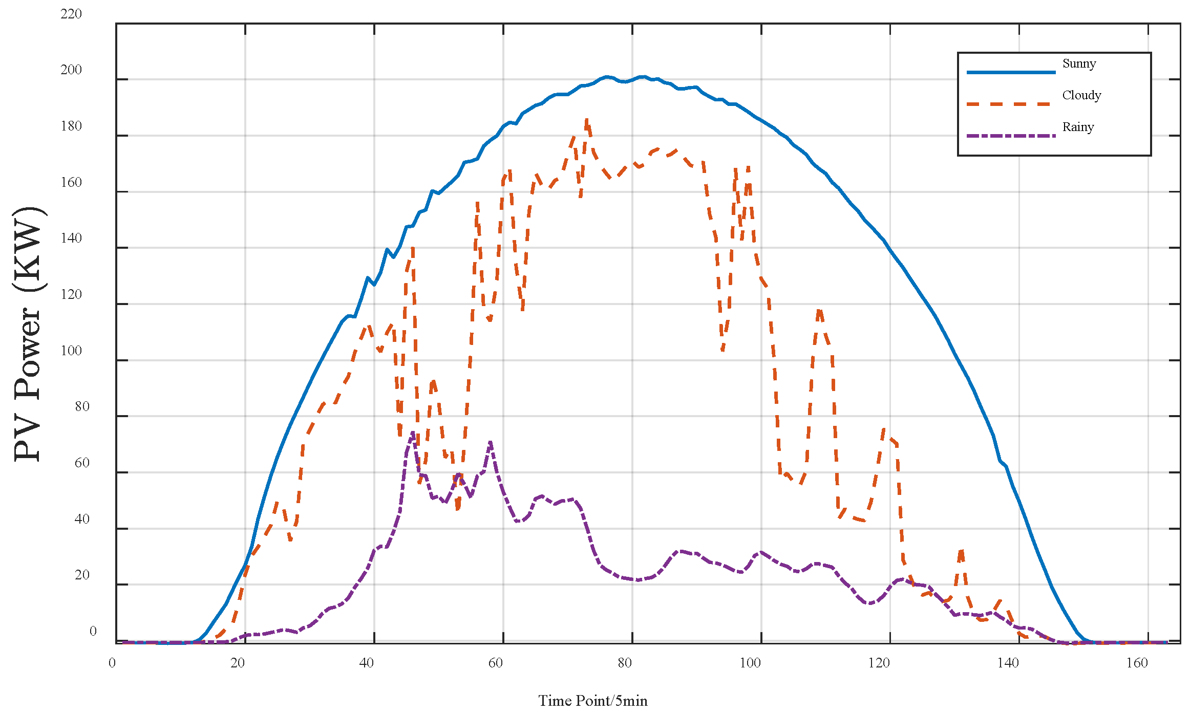
Using historical power data, the seasonal and weather distribution of PV power is analyzed, and prediction models are established for various seasons to improve the prediction accuracy.
The remainder of this work is organized as follows: Section 2 introduces the related methodologies including the RVM and SSA. Section 3 describes the proposed SSA-RVM method and presents the forecasting model based on the SSA-RVM in detail. Section 4 conducts the numerical experiments, and the results are discussed. Finally, conclusions are presented in Section 5.

2. Methodology

The RVM and SSA are the footstones of this work, and the basic theories of them will be briefly reviewed in this section.

2.1. Relevance Vector Machine

The RVM as a sparse probabilistic learning model is developed under the Bayesian framework combining Markov property, automatic relevance determination, and maximum likelihood theory. Given a data set of input–target pairs x n , t n n = 1 N , where x n is the input vector, t n is the target value, N is the total number of samples, the RVM regression model is defined as:
t n = i = 1 N w i K x , x i + w 0 + ξ n
where w i i = 1 , , N is the weight parameter, ξ n is the zero-mean Gaussian noise with a variance σ 2 , and K x , x i denotes a kernel function.
Under the independence assumption of t n , the likelihood estimation of the training set x n , t n n = 1 N can be written as:
p t | w , σ 2 = 2 π σ 2 N 2 exp ǁ t Φ w ǁ 2 2 σ 2
where t = ( t 1 , t 2 , t n ) , Φ = [ ϕ 1 ( x ) , , ϕ N ( x ) ] T , and ϕ i ( x ) = K x , x i represents a nonlinear basis function, The maximum likelihood estimation of w and σ 2 obtained directly by (2) may usually cause overfitting if no constraint is placed on weights w . To avoid this issue, the sparse Bayesian principle is commonly used to assign zero-mean Gaussian prior distribution to w as:
p ( w | α ) = i = 0 N N w i | 0 , α i 1
where α denotes hyperparameters with dimensions N + 1 . Consequently, each weight is assigned to a hyperparameter that may be used to control the impact of the prior distribution on each parameter and maintain the sparsity of the RVM model.
According to Bayesian rule, the posterior over all unknowns can be expressed by
p w , α , σ 2 | t = p t | w , α , σ 2 p w , α , σ 2 p ( t ) .
Then, given a new test point x , the predictions of related target in terms of predictive distribution can be obtained by:
p t | t = p t | w , α , σ 2 p w , α , σ 2 | t d w d α d σ 2
According to the definition of the prior probability distribution and likelihood distribution using the Bayesian principle, the posterior probability distribution of all unknown parameters can be calculated by
p w | t , α , σ 2 = p t | w , σ 2 p w | α p t | α , σ 2 = ( 2 π ) N + 1 / 2 | Σ | 1 / 2 exp { 1 2 ( w μ ) T Σ 1 w μ }
where Σ = σ 2 Φ t Φ + A 1 is the posterior covariance with A = d i a g α 0 , α 1 , , α N , and μ = σ 2 Σ Φ T t denotes the mean value.
To obtain the weight of the model, the optimal value of the hyperparameters should be computed first by the following iterative formulation.
α i n e w = γ i μ i 2
σ 2 n e w = ǁ t Φ μ ǁ 2 N i = 0 γ i
where μ i denotes the i th element of the μ ; γ i = 1 α i i i , where i i is the i th diagonal element of the posterior weight covariance Σ , which is calculated by the values of the parameters α and σ 2 .
Then, given a new input value x , we can obtain the probability distribution of the corresponding output as:
p t | t , α M P , σ M P 2 = p t | w , σ M P 2 p w | t , α M P , σ M P 2 d w = N t | y , σ 2
y = μ T φ x
σ 2 = σ M P 2 + ϕ x T Σ ϕ x
where y denotes the predicted mean, which is regarded as the predicted value t , and α M P and σ M P 2 stand for the maximum of the α and σ 2 , respectively.
To this end, the theory of the RVM has been introduced, and it shows strong generalization ability, good learning ability, flexible kernel function selection, simple parameter setting, and so on [35]. In addition, some outstanding properties of the RVM can be summarized as follows:
(1)
The RVM can be used not only for single-point but also for probability prediction;
(2)
Unlike the SVM, the choice of kernel function of the RVM may not satisfy Mercer’s theorem;
(3)
The penalty factor does not need to be set for the RVM. Only the kernel function parameters are set, which significantly simplifies the training process;
(4)
The RVM has sparsity characteristic, i.e., the number of relevance vectors in the RVM is less than that of the support vector in the SVM;
(5)
For unlearned samples, the generalization ability of the RVM is better than the SVM on the whole.
As mentioned above, the RVM can be used as a competitive candidate for PV power prediction. However, some hyperparameters significantly impact the performance of the RVM, and thus selecting the optimal parameters is a crucial problem to ensure superior prediction accuracy. Consequently, the SSA will be presented in the following subsection, which will be used to optimize the free parameters of the RVM.

2.2. Sparrow Search Algorithm (SSA)

According to the foraging and antipredation behaviors of sparrows, Xue proposed a new swarm intelligence optimization algorithm called the SSA in 2020 [41]. The SSA has a strong global search ability, good stability, and a quick convergence rate. It is not restricted by the objections of function differentiability, derivability, or continuity. The rules of sparrow behavior are usually assumed as follows [45,46,47].
(1)
The producer and the scrounger are two types of sparrows in the population. The root mean square error (RMSE) is commonly used as the fitness function during the RVM training process, and a smaller fitness value of the sparrow means that it has a richer energy store. The main task of producers is to find areas where food is abundant and to guide whole scroungers into the foraging areas.
(2)
When the predator is selected by the sparrow, the individuals start chirping as warning signals. Once the warning value exceeds the safety level, all scroungers are led by the producers to a safe area for foraging.
(3)
With each iteration, the identities of the producer and the scrounger change. Their identities can be switchable, and the scroungers with more resources can become the producers. In order to get a better position, the scroungers and producers have to change their position and swap their identities constantly, but the proportion of the two to the total population remains the same.
(4)
The fewer the scrounger’s resources, the worse his position in the population. It is easier to travel to other areas to obtain resources;
(5)
During a group search, the scrounger will always surround the producer, forage in the vicinity of the producer, and compete with the producer for resources.
The position of the sparrow can be written as the following matrix:
X = x 1 , 1 x 1 , 2 x 1 , d x 2 , 1 x 2 , 2 x 2 , d x n , 1 x n , 2 x n , d
where x n , d is the d dimensional position of the nth sparrow, and n denotes the number of sparrows.
The fitness value of all sparrows can be defined as:
F X = f x 1 , 1 x 1 , 2 x 1 , d f x 2 , 1 x 2 , 2 x 2 , d f x n , 1 x n , 2 x n , d
where n is the number of sparrows, and the value of each row in F X denotes the fitness value of the individual, reflecting the energy reserve.
In the optimization process of the SSA algorithm, the producers with higher energy storage are given priority when searching for food. Because the producers provide the foraging search direction for the whole population, the producer has a larger search range than the scroungers. In the iterative process, the location of the producer is updated as below:
X i , j t + 1 = X i , j t exp i α i t e r max i f R 2 < S T X i , j t + Q L i f   R 2 S T
where t denotes the current iteration, j = 1 , 2 , , d , X i , j t represents the value of the j th dimension of the i th sparrow at iteration t , and i t e r max is a maximum number of iterations. α ( 0 , 1 ] is a random number. R 2 represents the warning value, and S T indicates the safety threshold. Q is a random number that follows the normal distribution. L indicates a matrix of 1 × d for which each element inside is 1. R 2 < S T means that no predators no predator is found within the safe range and can continue to forage for the optimal solution. Contrastingly, R 2 S T represents that some individuals detected predators and started to alert other sparrows. The population changed to the antipredation mode and moved to a safe area as soon as feasible.
The formula for updating the location of the scrounger is as follows:
X i , j t + 1 = Q exp X w o r s t t X i j t i 2 i f i > n / 2 X P t + 1 + X i , j t X P t + 1 A + L o t h e r w i s e
where X P denotes is the position of the individual with the best fitness value in the population. X w o r s t is the worst position of individuals in the current population. A is a matrix of 1 × d such that each element inside is randomly assigned 1 or 1 and A + = A T A A T 1 . When i > n / 2 , it shows that the i th scrounger with the low fitness value is most likely to be in a state of starvation. For the whole population, some sparrows serve as the detection and early warning function and are responsible for diffusing the warning signal to the entire population to lead the population to a new safety area. Sparrows accounting for 10% to 20%of the total population in each generation are randomly selected to perform the early warning function, and their position update formula is:
X i , j t + 1 = X b e s t t + β X i , j t X b e s t t i f f i > f g X i , j t + K X i , j t X w o r s t t f i f w + ε i f f i = f g
where X b e s t is the present global best position. β denotes a control parameter for the step size and is a standard normally distributed random number with a mean value of 0 and a variance of 1 . K [ 1 , 1 ] is a uniform random number. Here, f i is the fitness value of the present individual. f g and f w are the present global best and worst fitness values, respectively. ε signifies the smallest constant for avoiding zero-division error. f i > f g denotes that the sparrow is not in the center of the group and is in a marginal position. X b e s t represents a position in the center of the group and is safe in its surroundings. If f i f g , Sparrows in the middle of the population are aware of the threat and approach closer to other sparrows in the population to avoid being predated. Figure 1 shows the flow chart of the algorithm.

3. PV Power Forecasting Model via the SSA-RVM

In this section, a novel SSA-optimized RVM model, called SSA-RVM, will be proposed by incorporating the SSA into the RVM first. Second, we describe the PV power forecasting model based on the SSA-RVM.

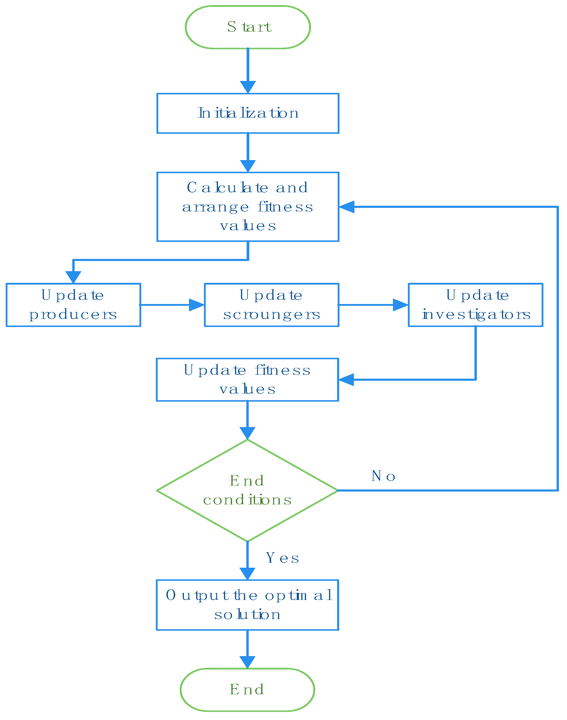
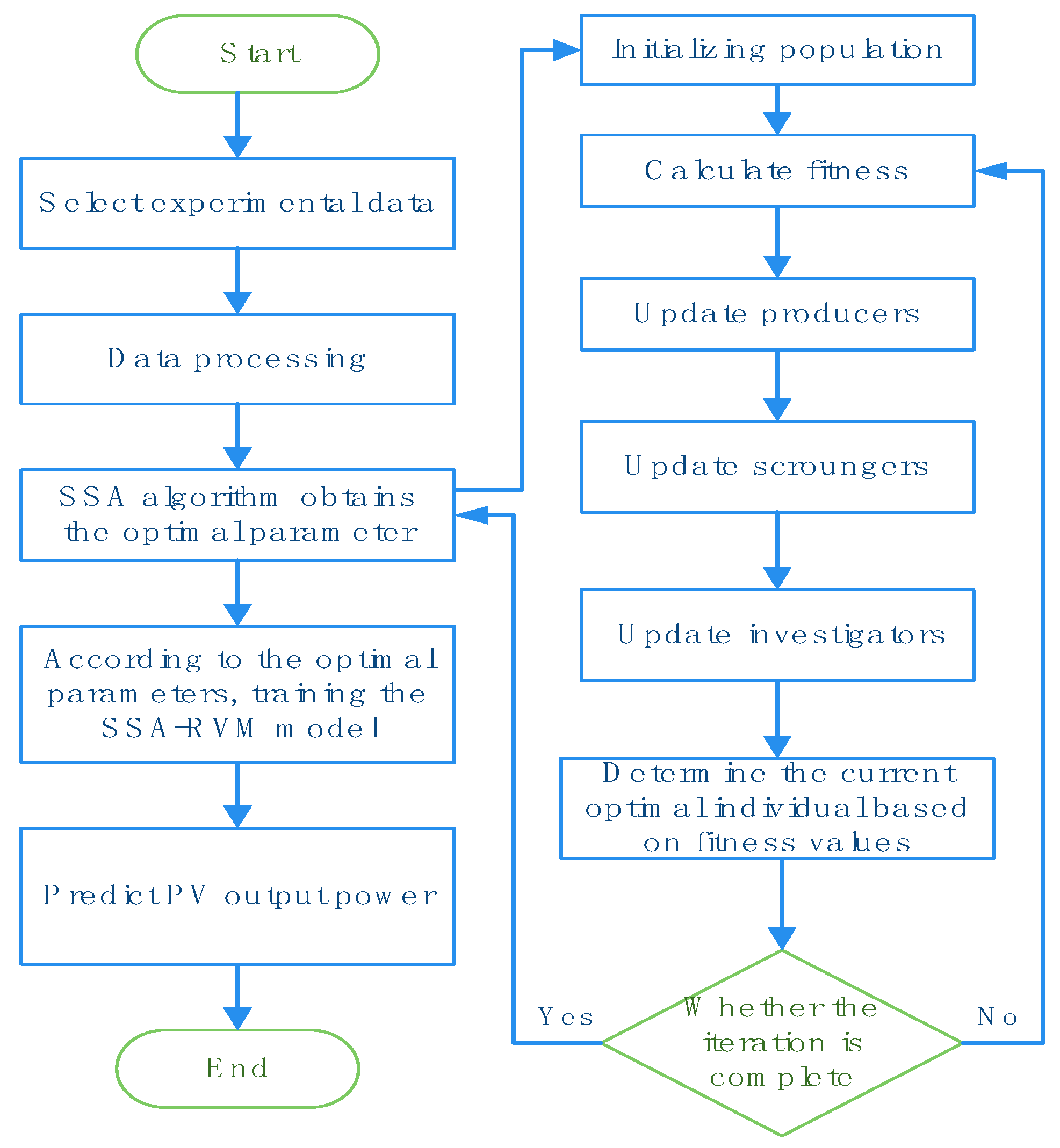
3.1. SSA-Optimized RVM (SSA-RVM)

The appropriate kernel function and suitable kernel width size have a critical impact on the performance of RVM regression. This research employs SSA to optimize the RVM to find the appropriate bandwidth parameter of training samples to enhance the RVM’s regression ability and increase its prediction performance.
The RVM algorithm realizes nonlinear mapping between data space and feature vector space through kernel functions in the learning process, and a good fitting can be obtained by choosing a suitable kernel function. A Gaussian kernel function with good distribution characteristics is selected in this paper, which has the advantages of good locality, fewer parameters, and less computation. The Gaussian kernel function has the following expression:
K x , y = exp ( x y ) 2 2 σ 2
where σ is the kernel width. The SSA algorithm is utilized to search for the optimal parameters of the RVM model for the best PV power forecasting performance, and the optimal procedure can be summarized in the following steps:
(1)
Select experimental data.
(2)
Set the parameters of the SSA algorithm: ST = 0.6 (the early warning value), SD = 0.2 (the number of the sparrows who perceive the danger), PD = 0.7 (the number of the producers); the initial parameters of the RVM model: α = 0.1; σ = 1.
(3)
Initialize the individual positions of the population in the SSA algorithm by calculating the fitness function to determine the current optimal individual and the optimal global individual.
(4)
Starting the iteration.
(5)
The optimal parameters are output if the constraint is met; otherwise, the iteration continues.
(6)
Establish and train the SSA-RVM model.
(7)
The prediction experiment is carried out with the SSA-RVM model.
(8)
End the program.
The process of parameter optimization by the SSA can be seen in Figure 2.

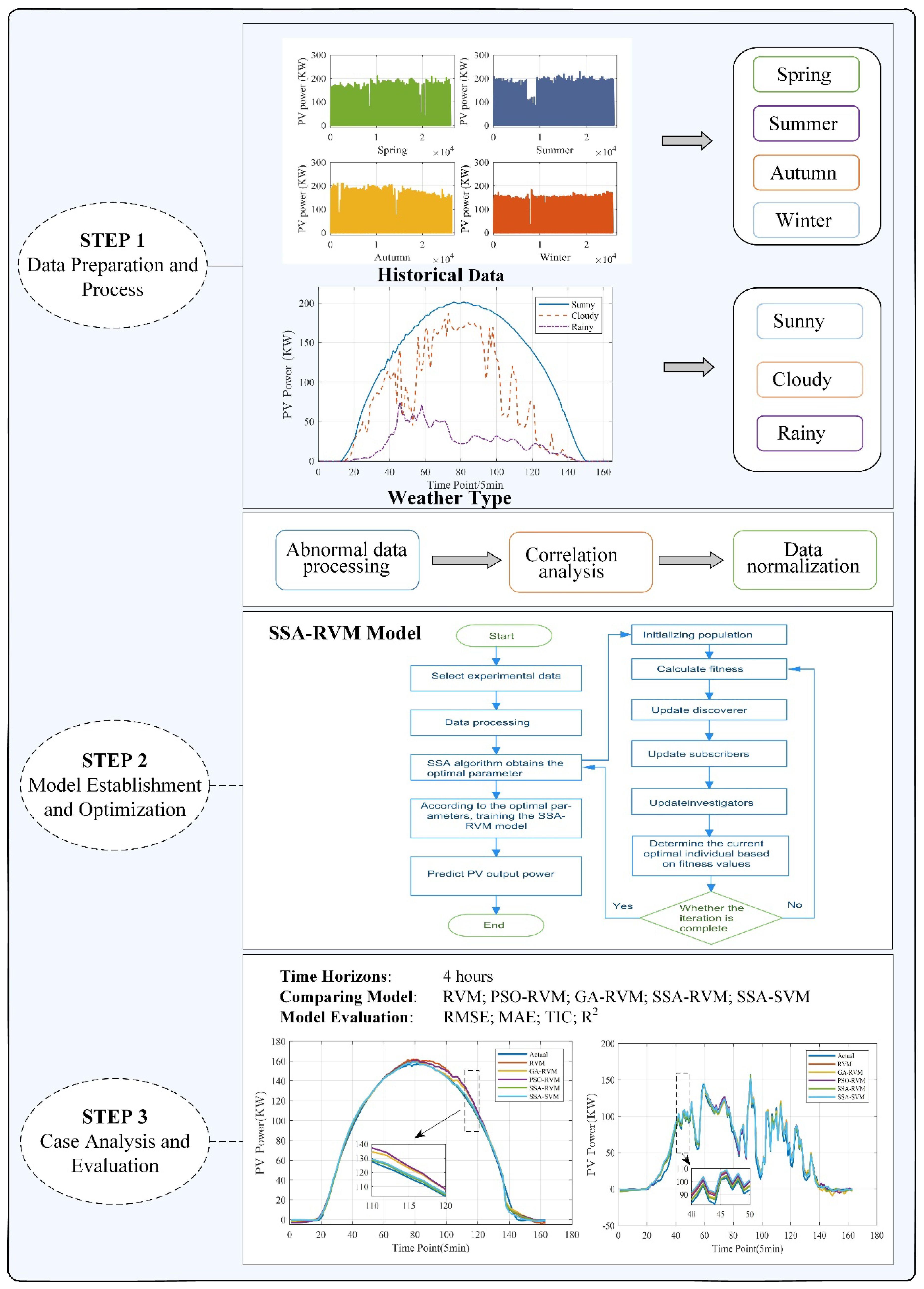
3.2. SSA-RVM-Based Forecasting Model

This subsection will present the PV power forecasting model by using the proposed SSA-RVM method.
(1)
Source and type of dataset
The data set from the “Desert Knowledge Australia Solar Center” is mainly used to evaluate the performance of the proposed SSA-RVM, which can be openly accessed at the URL http://dkasolarcentre.com.au (accessed on 10 January 2021). The data set used in this paper includes the daily PV power data with a 5 min time resolution from 5:00 to 19:30 every day from 1 January to 30 December, 2017, and meteorological data containing temperature, global horizontal radiation, diffuse horizontal radiation, wind speed, and wind direction. In the next experiment, data from four months are chosen and spread out over four seasons.
(2)
Analysis of influencing factors
PV power generation is nonlinear and stochastic in nature, and many influencing factors will lead to the variation of PV power. The influencing factors usually include internal factors and external factors. The internal factors mainly comprise aging of PV power plant equipment, loss during the energy transmission process, inverter performance, etc, while PV power is mainly influenced by the external environment, such as solar irradiance, temperature and humidity, weather, and season type. Considering the influence of various factors, the output power of a PV array can be expressed as:
P p V = η p V S I [ 1 0.005 ( t 0 + 25 ) ]
where η is the conversion efficiency of the solar cell panel, S denotes the area of the PV cell, I represents the solar radiation intensity, and t 0 stands for the operating temperature of the PV module. Assuming that the solar cell panel conversion efficiency and PV cell area are constant, the solar irradiation intensity and temperature will affect the power value.
(3)
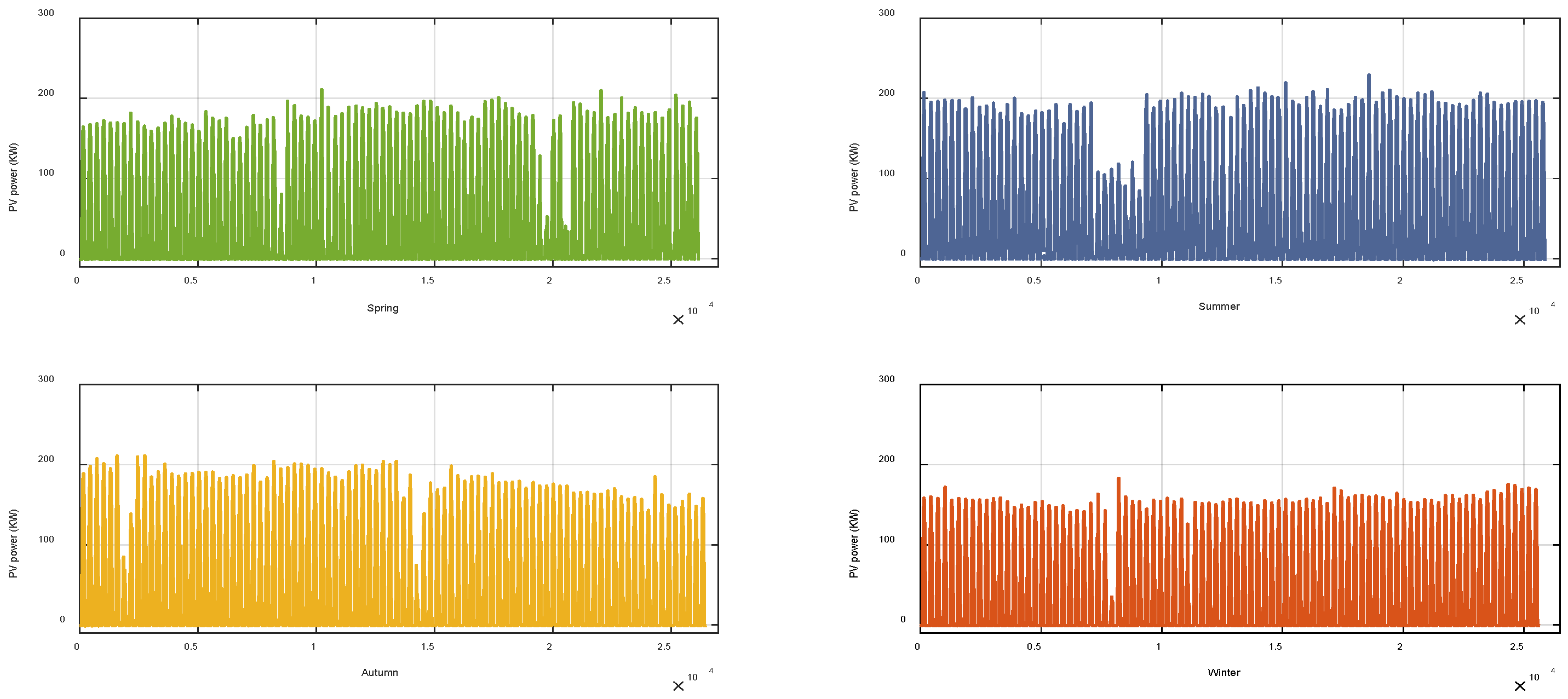
Seasonal distribution and weather types characteristics of PV output
Meteorological statistics, such as solar irradiance and atmospheric temperature, vary by season and weather type. The seasons have a substantial effect on the power output of PV arrays, even when temperature, humidity, and other meteorological variables (wind speed, wind direct) are excluded. The angle between the sun and the ground and the direct irradiance received by the PV panels vary throughout the year, resulting in seasonal variations in PV power output. Figure 3 illustrates the seasonal profile of PV power generation based on climate data. Summer has the largest total PV power generation, while winter has the lowest. The variance between winter and summer is relatively minor.
This paper selected a day with different weather types (including sunny, cloudy, and rainy) for the comparative analysis of the actual PV power. Figure 4 picks three days with different types of weather, and one can see that PV power is relatively stable and large in sunny weather, which shows strong regularity. Correspondingly, PV power is not as stable as on sunny days due to cloud cover in cloudy weather. It is clear that the PV power is relatively small, fluctuating, and less regular in extreme rainy weather.
(4)
Correlation analysis of influencing factors
As aforementioned, various factors influence PV power. Selecting the key factors can avoid redundant information and reduce the complexity of the model. To choose the appropriate influencing factors, this paper analyzes the correlation relationship between various factors and PV power generation using the Pearson correlation coefficient (PCC) method. To further verify the correlation degree, the maximum information coefficient (MIC) (suitable for linear and nonlinear problems) is also used to analyze the correlation degree between many factors and PV power. The PCC is defined as:
r x , y = i = 1 n x i x ¯ y i y ¯ i = 1 n x i x ¯ 2 i 1 n y i y ¯ 2
where x = ( x 1 , x 2 , , x n ) and y = ( y 1 , y 2 , , y n ) are two vectors with the same dimensions, and x ¯ and y ¯ denote their average value, respectively. The value range of r x , y is [−1, 1]. When y increases with the increase in x , the trend of change increases and decreases with the same positive correlation; otherwise, it is a negative correlation. The size of the absolute value of the correlation coefficient will reflect the level of the correlation between y and x .
As another essential nonlinear correlation evaluation criterion, the MIC is defined as:
M I C ( x ; y ) = max a × b < B I ( x ; y ) log 2 min ( a , b )
where a , b is the number of grids divided in the direction, which is essentially the grid distribution, and B is a variable. The higher the similarity, the greater the value, and vice versa.
The correlation between the influencing factors and the output power can be calculated using the above two formulas. The correlation results of PCC and MIC are shown in Table 1.
It can be seen from the results in Table 1 that the global horizontal radiation (GHR), diffuse horizontal radiation (DHR), Weather Temperature Celsius, and weather relative humidity and moderation have a significant influence on PV power generation. Therefore, these factors can be identified as the input vectors of the model.
In addition to external weather influencing factors, the information of historical power data must also be considered for the output of PV power. This paper determines the input sequence length of historical power data through autocorrelation analysis to obtain better model accuracy and a more concise model structure. The autocorrelation coefficient (ACC) with a lag of h is given by:
r h = i = 1 n 1 x i x ¯ x i + h x ¯ i = 1 n x i x ¯ 2
where x ¯ denotes the mean value of the x variable, and h is the time lag. The length of the historical input power is judged by analyzing the autocorrelation of the historical power, and the results of the autocorrelation calculation are given in Table 2. According to the results, we know that ten historical power points have an autocorrelation bigger than 0.6, and hence the embedded dimension of the historical power is set at ten.
According to the preceding analysis, the input vector-matrix can be written as X = [ I G H , I D H , I W T , I W H , Y H 1 , Y H 2 , Y H 10 ] , where I G H , I D H , I W T , I W H are the measured values of GHR, DHR, WTC, and WRH for the time to be predicted, respectively. Y H 1 , Y H 2 …… Y H 10 are historical power data.
(5)
Data Processing and Evaluation Indexes
Data processing includes abnormal data preprocessing and data normalization. Abnormal data processing refers to deleting anomalous data or smoothing. In this paper, the range of the maximum and minimum values is counted, the reasonable range of all data values is determined, and the obvious abnormal data are dealt with by deleting and taking the mean value before and after. For the collected historical power data and meteorological data, there is usually a large gap between the feature vectors in the data. To avoid the problem of a slow learning rate caused by different data dimensions and promote the performance of the prediction model, the normalization process is usually utilized to the original data to the range of [0, 1] by
x ˜ i = x i x min x max x min
where the normalized value is x ˜ i , x i represents the original data, x max indicates the maximum value of the original data, and x min is the minimum value of the original data.
In this work, four evaluation indexes are primarily employed to evaluate the performance of the proposed prediction model, which are defined as follows.
  • Root Mean Square Error (RMSE)
RMSE = 1 n i = 1 n y ^ i y i 2
  • Mean Absolute Error (MAE)
MAE = 1 n i = 1 n y ^ i y i
  • Theil Inequality Coefficient (TIC)
TIC = 1 n i = 1 n y ^ i y i 2 1 n i = 1 n y i 2 + 1 n i = 1 n y ^ i 2
  • R-Squared (R2)
R 2 = 1 i = 1 n y i y ^ i 2 i = 1 n y i y ¯ 2
where y i denotes the real power value, y ^ i is the predicted power value, y ¯ represents the mean value of the real value, and n denotes the size of the evaluation data set.
(6)
Forecasting Model based on SSA-RVM
According to the data analysis and pretreatment above, the primary modules of the forecasting model using the SSA-RVM are composed of data preprocessing, construction of the SSA-RVM, and prediction result analysis and evaluation module. The overall processes of PV power prediction via the model described in this paper are summarized in the following steps.
Step 1: Data preparation.
Step 1.1: Divide the PV output historical data according to the seasons and weather type.
Step 1.2: Data preprocessing and correlation analysis of influencing factors.
Step 2: Establish the forecasting models.
Step 2.1: Use the SSA-RVM model to set up and improve the forecasting models for each season.
Step 3: Case analysis and evaluation.
Step 3.1: Predict the PV power generation of different weather types in different seasons.
Step 3.2: Compare the other prediction models and evaluate the results.
The detailed framework of the proposed model is given in Figure 5.

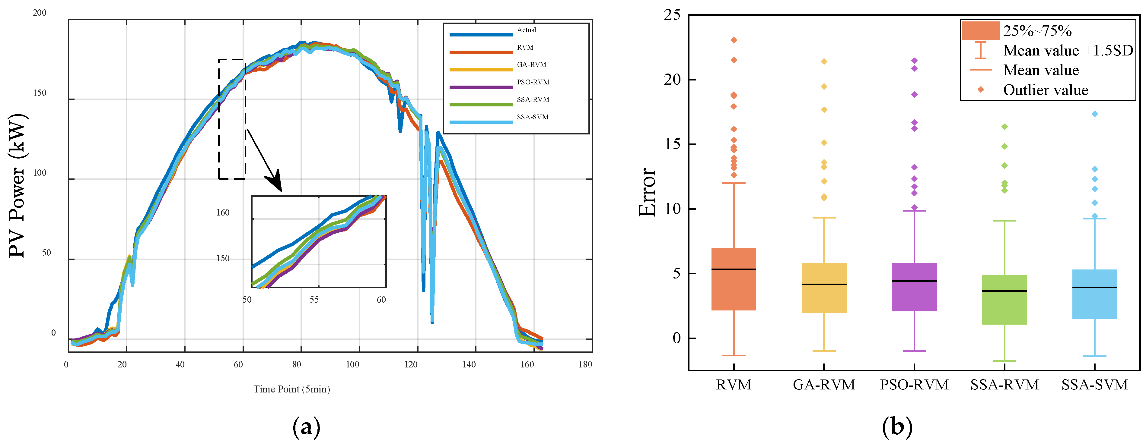
4. Results and Discussion

Some experiments are carried out in this section to verify the performance of the proposed SSA-RVM forecast model under different cases. Section 3.2 describes the data source used in the experiment (Desert Knowledge Australia Solar Center) and detailed data information (data from 5:00 to 19:30 every day in 2017, with a time resolution of 5 min). The detailed implementation procedure of the PV power prediction system with the SSA-RVM model is depicted in Section 3.2 According to the geographical location of the PV power stations (Section 3.1) selected in this paper, the four seasons are as follows: spring is September–November, summer is December–February, autumn is March–May, and winter is June–August. Models are constructed separately for four seasons: one month of data is selected for each season to conduct experiments. January data are selected in summer, April in autumn, July in winter, and September in spring. The data selected for each month are randomly arranged by day, the data of the first 25 days in summer and winter are selected as the training set, and the remaining 6 days are used as the test set. The data for the first 25 days in the spring and autumn seasons are selected as the training set, and the data for the remaining 5 days are used as the test set. Predict the PV power under different weather types each season, and the prediction time scale is 4 h. The RVM, PSO-RVM, GA-RVM, and SSA-SVM are selected for comparison to test the performance of the SSA-RVM model. The PV power curves of different forecast methods under different weather types are compared.
In the following subsections, we conduct different experiments on the Matlab 2017b platform with a computer of Intel Core i5, 2.60 GHz CPU, and a 64-bit Win10 system.

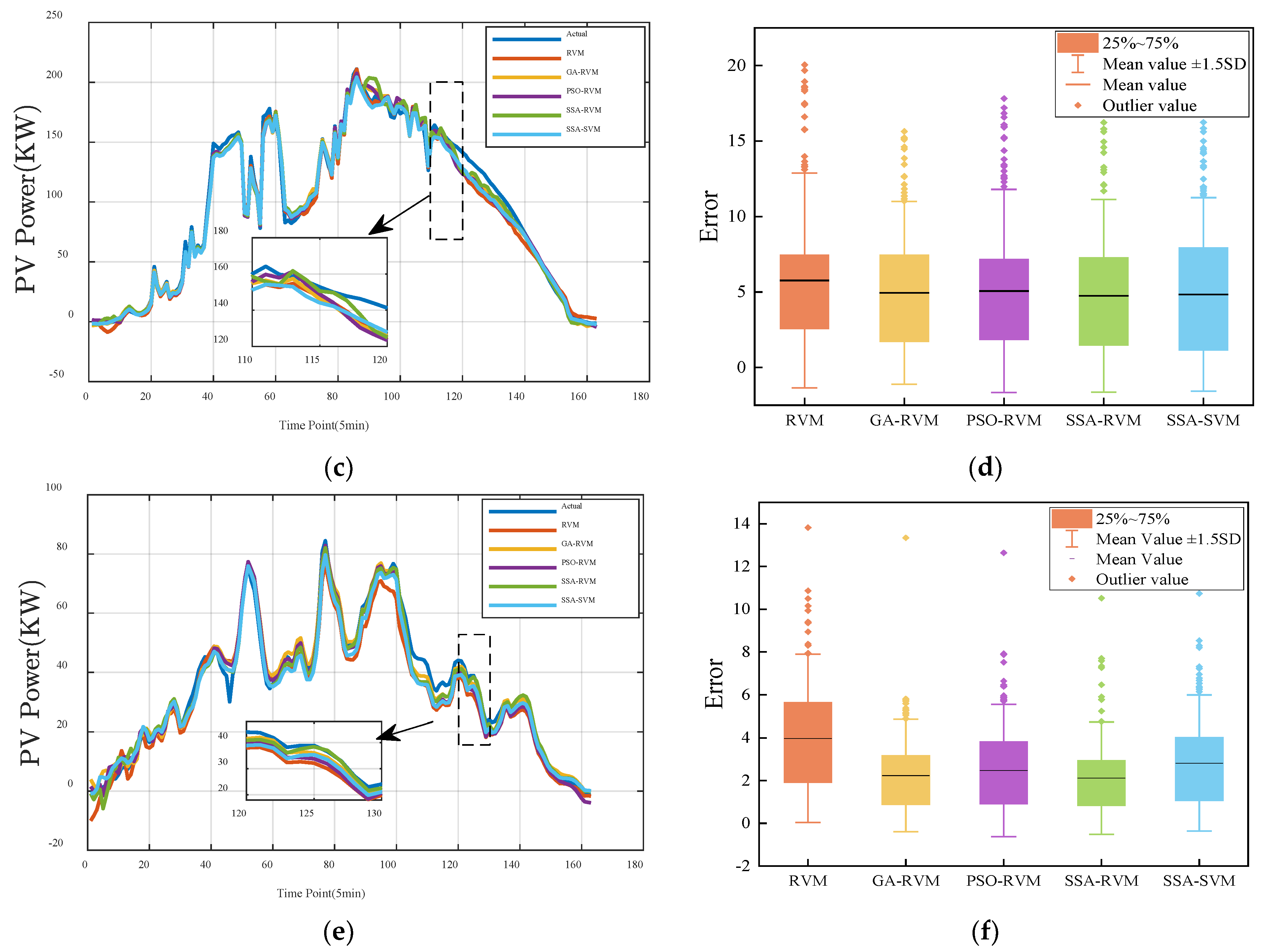
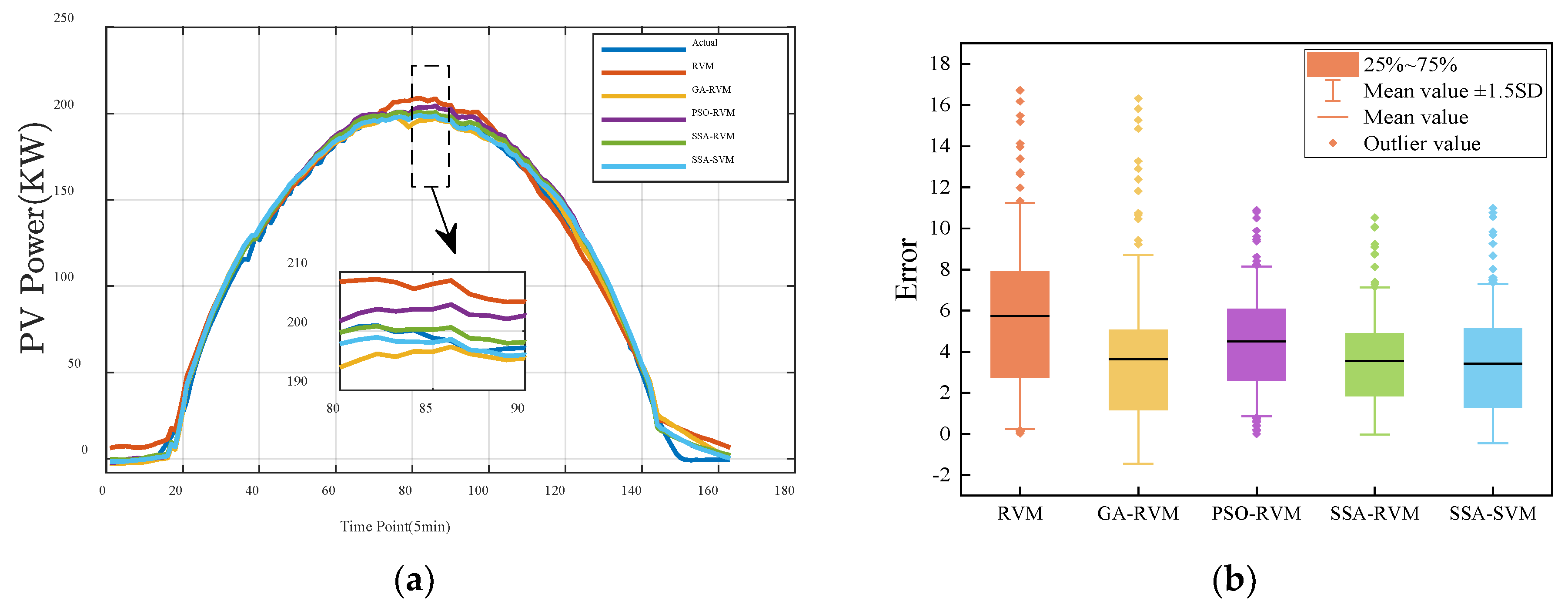
4.1. Forecasting Results in Summer

This subsection performs experiments to test the accuracy of the proposed method under different weather types (including sunny, cloudy, and rainy days) in summer. The prediction results are given in Figure 6, which includes the power prediction results curves of different models and the error analysis diagram. It can be seen from Figure 6a,c,e that the predicted trend of the five models is approximately the same as the actual values. In sunny weather, the PV power increases and decreases with time, and the fluctuation is slight. The PV power fluctuates obviously, and the power value is small in rainy weather. In three different weather types, one can see from Figure 6a,c,e that the predicted results of the proposed SSA-RVM model are all closest to the actual values, and the gap between the actual values and other models is more significant. The mean absolute error (MAE) results are given in Figure 6b,d,e, and one can see that the MAE of the proposed model SSA-RVM is the smallest, especially in rainy weather, with obvious advantages. Variations in various meteorological factors mainly cause this: under sufficient sunshine conditions, PV output power changes slowly with light intensity and atmospheric temperature, while under insufficient sunshine, the PV output power changes rapidly with the meteorological factors.
Table 3 gives the results of the different evaluation indexes of several prediction methods under different weather conditions. From the results in the table, one can also know that the prediction accuracy of PV power in different weather is slightly different, and the prediction effect in rainy weather is slightly worse than that in sunny weather. However, the predicted results of the RVM model are delighted. R2 (the larger, the better) values are all around 0.99 in sunny weather, and the effect is relatively worse on rainy days, but R2 values also reach above 0.95. Among them, the SSA-RVM model proposed in this paper is superior to other models: in three weather conditions, R2 is above 0.99, and TIC (the smaller, the better) is below 0.04, which shows that the prediction effect is excellent.
In sunny weather: Compared with the traditional RVM model, the RMSE of the SSA-RVM model is reduced by 1.8009 kW, about 25.97%. MAE decreased by 1.1654 kW, about 1.44%, and R2 increased by 0.51%. Compared with the GA-RVM, PSO-RVM, and SSA-RVM models, RMSE decreased by 4.80%, 10.1%, and 2.8%, respectively, and MAE decreased by 12.25%, 17.57%, and 6.94%, respectively.
In cloudy weather: Compared with the traditional RVM model, the RMSE of the SSA-RVM model is reduced by 1.0915 kW, about 14.64%. MAE decreased by 1.017 kW, about 17.65%, and R2 increased by 0.40%. Compared with the GA-RVM, PSO-RVM, and SSA-RVM models, RMSE decreased by 0.15%, 5.80%, and 1.26%, respectively, and MAE decreased by 3.99%, 6.34%, and 1.90%, respectively.
In rainy weather: Compared with the traditional RVM model, the RMSE of the SSA-RVM model is reduced by 2.0119 kW, about 42.33%. MAE decreased by 1.875 kW, about 46.77%, and R2 increased by 3.19%. Compared with the GA-RVM, PSO-RVM, and SSA-RVM models, RMSE decreased by 3.31%, 14.64%, and 22.10%, respectively, and MAE decreased by 5.44%, 14.37%, and 24.96%, respectively.
The experimental results demonstrate that the proposed SSA-RVM-based prediction model has the best prediction effect for different weather types in summer, especially in rainy weather, and its performance is significantly better than the other models.

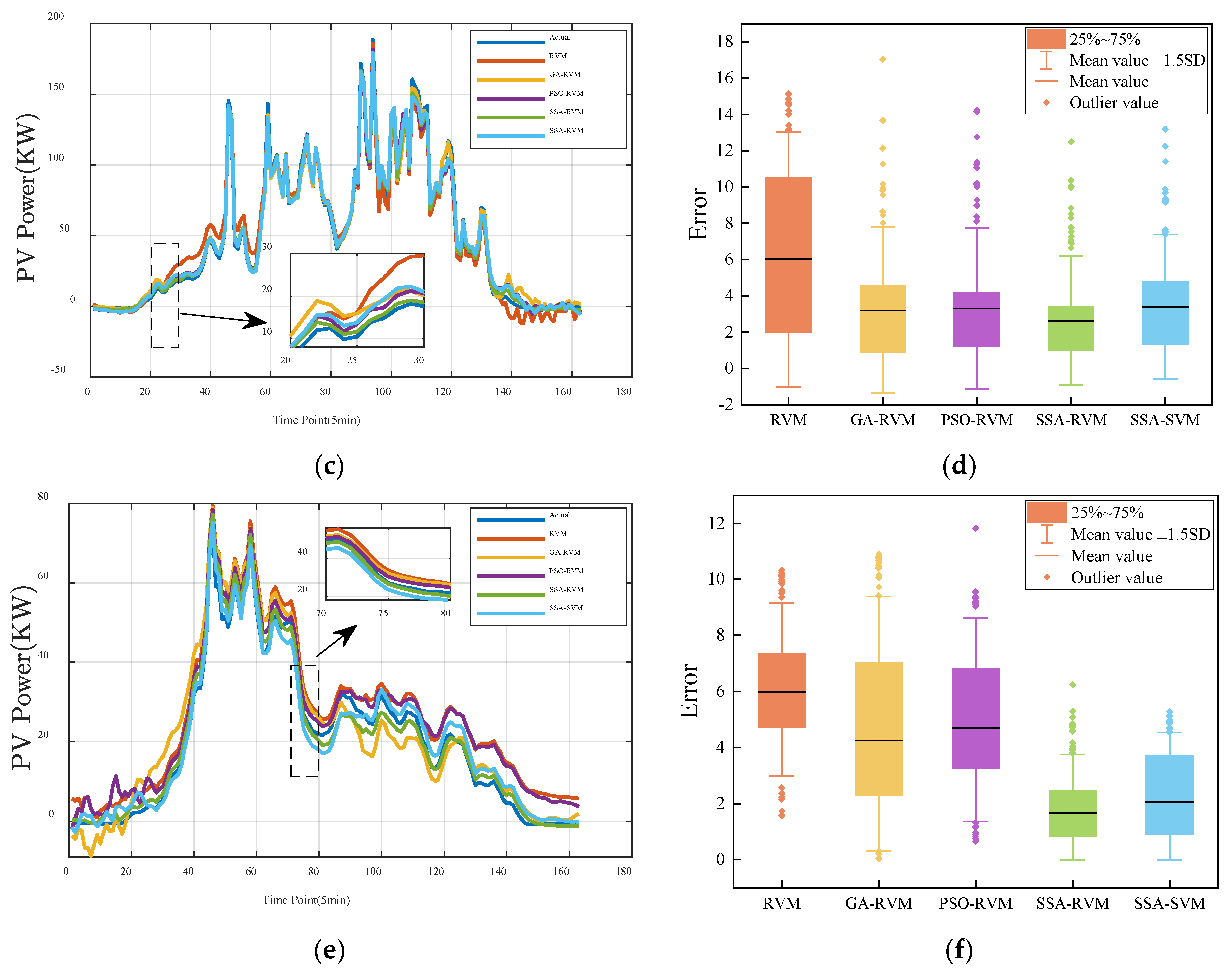
4.2. Forecasting Results in Autumn

Here, we further select the data with different weather types (including sunny, cloudy, and rainy days) in autumn to evaluate the forecasting performance of different methods. The forecasting results are shown in Figure 7. It is apparent from the figure that the fluctuation of PV output power is evident on rainy and cloudy days in this season, and it is relatively gentle on sunny days. From comparing power curves under sunny and cloudy weather, the prediction results of different models are close to the actual value. Still, under rainy weather, due to significant changes, the prediction curve of the SSA-RVM is the closest to the actual value, and others have an enormous difference. Compared with the predicted power of three weather types in summer, the fluctuation in rainy days in autumn is more evident because the weather conditions of the selected autumn training set are more complicated. From the error analysis (Figure 7b,d,e), one can observe that the mean absolute error of sunny and cloudy weather is similar, and the difference between rainy weather is obvious, which means that the SSA-RVM model significantly improves the prediction performance in rainy weather.
Table 4 gives the prediction evaluation indexes under different weather conditions this season. From the results in this table, the R2 of the proposed method reaches more than 0.98 on a sunny day and a cloudy day. The PV output power curve has a large fluctuation with weak regularity in rainy weather, but the R2 of rainy weather reaches more than 0.95, lower than sunny and cloudy weather.
The experimental results under different weather conditions in autumn also show that the prediction performance of the method proposed in this paper is available. It is consistent with summer. On a rainy day, the advantage of the prediction effect is more obvious.

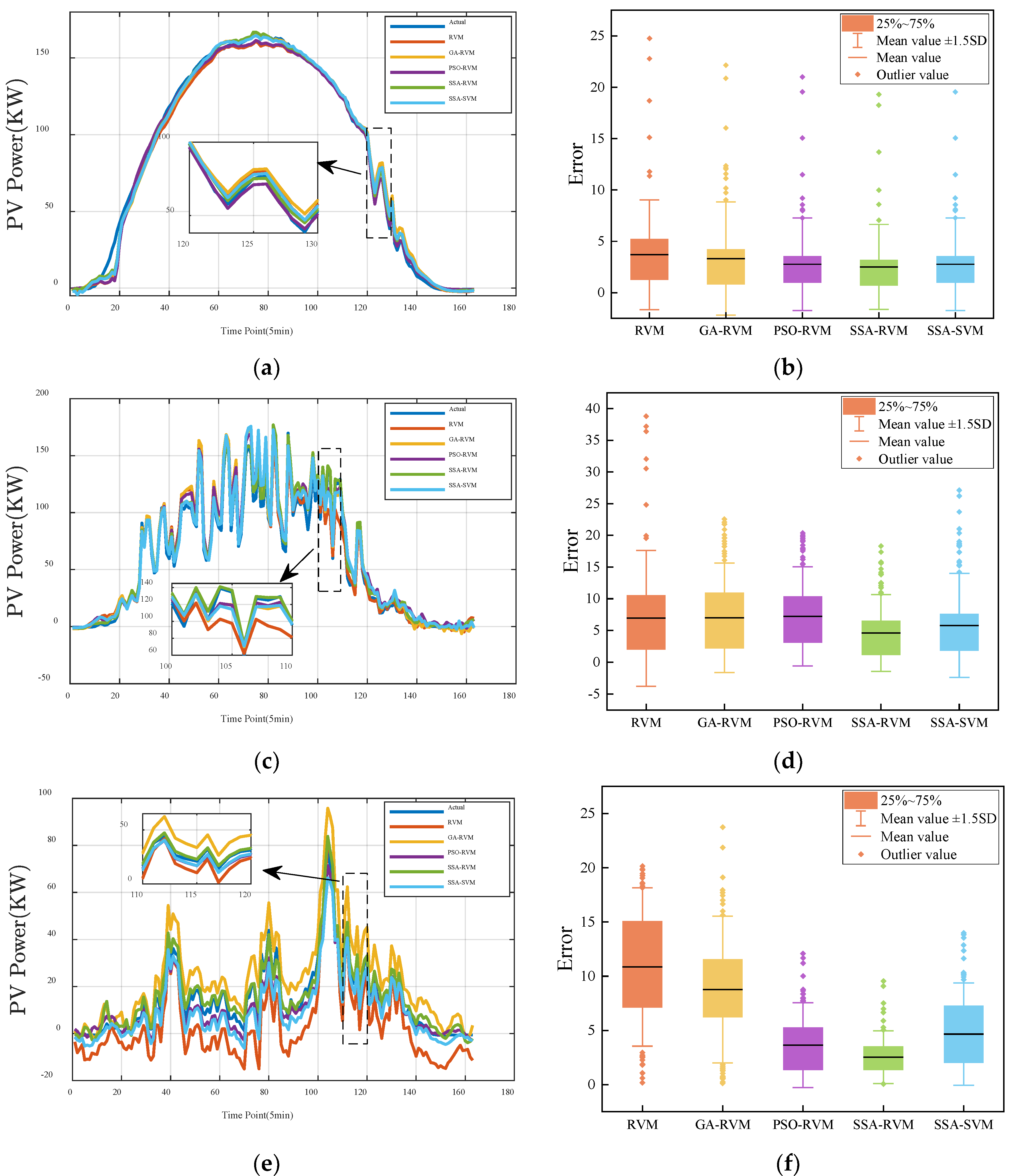
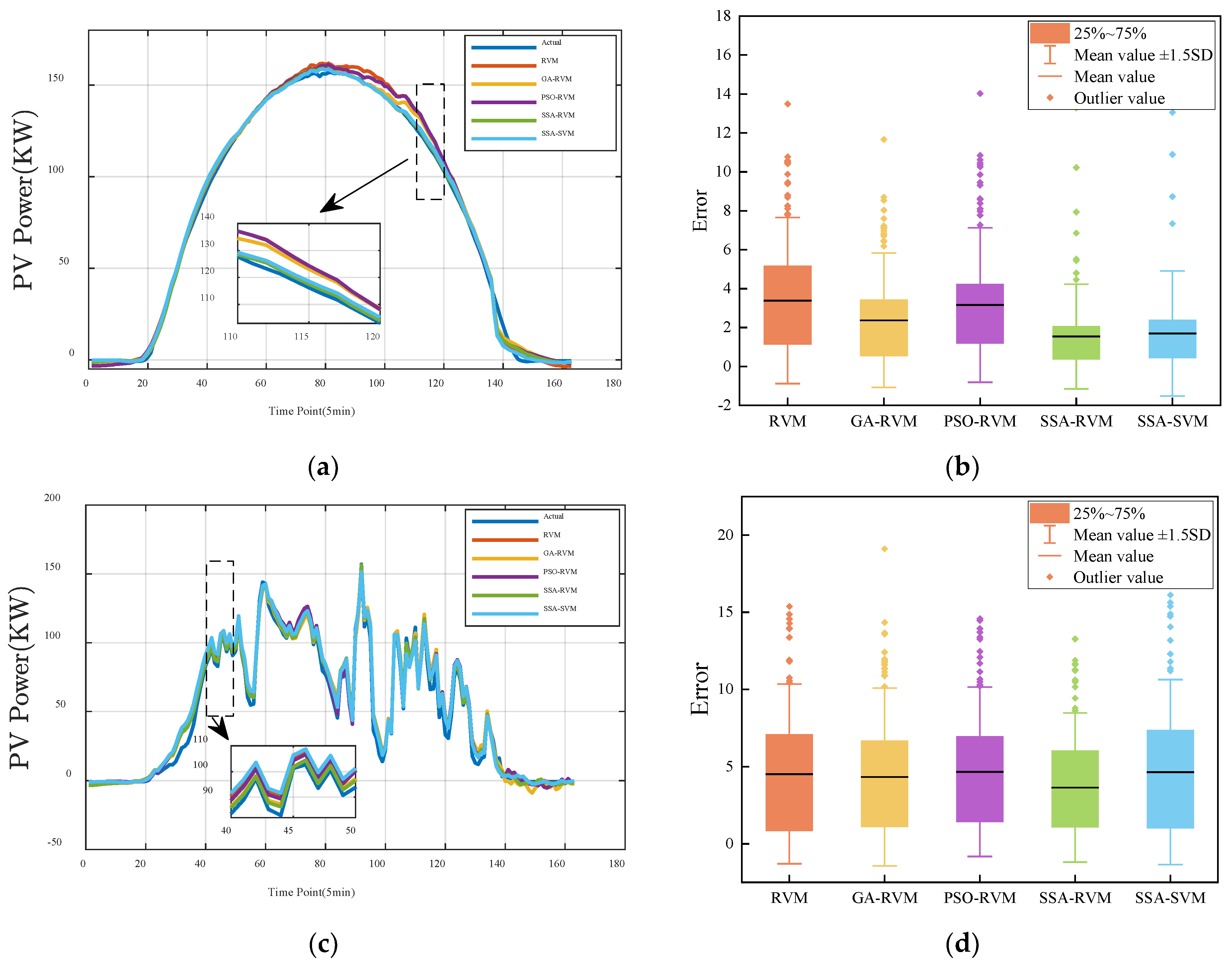
4.3. Forecasting Results in Winter

The predicted PV power curve in winter is shown in Figure 8. Compared with other seasons, the PV output power in winter is generally lower, and there is a small gap between the predicted and the actual results under various weather conditions. On sunny days, the fluctuation of PV output power is gentle. One can clearly see from Figure 8a that the prediction power curve of the GA-RVM and the PSO-RVM show noticeable fluctuation. The prediction curve of the SSA-RVM and the SSA-SVM is the closest to the actual value. Figure 8b shows the error. The mean value of the SSA-RVM is the lowest among other methods. From the comparison of power curves, under sunny and cloudy weather, the prediction results of different models are close to the actual value, but under rainy weather, due to significant changes, the prediction result of the SSA-RVM used in this paper is the closest to the actual value, and others have a larger difference. From Figure 8b,e,f, the mean value of the SSA-RVM method is lower, and the outlier value is less than the other methods.
As seen in Table 5, the SSA-RVM model still shows better prediction results than the other models under sunny, cloudy, and rainy days in winter, just like previous analyses of experimental results.
Experimental results demonstrate that the prediction effect of the proposed model is satisfactory under different weather types in winter, especially in sunny weather, because the power is flat and there is no fluctuation. The prediction result of the proposed model is very close to the actual value, and R2 is as high as 0.9985. As with the seasons analyzed above, the proposed model has a tremendous advantage under rainy weather, with its RMSE and MAE values reduced by about 1/3 compared with the traditional model.

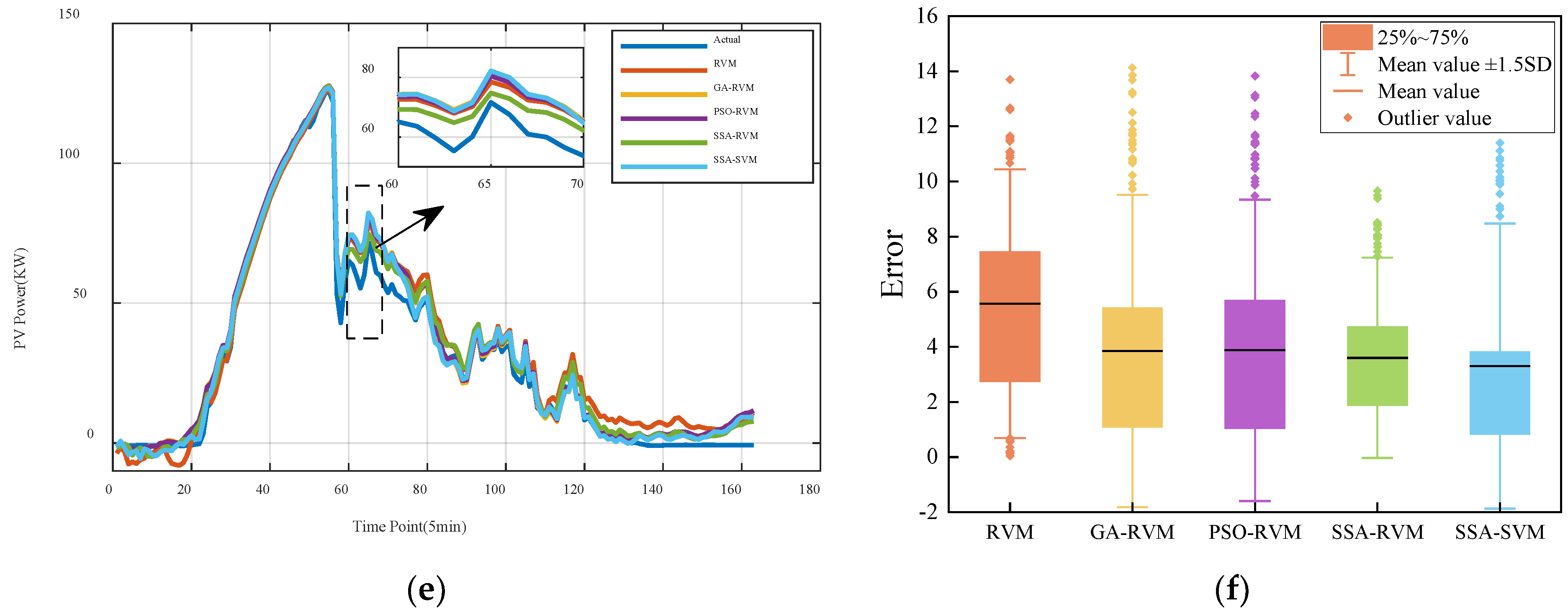
4.4. Forecasting Results in Spring

The prediction results under different weather conditions in spring are shown in Figure 9. Figure 9a shows that on sunny days, the predicted value of the traditional RVM model has a particular gap with the actual value, while the predicted value of other optimization models has a small gap with the real value, among which the predicted values of the SSA-SVM and the SSA-RVM are more close to the true value. As can be seen from error Figure 9b, the average absolute error of all models is relatively close, mainly because the weather fluctuation is slight on sunny days so that all models can get better prediction results. Under cloudy weather, the prediction result obtained by the proposed SSA-RVM is closest to the true value. On rainy days, fluctuations are very noticeable. In the error analysis figure, the mean absolute error of Figure 9f is lower than that of other approaches. Compared with the different seasons analyzed above, the difference between curves in Figure 9e is large. Since the experimental findings of the previous three seasons indicate that the SSA-RVM model has more significant advantages on rainy days, this model’s efficacy should be verified further. Compared with the other seasons, the training data selected by the model in this season lacks a certain amount of rain day data, resulting in unsatisfactory overall prediction results. However, in this case, the predicted value of the SSA-RVM model is still the closest to the actual value, which fully demonstrates the predictive ability of this method. The experimental results fully confirm that compared with other methods, the predicted value of the SSA-RVM is the closest to the actual value, fully demonstrating its advantage in different conditions.
Table 6 gives the error analysis of deterministic prediction results of several prediction methods in spring. In sunny weather, compared with other models, the RMSE is 3.7202, MAE is 2.5052, and R2 is 0.9966. In cloudy weather, the RMSE is 6.1017, MAE is 4.591, and R2 is 0.9872. In rainy weather, the prediction effect of other models is not satisfactory. Only the SSA-RVM model is significantly better than the other models. Compared with the traditional RVM, the RMSE is reduced by at least 74.76%, MAE is reduced by at least 76.69%, R2 is increased by 43.16%, and TIC is reduced by 77.61%. Compared with other optimization algorithms, the RMSE is reduced by at least 32.87%, and MAE is reduced by at least 30.34%. In rainy weather, the prediction effect of this model is greatly improved compared with other models.

4.5. Calculation Efficiency Analysis

Calculation efficiency is another key index to evaluate the feasibility of the prediction methods. In this section, we perform a calculation efficiency analysis of the developed model in terms of the number of the weight vector and the computing time under the experiments in Section 4.1.
From the above experimental analysis, the proposed SSA-RVM method has the best prediction effect, and the model with a slightly worse prediction effect than the SSA-RVM is the SSA-SVM. The biggest advantage of the RVM over the SVM is that it has better sparsity while ensuring better performance. In the RVM, the corresponding training data sample whose weight value (not zero) is called the“correlation vector”, and the sample data that determine the classification function in the SVM are called the “support vector”. The number of correlation vectors of the RVM and the number of support vectors of the SVM are given in Table 7. One can know from the results in Table 7 that the number of relevance vectors of the RVM is much less than that of the number of support vectors in the SVM, which means that the RVM has better sparsity than the SVM. In addition, the number of support vectors of the SVM is too large when the training sample is more prominent, which affects its decision-making speed. These results demonstrate that the RVM-based forecasting model has higher calculation efficiency than the SVM, which means that the proposed SSA-RVM with the same correlation vector as the RVM is suitable for PV power prediction.
Here, we further count the time consumption of different models depending on a computer with Intel Core i5, a 2.60 GHz CPU, and a 64-bit Win10 system. The training time is calculated at each iteration during the training stage, and the testing time is the processing time of all testing samples. The results of time consumption are given in Table 8. One can see from the results that (1) the traditional RVM performs faster than the optimized method in the training and testing stage because the optimization process takes some time. (2) The optimized RVMs consume more time than the traditional RVM, but the prediction accuracy of them is better than nonoptimized RVM, and thus the excessive time consumption is acceptable. (3) The testing time of the SSA-RVM model is faster than that of the SSA-SVM model, which shows that the decision-making speed of the RVM is faster than that of the SVM. (4) Compared with the PSO-RVM and GA-RVM models, the time consumption of the SSA-RVM is marginally superior, which shows the rapid convergence of the SSA. In addition, we see that the SSA-RVM has higher calculation efficiency than the SSA-SVM, which further demonstrates that the RVM is more efficient than the SVM. According to the analysis above, we know that the proposed SSA-RVM model is suitable for PV power prediction in practice.

5. Conclusions

In this paper, a novel parameter-optimized RVM via the SSA, named SSA-RVM, is developed for ultra-short-term PV power prediction application. In the proposed method, the SSA is utilized to improve the RVM accuracy by making use of the advantage of SSA and the superiority of the RVM. In addition, considering that the PV power has the characteristic of considerable fluctuations over time as well as seasonal distributions, and thus the prediction model via the SSA-RVM in different seasons is established to forecast the PV output power under different weather conditions. The simulation results show that the proposed SSA-RVM prediction model shows better prediction accuracy than the traditional support vector machine and RVM models. Furthermore, it is more suitable for ultra-short-term PV output prediction in practice considering the calculation efficiency.
The proposed SSA-RVM-based prediction model is used in the time domain space to forecast the PV power in this paper, and we will incorporate some decomposition methods, such as empirical mode decomposition (EMD) and variational mode decomposition (VMD), into the SSA-RVM model to further improve its accuracy in our future work. In addition, a stacked SSA-RVM may be studied for PV power ultra-short-term or long-term prediction to address the overfitting issue in the future.

Author Contributions

Conceptualization, W.M. and L.Q.; methodology, W.M. and L.Q.; software, L.Q.; validation, F.S. and S.S.M.G.; data curation, L.Q.; writing—original draft preparation, L.Q. and W.M.; writing—review and editing, W.M. and S.S.M.G.; supervision, J.D. and W.M. All authors have read and agreed to the published version of the manuscript.

Funding

This research was funded by the National Natural Science Foundation of China (Grant No. 61976175, 51877174), the Key Project of Natural Science Basic Research Plan in Shaanxi Province of China (Grant No. 2019JZ-05), the Key Laboratory Project of Shaanxi Provincial Education Department Scientific Research Projects (Grant No. 20JS109), and Guangxi Key Laboratory of Wireless Wideband Communication and Signal Processing. The authors also appreciate the support from Taif University Researchers Supporting project TURSP 2020/34, Taif University, Taif, Saudi Arabia.

Institutional Review Board Statement

Not applicable.

Informed Consent Statement

Not applicable.

Acknowledgments

The authors are grateful for the editor and the anonymous referees’ helpful comments on this paper.

Conflicts of Interest

The authors declare no conflict of interest.

References

  1. Elum, Z.A.; Momodu, A.S. Climate change mitigation and Renewable energy for sustainable development in Nigeria: A discourse approach. Renew. Sustain. Energy Rev. 2017, 2017, 72–80. [Google Scholar] [CrossRef]
  2. Olabi, A.G.; Abdelkareem, M.A. Renewable energy and climate change. Renew. Sustain. Energy Rev. 2022, 158, 112111. [Google Scholar] [CrossRef]
  3. Wang, B.; Wang, Q.; Wei, Y.M.; Li, Z.P. Role of Renewable energy in China’s energy security and climate change mitigation: An index decomposition analysis. Renew. Sustain. Energy Rev. 2018, 90, 187–194. [Google Scholar] [CrossRef]
  4. Luo, Z.M.; He, J.Q.; Hu, S.Y. Driving force model to evaluate China’s PV industry: Historical and future trends. J. Clean. Prod. 2021, 311, 127637. [Google Scholar] [CrossRef]
  5. Wen, L.; Zhou, K.; Yang, S.; Lu, X. Optimal load dispatch of community microgrid with deep learning based solar power and load forecasting. Energy 2019, 171, 53–65. [Google Scholar] [CrossRef]
  6. Zhou, Y.; Nanrun Zhou, N.R.; Gong, L.H.; Jiang, M.L. Prediction of PV power output based on similar day analysis, genetic algorithm and extreme learning machine. Energy 2020, 204, 117894. [Google Scholar] [CrossRef]
  7. Pierro, M.; Bucci, F.; de Felice, M.; Maggioni, E.; Moser, D.; Perotto, A.; Spada, F.; Cornaro, C. Multi-Model Ensemble for day ahead prediction of PV power generation. Sol. Energy 2016, 134, 132–146. [Google Scholar] [CrossRef]
  8. Si, Z.Y.; Yang, M.; Yixiao Yu, Y.X.; Ding, T.T. PV power forecast based on satellite images considering effects of solar position. Appl. Energy 2021, 302, 117514. [Google Scholar] [CrossRef]
  9. Boata, R.S.; Gravila, P. Functional fuzzy approach for forecasting daily global solar irradiation. Atmos. Res. 2012, 112, 79–88. [Google Scholar] [CrossRef]
  10. Sobrina, S.; Sam, K.K.; Nasrudin, A.R. Solar PV generation forecasting methods: A review. Energy Convers. Manag. 2018, 156, 459–497. [Google Scholar] [CrossRef]
  11. Perpiñán, O.; Lorenzo, E. Analysis and synthesis of the variability of irradiance and PV power time series with the wavelet transform. Sol. Energy 2011, 85, 188–197. [Google Scholar] [CrossRef] [Green Version]
  12. Miao, S.; Ning, G.; Gu, Y.; Yan, J.; Ma, B. Markov chain model for solar farm generation and its application to generation performance evaluation. J. Clean. Prod. 2018, 186, 905–917. [Google Scholar] [CrossRef]
  13. Sheng, H.; Xiao, J.; Cheng, Y.; Ni, Q.; Wang, S. Short-Term Solar Power Forecasting Based on Weighted Gaussian Process Regression. IEEE Trans. Indust. Electron. 2018, 65, 300–308. [Google Scholar] [CrossRef]
  14. Ghadah, A.; Rashid, M. A review and taxonomy of wind and solar energy forecasting methods based on deep learning. Energy AI 2021, 4, 100060. [Google Scholar]
  15. Moreira, M.O.; Balestrassi, P.P.; Paiva, A.P.; Ribeiro, P.F.; Bonatto, B.D. Design of experiments using artificial neural network ensemble for PV generation forecasting. Renew. Sustain. Energy Rev. 2021, 135, 110450. [Google Scholar] [CrossRef]
  16. Cervone, G.; Clemente-Harding, L.; Alessandrini, S.; delle Monache, L. Short-term PV power forecasting using artificial neural networks and an analog ensemble. Renew. Energy 2017, 108, 274–286. [Google Scholar] [CrossRef] [Green Version]
  17. Bouzerdoum, M.; Mellit, A.; Pavan, A.M. A hybrid model (SARIMA-SVM) for short-term power forecasting of a small-scale grid-connected PV plant. Sol. Energy 2013, 98, 226–235. [Google Scholar] [CrossRef]
  18. Eseye, A.T.; Zhang, J.; Zheng, D. Short-term photovoltaic solar power forecasting using a hybrid Wavelet-PSO-SVM model based on SCADA and Meteorological information. Renew. Energy 2018, 118, 357–367. [Google Scholar] [CrossRef]
  19. Liu, L.Y.; Liu, D.; Sun, Q.; Li, H.L. Ronald Wennersten, Forecasting Power Output of PV System Using A BP Network Method. Energy Procedia 2017, 142, 780–786. [Google Scholar] [CrossRef]
  20. Mellit, A.; Pavan, A.M.; Lughi, V. Deep learning neural networks for short-term PV power forecasting. Renew. Energy 2021, 172, 276–288. [Google Scholar] [CrossRef]
  21. Fu, W.L.; Fang, P.; Wang, K.; Li, Z.X.; Xiong, D.X.; Zhang, K. Multi-step ahead short-term wind speed forecasting approach coupling variational mode decomposition, improved beetle antennae search algorithm-based synchronous optimization and Volterra series model. Renew. Energy 2021, 79, 1122–1139. [Google Scholar] [CrossRef]
  22. Agga, A.; Abbou, A.; Labbadi, M.; El Houm, Y. Short-term self-consumption PV plant power production forecasts based on hybrid CNN-LSTM, ConvLSTM models. Renew. Energy 2021, 177, 101–112. [Google Scholar] [CrossRef]
  23. Lin, P.J.; Peng, Z.N.; Lai, Y.F.; Cheng, S.Y.; Chen, Z.C.; Wu, L.J. Short-term power prediction for PV power plants using a hybrid improved Kmeans-GRA-Elman model based on multivariate meteorological factors and historical power datasets. Energy Convers. Manag. 2018, 177, 704–717. [Google Scholar] [CrossRef]
  24. Chen, X.; Ding, K.; Zhang, J.W.; Han, W.; Liu, Y.; Yang, Z.; Weng, S. Online prediction of ultra-short-term PV power using chaotic characteristic analysis, improved PSO and KELM. Energy 2022, 248, 123574. [Google Scholar] [CrossRef]
  25. Hassan, M.A.; Bailek, N.; Bouchouicha, K.; Nwokolo, S.C. Ultra-short-term exogenous forecasting of PV power production using genetically optimized nonlinear auto-regressive recurrent neural networks. Renew. Energy 2021, 171, 191–209. [Google Scholar] [CrossRef]
  26. Ma, X.Y.; Zhang, X.H. A short-term prediction model to forecast power of PV based on MFA-Elman. Energy Rep. 2022, 8, 495–507. [Google Scholar] [CrossRef]
  27. Wang, K.; Qi, X.X.; Liu, H.D.; Song, J.K. Deep belief network based k-means cluster approach for short-term wind power forecasting. Energy 2018, 165, 840–852. [Google Scholar] [CrossRef]
  28. Monteiro, V.A.R.; Guimarães, C.G.; Moura, F.A.M.; Albertini, M.R.M.C.; Albertini, M.K. Estimating PV power generation: Performance analysis of artificial neural networks, Support Vector Machine and Kalman filter. Electr. Power Syst. Res. 2017, 143, 643–656. [Google Scholar] [CrossRef]
  29. Jang, H.S.; Bae, K.Y.; Park, H.-S.; Sung, D.K. Solar Power Prediction Based on Satellite Images and Support Vector Machine. IEEE Trans. Sustain. Energy 2016, 7, 1255–1263. [Google Scholar] [CrossRef]
  30. Zhou, H.; Zhang, Y.; Yang, L.; Liu, Q. Short-Term PV Power Forecasting Based on Stacking-SVM. In Proceedings of the 9th International Conference on Information Technology in Medicine and Education (ITME), Hangzhou, China, 19–21 October 2018; pp. 994–998. [Google Scholar]
  31. Van Deventer, W.; Jamei, E.; Thirunavukkarasu, G.S.; Seyedmahmoudian, M.; Soon, T.K.; Horan, B.; Mekhilef, S.; Stojcevski, A. Short-term PV power forecasting using hybrid GASVM technique. Renew. Energy 2019, 140, 367–379. [Google Scholar] [CrossRef]
  32. Li, L.; Wen, S.; Tseng, M.; Wang, C. Renewable energy prediction: A novel short-term prediction model of PV output power. J. Clean. Product. 2019, 228, 359–375. [Google Scholar] [CrossRef]
  33. Pan, M.Z.; Li, C.; Gao, R.; Huang, Y.; You, H.; Gu, T.S.; Qin, F.R. PV power forecasting based on a support vector machine with improved ant colony optimization. J. Clean. Prod. 2020, 277, 123948. [Google Scholar] [CrossRef]
  34. Vapnik, V.N. The Nature of Statistical Learning Theory; Springer: New York, NY, USA, 1995. [Google Scholar]
  35. Tipping, M.E. Sparse bayesian learning and the relevance vector machine. J. Mach. Learn. Res. 2001, 1, 211–244. [Google Scholar]
  36. Jia, S.; Ma, B.; Guo, W.; Li, Z.J. A sample entropy based prognostics method for lithium-ion batteries using relevance vector machine. J. Manuf. Syst. 2021, 61, 773–781. [Google Scholar] [CrossRef]
  37. Simone, M.A.; Anderson, L.A.; Angelo, M.O.S.A.; Osiris, C.J. Relevance vector machine with tuning based on self-adaptive differential evolution approach for predictive modelling of a chemical process. Appl. Math. Model. 2021, 95, 125–142. [Google Scholar]
  38. Hai, T.; Najah, K.A.B.; Khaled, M.K.; Shamsuddin, S.; Zaher, M.Y. River water level prediction in coastal catchment using hybridized relevance vector machine model with improved grasshopper optimization. J. Hydrol. 2021, 598, 126477. [Google Scholar]
  39. Zhang, J.H.; Yan, J.; Wu, W.J.; Liu, Y.Q. Research on Short-term Forecasting and Uncertainty of Wind Turbine Power Based on Relevance Vector Machine. Energy Proc. 2019, 158, 229–236. [Google Scholar]
  40. Ding, J.; Wang, M.L.; Ping, Z.W.; Fu, D.F.; Vassilios, S.V. An integrated method based on relevance vector machine for short-term load forecasting. Eur. J. Oper. Res. 2020, 28, 497–510. [Google Scholar] [CrossRef]
  41. Xue, J.K.; Shen, B. A novel swarm intelligence optimization approach: Sparrow search algorithm. Syst. Sci. Control Eng. 2020, 8, 22–34. [Google Scholar] [CrossRef]
  42. Gai, J.B.; Zhong, K.Y.; Du, X.J.; Yan, K.; Shen, J.X. Detection of gear fault severity based on parameter-optimized deep belief network using sparrow search algorithm. Measurement 2021, 185, 110079. [Google Scholar] [CrossRef]
  43. Ahmed, F.; Turki, M.A.; Hegazy, R.; Dalia, Y. Optimal energy management of micro-grid using sparrow search algorithm. Energy Rep. 2022, 8, 758–773. [Google Scholar]
  44. Hu, Y.; Lian, W.; Han, Y.; Dai, S.; Zhu, H. A seasonal model using optimized multi-layer neural networks to forecast power output of PV plants. Energies 2018, 11, 326. [Google Scholar] [CrossRef] [Green Version]
  45. Barnard, C.J.; Sibly, R.M. Producers and scroungers: A general model and its application to captive flocks of house sparrows. Anim. Behav. 1981, 29, 543–550. [Google Scholar] [CrossRef]
  46. Barta, Z.; Liker, A.; Monus, F. The effects of predation risk on the use of social foraging tactics. Anim. Behav. 2004, 67, 301–308. [Google Scholar] [CrossRef]
  47. Lendvai, A.Z.; Barta, Z.; Liker, A.; Bokony, V. The effect of energy reserves on social foraging: Hungry sparrows scrounge more. Proc. Biol. Sci. 2014, 271, 2467–2472. [Google Scholar] [CrossRef] [Green Version]
Figure 1. Flow chart of SSA.
Energies 15 05231 g001
Figure 2. Flow chart of parameter optimization with SSA.
Energies 15 05231 g002
Figure 3. PV power diagram in different seasons.
Energies 15 05231 g003
Figure 4. PV power generation in different weather types.
Energies 15 05231 g004
Figure 5. Flow chart of the forecasting model.
Energies 15 05231 g005
Figure 6. Prediction results of different methods under different weather types in summer: PV power prediction results in (a) sunny, (c) cloudy and (e) rainy, forecasting error in (b) sunny, (d) cloudy, and (f) rainy.
Energies 15 05231 g006aEnergies 15 05231 g006b
Figure 7. Results of different prediction methods under different weather types in autumn: PV power prediction results in (a) sunny, (c) cloudy and (e) rainy, forecasting error in (b) sunny, (d) cloudy, and (f) rainy.
Energies 15 05231 g007aEnergies 15 05231 g007b
Figure 8. Results of different prediction methods under different weather types in winter: PV power prediction results in (a)sunny, (c) cloudy and (e) rainy, forecasting error in (b) sunny, (d) cloudy, and (f) rainy.
Energies 15 05231 g008aEnergies 15 05231 g008b
Figure 9. Results of different prediction methods under different weather types in spring: PV power prediction results in (a) sunny, (c) cloudy and (e) rainy, forecasting error in (b) sunny, (d) cloudy, and (f) rainy.
Energies 15 05231 g009
Table 1. Results of the PCC and MIC.
Influencing FactorsPCCMIC
Global Horizontal Radiation0.99130.9723
Diffuse Horizontal Radiation0.37000.4162
Weather Temperature Celsius0.53590.2983
Weather Relative Humidity−0.50220.2587
Wind Speed−0.02190.1737
Wind Direction−0.08460.0929
Table 2. Results of the ACC.
Time LagsACCTime LagsACC
10.928370.7300
20.881580.6973
30.861490.6623
40.8324100.6344
50.7961110.5969
60.7656120.5490
Table 3. Results of evaluation indexes of different methods under different weather types in summer.
Weather TypeMODELRMSE (kW)MAE (kW)R2TIC
RVM6.93255.32880.98890.0276
GA-RVM5.39064.16340.99350.0213
SunnyPSO-RVM5.70864.43140.99250.0226
SSA-RVM5.13163.65300.99400.0202
SSA-SVM5.28113.92550.99370.0209
RVM7.45785.76120.98660.0323
GA-RVM6.37654.94140.99030.0275
CloudyPSO-RVM6.75815.06530.98920.0291
SSA-RVM6.36634.74420.99050.0273
SSA-SVM6.44784.83600.98970.0280
RVM4.75263.97060.95170.0589
GA-RVM2.83442.23530.98280.0340
RainyPSO-RVM3.21062.46820.97880.0389
SSA-RVM2.74072.11360.98350.0331
SSA-SVM3.51812.81680.97120.0432
Table 4. Results of evaluation indexes of different methods with different weather types in summer.
Weather TypeModelRMSE (kW)MAE (kW)R2TIC
RVM6.80085.73670.99150.0250
GA-RVM4.96163.63610.99550.0184
SunnyPSO-RVM5.09654.47550.99550.0186
SSA-RVM4.26933.54800.99680.0157
SSA-SVM4.28743.42770.99670.0158
RVM7.61656.01490.97450.0547
GA-RVM4.41673.20780.99110.0315
CloudyPSO-RVM4.42943.30710.99120.0317
SSA-RVM3.53392.63310.99450.0253
SSA-SVM4.30353.39190.99190.0307
RVM6.41506.07690.90000.1055
GA-RVM5.71074.84940.93100.0973
RainyPSO-RVM5.53734.98490.91810.0930
SSA-RVM2.24541.86730.98690.0398
SSA-SVM2.71562.25400.97880.0484
Table 5. Results of evaluation indexes of different methods with different weather types in winter.
Weather TypeModelRMSE (kW)MAE (kW)R2TIC
RVM4.41313.38330.99520.0212
GA-RVM3.30252.37660.99720.0160
SunnyPSO-RVM4.11563.15890.99580.0199
SSA-RVM2.35981.54010.99850.0115
SSA-SVM2.72641.69750.99810.0133
RVM5.94634.51770.98370.0428
GA-RVM5.77614.32520.98450.0418
CloudyPSO-RVM5.92094.66480.98400.0426
SSA-RVM4.84913.63790.98900.0352
SSA-SVM6.11364.64210.98290.0440
RVM6.44185.56820.96770.0668
GA-RVM5.38283.84960.97850.0556
RainyPSO-RVM5.31353.87680.97880.0549
SSA-RVM4.33843.60390.98540.0452
SSA-SVM4.76623.30360.98310.0496
Table 6. Results of evaluation indexes of different methods under different weather types in spring.
Weather TypeModelRMSE (kW)MAE (kW)R2TIC
RVM5.11533.68730.99330.0239
GA-RVM4.94033.31150.99390.0229
SunnyPSO-RVM4.34512.55040.99520.0202
SSA-RVM3.72022.50520.99660.0172
SSA-SVM4.07372.76680.99590.0189
RVM9.94116.94810.96560.0624
GA-RVM9.04616.99490.97390.0555
CloudyPSO-RVM8.89357.21840.97330.0547
SSA-RVM6.10174.59150.98720.0378
SSA-SVM7.94975.78710.97810.0495
RVM11.880210.84410.67290.3122
GA-RVM9.85788.77140.78380.1962
RainyPSO-RVM4.46443.62900.89830.1171
SSA-RVM2.99692.52800.96330.0699
SSA-SVM5.61124.65630.85760.1497
Table 7. Numbers of CV of RVM and SV of SVM.
Season TypeVECTORS
SVMRVM
Summer3527198
Autumn3225177
Winter2785153
Spring3418186
Table 8. Time consumption of different methods.
MethodsRVMPSO-RVMGA-RVMSSA-SVMSSA-RVM
Training time(s)0.61696.49307.86125.07615.0182
Testing time(s)2.03 × 10³0.00450.00570.18750.0029
Publisher’s Note: MDPI stays neutral with regard to jurisdictional claims in published maps and institutional affiliations.

