A Hybrid Algorithm-Level Ensemble Model for Imbalanced Credit Default Prediction in the Energy Industry

Abstract

Credit default prediction for the energy industry is essential to promoting the healthy development of the energy industry in China. While previous studies have constructed various credit default prediction models with brilliant performance, the class-imbalance problem in the credit default dataset cannot be ignored, where the numbers of credit default cases are usually much smaller than the number of non-default ones. To address the class-imbalance problem, we proposed a novel CT-XGBoost model, which adds to XGBoost with two algorithm-level methods for class imbalance, including the cost-sensitive strategy and threshold method. Based on the credit default dataset consisting of energy corporates in western China, which suffers from the class-imbalance problem, the CT-XGBoost model achieves better performance than the conventional models. The results indicate that the proposed model can efficiently alleviate the inherent class-imbalance problem in the credit default dataset. Moreover, we analyze how the prediction performance is influenced by different parameter settings in the cost-sensitive strategy and threshold method. This study can help market investors and regulators precisely assess the credit risk in the energy industry and provides theoretical guidance to solving the class-imbalance problem in credit default prediction.

1. Introduction

In recent years, energy corporates experienced rapid development with continually increasing investment and became one of the most important markets of the global economy [1]. As the China Energy and Carbon Report 2050 [2] states, the demand for investment in Chinese new energy, energy conservation, etc., is about 7 trillion yuan. Under the massive stress of funding needs, the most common financing method for China’s energy corporate is bank credit [3]. The essential risk for the creditors is corporate credit default, which means a firm fails to meet periodic repayments on a loan [4]. The financial damage caused by corporate credit default cannot be ignored, which may be a severe negative social cost or even a recession [5]. Hence, in order to promote the healthy development of China’s energy industry, it is worthy of constructing an accurate corporate credit default prediction model.

A crucial issue in credit default prediction is the class-imbalance problem, which may impact the efficiency of the model negatively [6]. In the real world, the frequency of default cases is usually much smaller than that of non-default ones. It is challenging to develop an effective default forecasting model if the class distribution is imbalanced, as rare default instances are harder to be identified compared with common non-default instances [7,8]. For instance, assume the imbalance ratio of the two-class dat set is 99, with the majority non-default class accounting for 99% and the minority default class accounting for 1%. In order to minimize the error rate, the credit default prediction algorithms may simply classify all of the samples into the non-default class, where the error rate is only 1%. In such a case, all the samples of a minority default class can certainly be recognized as being of an incorrect class. Nonetheless, such a credit default predicting model is of little value because the main aim is to correctly identify as many default instances as possible without misclassifying too many non-default instances. Thus, the purpose of this study was to construct a credit default prediction model which can efficiently assess the credit risk by solving the inherent class-imbalance problem in default prediction work.

To avoid the negative effect of the class imbalance problem on credit default prediction, previous studies have proposed various imbalance processing approaches, which can be generally grouped into data-level methods, algorithm-level methods, and hybrid methods [6]. Data-level methods focus on rebalancing the class distribution of the training dataset before constructing the models [7,9,10]. Algorithm-level methods involve modifying existing algorithms or proposing novel algorithms to directly tackle datasets with class imbalances, and such learning algorithms can outperform previously existing algorithms [11,12,13]. Recently, the hybrid methods have gained popularity for their superior performance in learning from class-imbalanced datasets. Given the strong classification ability of pure ensemble models, the hybrid methods usually incorporate the pure ensemble models with data-level methods to construct novel models to deal with the class imbalance problem [14,15]. However, data-level methods that are combined with ensemble models have some inherent limitations, which might impact the efficiency of the model. For instance, oversampling methods may increase the probability of overfitting when training the learning algorithms, whereas undersampling methods may eliminate too much helpful information from the majority class [16].

In this study, we propose a novel hybrid model to solve the class-imbalance problem in credit default prediction. The novel model is a combination of an ensemble model and algorithm-level methods for the class imbalance problem, which can avoid the limitations of data-level methods in handling the class imbalance problem. Due to the superior performance of XGBoost among common credit default prediction models [17,18,19], we selected it as the ensemble model to be embedded. Then, the novel model CT-XGBoost is proposed by combining the base XGBoost model with a cost-sensitive strategy that assigns more misclassification costs for minority classes and a threshold method that sets a more rational threshold for default classification. To assess the performance of our proposed CT-XGBoost model on credit default prediction for class imbalance problems, we constructed a database of credit defaults sourced from a commercial bank in western China. As in most previous studies [20], we used the financial variables from the financial statements as the predictors to assess whether the corporates (debtors) would default. As for the benchmark models, we select previously commonly used models: logistic regression, support vector machine (SVM), neural network, random forest, and XGBoost.

Our paper has the following contributions. First, this paper proposes a novel model CT-XGBoost, which is a modified version of XGBoost that attempts to solve the class-imbalance problem in credit default data. Over the years, the class imbalance in the credit default dataset has been a crucial problem, where the number of default classes is much smaller than that of non-default classes. Without considering the class-imbalance problem, the classification model may be overwhelmed by the majority class and neglect the minority class. Nevertheless, previous studies on class imbalance problems seldom combine the ensemble model with multiple algorithm-level methods. We modified the XGBoost model with both cost-sensitive strategy and threshold method and propose the new model CT-XGBoost. Compared with the conventional intelligent model, our proposed CT-XGBoost model has better performance in default prediction. Second, we also contribute to the interpretability of the credit default prediction by identifying the top 20 most important financial variables by measuring the variables’ ability to discriminate between the default and non-default samples. In practice, a good default prediction model requires not only strong classification ability, but also acceptable interpretability. Considering that research has mainly focused on the accuracy of the model but ignores the interpretability, we calculated the importance values of financial features by measuring the contributions of these features to classification. The more critical a financial feature is, the more attention it should be paid when evaluating credit default probabilities.

2. Literature Review

In this paper, the primary purpose is credit default prediction with data suffering from the class imbalance problem, and two main fields of literature are involved: credit default prediction models and techniques for solving the class imbalance problem. Representative studies are presented in the following.

2.1. Credit Default Prediction Models

In the field of corporate credit default prediction, statistical methods are first employed. Date back to the work of Beaver [21], the univariate discriminant model was used for default prediction, and the results demonstrate that the univariate linear model can utilize financial information to forecast default effectively. The multivariate discriminant model was firstly used by Altman [22] to construct the famous Z-score model, and the result shows that its default predictive power is significantly better than that of single variable analysis. The logit regression model, which can transform the dependent variable of corporate default into a continuous one by logistic function, was more rational than the multivariate discriminant model for default prediction [23]. Nonetheless, it requires that there is no linear functional relationship among the predictor variables, which may cause a multi-collinearity problem [24]. To alleviate this problem, Serrano-Cinca and Gutiérrez-Nieto [25] proposed partial least square discriminant analysis (PLS-DA) for default prediction, which is not affected by multi-collinearity. Using classical statistical methods, researchers can identify the determinants most relevant to default prediction, which can help test default theories and guide regulations of credit markets.

A significant strand of literature has found that intelligent models in credit default prediction models are efficient in predicting corporate defaulting [20,26,27,28]. Without the strict assumptions of the traditional statistical models (e.g., independence and normality among predictor variables), intelligent techniques can automatically derive knowledge from training data [28,29,30]. In addition, the intelligent methods permit non-linear decision boundaries (e.g., neural networks and SVM with non-linear kernels), which provide better model flexibility and predictive performance. In general, relative to statistic models, the corporate default prediction performance of intelligent techniques is better. For instance, Kim et al. [20] found that the neural network model outperforms logit regression. Similarly, Lahmiri [31] documented that SVM is significantly more accurate than a linear discriminant analysis classifier.

A trend in recent literature is adopting ensemble learning, which has achieved notable success in real-world applications. Differently from the mechanisms of conventional machine learning methods (such as SVM), which consist of a single estimator, ensemble learning methods combine a number of base estimators to get better generalization ability and robustness. In the work of Moscatelli et al. [27], ensemble models, including random forest and gradient boosted trees, were applied to predict corporate defaults, and the results showed that ensemble models perform better than models with a single estimator. Compared with neural networks, the ensemble model named AdaBoost had better default prediction performance in both cross-validation and test set estimation of the prediction error [32].

Among the commonly used ensemble models, the decision-tree-based XGBoost recently spread rapidly and is widely utilized in the field of credit default risk assessment [10,33,34], achieving satisfactory prediction results with its strong learning ability. For instance, in the study of Wang et al. [35], the XGBoost model was used to predict the default risk of the Chinese credit bond market, and the results show that the XGBoost model can accurately predict the default cases. For the personal credit risk evaluation, Li et al. [36] compared XGBoost to logistic regression, decision tree, and random forest. Based on the dataset from the Lending Club Platform, the XGBoost model has better performance in both feature selection and classification.

2.2. Techniques for Solving the Class-Imbalance Problem

While previous studies could effectively predict corporate default by intelligent methods, an important problem that cannot be ignored is the class-imbalance in the default database. In the real world, the default class includes a small number of data points, and the non-default class includes a large number of data points. After ignoring the class-imbalance problem, the learning algorithms or constructed models for default prediction can be overwhelmed by the majority non-default class and ignore the minority default class [7]. As the primary purpose of the default predicting model is to identify default corporates among all the corporates, the class-imbalance problem cannot be ignored.

To overcome the limitation of the class-imbalance problem, various imbalance processing approaches have been proposed. Such approaches can be generally divided into three categories: data-level methods, algorithmic-level methods, and hybrid methods [14].

Data-level methods focus on processing the imbalanced dataset before the model’s construction. As the stage of data preprocessing and the stage of model training can be independent, the data preprocessing methods resample the imbalanced training dataset before training the model. To create a balanced dataset, the original imbalanced dataset can be resampled by (1) oversampling the minority class, (2) under-sampling the majority class, or (3) a hybrid of the two methods [6]. A widely used data-level method is the synthetic minority over-sampling technique (SMOTE) [9]. SMOTE generates new artificial minority cases by inserting them between existing minority cases and their neighbors. In credit default prediction tasks, after preprocessing the imbalanced dataset with SMOTE, the model based on the processed balanced training dataset can perform better [10,37]. The simplest but most effective under-sampling method is random under-sampling (RUS) [38], which involves the random elimination of majority class samples and helps improve the performance of assessing credit risk [39]. Moreover, hybrid data preprocessing methods, which combine the oversampling and undersample methods, were suggested to be helpful by recent studies [14].

Algorithmic-level methods involve modifying existing learning algorithms or proposing novel ones to directly solve the class-imbalance problem of the dataset; such algorithms usually outperform previously existing algorithms [6]. Commonly used approaches in the literature include (1) the cost-sensitive method, (2) the threshold method, and (3) one-class learning. The most commonly used is the cost-sensitive method, which deals to the nature of class imbalance by defining different misclassification costs for different classes [14]. The threshold method focuses on setting different threshold values for different classes in the model learning stage [13]. The main idea of the one-class method is to train the classifier from a training set that contains only the minority class [12].

Recently, hybrid methods have gained more popularity in learning from imbalanced datasets because of their superior performance [6]. The main idea of hybrid methods is that ensemble methods, or individual classifiers, are coupled with data or algorithm-level approaches [16], such as balanced random forests, which apply a random under-sampling strategy to the majority class to create a balanced class dataset before training an ensemble classifier with decision trees as base models [11]. SMOTEBoost combines the SMOTE oversampling approach and a rule-based learner, which is a boosting procedure [40]. Similarly, RUSBoost, which combines the random under-sampling approach with a boosting procedure, performs simpler, faster, and less complexly than SMOTEBoost during the model training [15]. Moreover, several studies combined the cost-sensitive method with boosting models where different classes are assigned different misclassification costs [41].

In summary, previous literature on class imbalance learning has proposed various methods, and hybrid methods have better performance. However, previous studies on hybrid methods mainly focus on combining ensemble learners with data-level methods, and hybridization of ensemble models with algorithm-level approaches has rarely been considered. Compared with the data-level methods, the algorithmic-level methods may be more suitable to be combined with ensemble models for the class imbalance in credit default data. The main two reasons are: (1) First, the data-level methods can alter the shape of the original data, which may impact the efficiency of the model. The oversampling strategy may increase the possibility of overfitting during the model learning process, and the undersampling strategy might eliminate some valuable data present in the majority class [16]. (2) Second, relative to data-level methods, algorithm-level methods are more straightforward and efficient in computation, making them more appropriate for big-data streams [14].

Thus, in this paper, we propose a novel algorithm that combines the algorithm-level methods and the popular ensemble model XGBoost. The main reason to select XGBoost is the superior performance of XGBoost in the credit default prediction task [17]. As for the selection of algorithm-level methods, we selected the commonly used cost-sensitive methods to combine with XGBoost. This is because the cost-sensitive method is widespread in financial management, where businesses are usually driven by profit but not accuracy [6]. Moreover, we added the threshold method into the new model, where a more rational threshold is set to classify the samples into two groups. Details of modification will be explained in the next section.

3. Methods

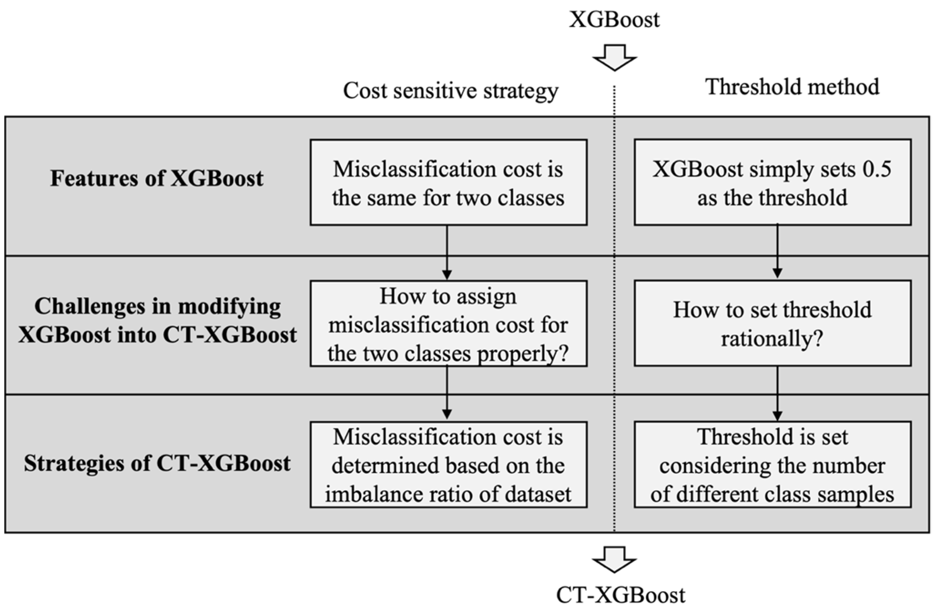
In this section, we present the novel CT-XGBoost prediction model with cost-sensitive and threshold methods. Figure 1 shows how XGBoost is modified into CT-XGBoost in this paper. In XGBoost, the misclassification costs for both classes are the same, and the threshold is simply set as 0.5. Thus, we improved XGBoost, turning it into CT-XGBoost, by solving two challenges: How to assign misclassification costs for the two classes properly. How do you set the threshold rationally? In this paper, two corresponding strategies (cost-sensitive strategy and threshold method) are adopted to overcome the challenges, misclassification cost is determined based on the imbalance ratio of the dataset, and a threshold is set considering the number of different classes samples. Then, XGBoost is modified into CT-XGBoost systematically.

In order to introduce CT-XGBoost logically, we first explain the theory of XGBoost and then illustrate how we modify XGBoost into CT-XGBoost. After that, the commonly used default prediction models are introduced, which are used to compare with our proposed model. Lastly, performance evaluation methods of the credit default prediction are explained.

3.1. XGBoost

XGBoost [19], the full name of which is extreme gradient boost, is a distributed and efficient implementation of gradient boost tree. It is an improved model based on the gradient boosting decision tree (GBDT), which belongs to the family of boosting methods. The chief idea of XGBoost is to incorporate a series of weak learners into a strong learning algorithm [2]. By adding new weak learners, the probability of making mistakes is reduced continuously, and the final output value is the sum of the results of many weak learners. To better understand the mechanism of XGBoost, the prediction function, objective function, and optimization process are introduced as follows.

Considering a dataset with n substances and m features, where $D=\left\{\left(x_i,y_i\right)\right|x_i\in R^m,y_i\in R$} and $x_i=\left\{x_{i1},x_{i2},\dots ,x_{im}|i=1,2,\dots ,n\right\}$. The basic idea of XGboost is to iteratively construct $t$ weak estimators to predict the output $y_i$ by the predictor $x_i$.

$$\begin{gathered} {\widehat{y}}_i^0=0 \\ {\widehat{y}}_i^1=f_1\left(x_i\right)={\widehat{y}}_i^0+f_1\left(x_i\right) \\ {\widehat{y}}_i^2=f_1\left(x_i\right)+f_2\left(x_i\right)={\widehat{y}}_i^1+f_2\left(x_i\right) \\ \dots \\ {\widehat{y}}_i^t={\displaystyle \sum }_{k=1}^t{f}_k\left(x_i\right)={\widehat{y}}_i^{t-1}+f_t\left(x_i\right) \end{gathered}$$

(1)

Each weak estimator$f_k\left(x_i\right),k=1,2,\dots t$ is generated from the iteration of the gradient boosting algorithm, and the output value ${\widehat{y}}_i^t$ is the summation of the output value of previous iteration ${\widehat{y}}_i^{t-1}$ and the present result$f_t\left(x_i\right)$. To learn the set of estimators, the objective function that needs to be minimized can be expressed as:

$$L^t\left(y, {\widehat{y}}^t\right)={\sum }_{i=1}^{n}l\left(y_i, {\widehat{y}}_i^t\right)+{\sum }_{k=1}^t\Omega \left(f_k\right),$$

(2)

where$l\left(y_i, {\widehat{y}}_i^t\right)$ is the loss function that measures the difference between the target value and the prediction value ${\widehat{y}}_i^t$. The second term is the regularization of the model, which is used to penalize the complexity of the entire model, and it can be calculated as follows:

$$\Omega \left(f_k\right)=\gamma T_k+\frac{1}{2}\lambda {\sum }_{j=1}^{T_k}{w}_{kj}^2,$$

(3)

Here, $T_k$ represents the number of leaf nodes in the $k-$th base tree estimator, and $\gamma$ is the penalty parameter for the number of leaf nodes. Meanwhile,$w_{kj}$ represents the weight of the $j-$th leaf node in the base tree estimator and $\lambda$ is the penalty parameter for the leaf node weight.

Up to now, we have a basic idea about the chief goal of XGBoost [19]. Next, we will introduce the process of how to optimize the objective. First, considering the training process is an additive consideration, as in Equation (1),$f_t$ is greedily added to minimize the objective, when predicting the output value ${\widehat{y}}^t$ at the t-th iteration.

$$L^t={\displaystyle \sum }_{i=1}^{n}l\left(y_i, {\widehat{y}}_i^{t-1}+f_t\left(x_i\right)\right)+\Omega \left(f_t\right)$$

(4)

Using the second gradient approximation of the Taylor explosion, Equation (4) can be expanded as follows.

$$L^t\cong {\displaystyle \sum }_{i=1}^n\left[l(y_i, {\widehat{y}}_i^{t-1})+g_i{f}_t\left(x_i\right)+\frac{1}{2}{h}_i{f}_t^2\left(x_i\right)\right]+\Omega \left(f_k\right)$$

(5)

where $g_i$ and $h_i$ indicate first and second gradient statistics. By removing the constant term $l(y_i, {\widehat{y}}_i^{t-1})$, we can obtain the simplified objective as follows.

$${\tilde{L}}^t\cong {\displaystyle \sum }_{i=1}^n\left[g_i{f}_t\left(x_i\right)+\frac{1}{2}{h}_i{f}_t^2\left(x_i\right)\right]+\Omega \left(f_k\right)$$

(6)

Define the set of samples of the j leaf node as $I_i=\left\{i|q\left(x_i\right)=j\right\}$ and then expand the regularization term.

$$\begin{gathered} {\tilde{L}}^t\cong {\displaystyle \sum }_{i=1}^n\left[g_i{f}_t\left(x_i\right)+\frac{1}{2}{h}_i{f}_t^2\left(x_i\right)\right]+\gamma T_t+\frac{1}{2}\lambda {\displaystyle \sum }_{j=1}^{T_t}{w}_{tj}^2 \\ ={\displaystyle \sum }_{j=1}^{T_t}\left[G_j{w}_{tj}+\frac{1}{2}\left(H_j+\lambda \right)w_{tj}^2\right]+\gamma T_t \end{gathered}$$

(7)

where $G_j={\sum }_{i\in I_j}{g}_i$ and $H_j={\sum }_{i\in I_j}{h}_i$. Then, the optimal weight $w_j^{*}$ of leaf$j$ can be computed by

$$w_j^{*}=-G_j{H}_j+\lambda$$

(8)

and we get the corresponding optimal objective value by substituting $-\frac{G_j}{H_j+\lambda }$ for $w_j^{* }$ in Equation (8).

$${\tilde{L}}^t\left(q\right)=-\frac{1}{2}{\displaystyle \sum }_{j=1}^{T_t}\frac{G_j^2}{H_j+\lambda }+\gamma T_t$$

(9)

where ${\tilde{L}}^t\left(q\right)$ is used as the assessment function to evaluate the quality of the tree structure $q\left(x\right)$. Specifically, the smaller the value of ${\tilde{L}}^t\left(q\right)$, the higher quality of the tree structure.

So far, the model with the T base estimator has been basically constructed and the prediction value of XGBoost is ${\widehat{y}}_i^t$, which can represent the default probability of the $i$-th corporate in this paper.

3.2. CT-XGBoost

XGBoost is a strong approach for various tasks. Nonetheless, the efficiency of the model can be limited due to the class-imbalance problem in the credit default data. Thus, it may be a good idea to modify XGBoost to adapt to the class imbalance of the credit default dataset. Assume the credit default dataset for the training model contains $N$ samples in total, where the number of credit default samples is $N_d$ and the number of non-default samples is $N_n$. In the real world, the number of default samples is hugely greater than the number of non-default samples, which causes the class-imbalance problem with the imbalance ratio defined as $\frac{N_n}{N_d}$. To solve the problem, we proposed a novel CT-XGBosot, which is modified from the XGBoost model.

Specifically, we modified the XGBoost in two aspects: (1) The cost-sensitive strategy is employed to assign more misclassification costs for default class samples relative to non-default class samples. During the calculation of the loss function, a novel parameter, called the penalty ratio in this paper, is added to control the ratio of misclassification costs for different classes. (2) We set a more reasonable threshold considering the class imbalance, which is used to classify the samples into two groups based on the predicting default probabilities. The corporates with default probabilities above the threshold are classified as the default group, and those with default probabilities below the threshold are classified as the non-default group. The modification will be explained in detail as follows.

3.2.1. Cost-Sensitive Strategy

In the process of default prediction model training, an important step is to calculate the objective function. Equation (2) is the objective function of XGBoost. In Equation (2), the first term ${\sum }_{i=1}^{n}l\left(y_i,{\widehat{y}}_i^t\right)$ is the loss function, which measures the disparity between the prediction results and the true results [23].

However, the importance of each sample to the loss function is the same. The misclassification costs of default class and non-default class samples are equal. Due to the class imbalance problem where the non-default samples are the majority, the contribution of non-default samples to the loss may be larger than that of default samples. The model may wrongly take the chief aim of correctly classifying the non-default samples. Thus, it is important to modify XGBoost by assigning more misclassification costs to default class samples in the training process.

In CT-XGBoost, to increase the misclassification cost of default class samples, we modify the loss function ${\sum }_{i=1}^{n}l\left(y_i,{\widehat{y}}_i^t\right)$ as follows.

$${\displaystyle \sum }_{i=1}^n[y_i\ast C_d\ast l(y_i,{\widehat{y}}_i^t)+\left(1-y_i\right)\ast C_n\ast l(y_i,{\widehat{y}}_i^t)]$$

(10)

where $C_d,C_n$ are the weights of misclassification costs for default and non-default class samples. Since the magnitudes of $C_d,C_n$ do not influence the training process, we define a new parameter $p$, called penalty ratio, which equals to $\frac{C_d}{C_n}$. In this paper, we set penalty ratio $p$ as the dataset imbalance ratio $\frac{N_n}{N_d}$. Then, the loss contributed by default samples will be larger than before.

3.2.2. Threshold Method

Considering the default prediction is essentially a binary classification, a threshold is crucial to be set to determine the predicted default probability should be divided into which category. Corporates with default probabilities higher than the threshold are regarded as default class, and those with default probabilities lower than the threshold are regarded as the non-default class.

However, most of the previous prediction methods simply set 0.5 as the threshold, which is not suitable for imbalanced data [42]. For instance, if the default probability generated by the prediction model is a uniform distribution of $\left[0,1\right]$ and the threshold is set as 0.5, half of the samples will be classified as a default class, which results in many non-default samples being misclassified. Thus, how to set a rational threshold is an important problem for default prediction.

In the CT-XGBoost model, we set a rational threshold which equals the $N_d$-th highest default probability in the training dataset. After the default probability of the testing dataset is predicted, corporates with default probabilities higher than the threshold are classified as default corporates, and those with default probabilities lower than the threshold are classified as non-default corporates.

3.3. Benchmark Prediction Models

For the performance evaluation of our proposed model, we compared its default predictive ability to those of other models widely used in the literature. Thus, we constructed a statistical method with logit regression, and intelligent techniques, including support vector machine and neural network. Moreover, ensemble models, random forest and XGBoost [42], were also constructed as benchmark models. The following content will simply introduce these benchmark models, except XGBoost, which has been explained in Section 3.1.

3.3.1. Logistic Regression

Logistic regression is one of the most popular models in credit default prediction due to its simplicity and interpretability [3]. Logistic regression overcomes the limitation of the linear regression model, which requires that the explained variables obey a normal distribution and be continuous. To design a failure prediction model, this method aims to estimate the probability of corporate failure based on the explanatory variables. The model can be expressed as follows:

$$P\left(Y=1|X\right)=\frac{e^{{\beta }_0+{\beta }_{1}X}}{1+e^{{\beta }_0+{\beta }_{1}X}}$$

(11)

where $X$ is the vector of explanatory variables, $Y$ is the indicator of corporate failure, ${\beta }_1$ is a vector of coefficients, and ${\beta }_0$ is a scale parameter. The parameters ${\beta }_0,{\beta }_1$ are estimated by the maximum likelihood method. With this method, we can forecast corporate failure by comparing the possibility to a threshold and further interpret the variables by the coefficients of each variable. To prevent overfitting, we apply $l_1$ and $l_2$ regularization.

3.3.2. Support Vector Machine

As a distribution-free and robust machine learning method, SVM has been commonly applied in the domain of credit default risk assessment [31]. In brief, SVM is a generalized linear model which constructs an optimal hyperplane as a decision boundary. The decision boundary ensures the accuracy of correct classification while maximizing the separation between the boundary and the closest samples. The samples nearest to the optimal hyperplane are called support vectors [3]. All other training samples are irrelevant for determining the optimal hyperplane. The optimized strategy of SVM is to address a convex quadratic programming problem. To separate samples with non-linear relationships, non-linear kernel functions are adopted to project input vectors into a high-dimensional vector space in which the samples become more separable [42]. To avoid overfitting, we adjust the penalty for misclassification.

3.3.3. Neural Network

Neural network, also called deep learning, is one of the most popular artificial intelligence techniques and has also been commonly used in the field of corporate failure prediction. This model operates analogously to human neural processing and consists of numerous neurons. When tacking the binary classification tasks, the neural network typically includes three layers of network: (1) the input layer consists of as many neurons as the dimensionality of input variables, (2) hidden layers consist of a given number of neurons that is set by user, and (3) the output layer consists of one neuron which is used to divide the input sample [5]. The neurons in a particular layer are linked to both the preceding and the following layer. For every single neuron, the corresponding value is calculated by the sum of its inputs with weights and a given non-linear function. During the training procedure, the weight parameters in a neural network are adjusted step by step by back-propagation to narrow the differences between outputs and true values [5]. When the epoch set beforehand arrives, the training process stops and the output value is divided into a specific category according to a threshold. For the overfitting problem, we employ the dropout method, which randomly switches off portions of the connection during the training process.

3.3.4. Random Forest

Random forest is a supervised machine learning technique that consists of multiple decision trees. It is a modification of the bagging ensemble learning approach, and the classification process is determined by the integration of the categories output by a series of individual trees. In this research, random forest built a number of decision tree classifiers that were trained step by step on bootstrap replicates of the credit default dataset through randomly selecting explanatory variables. According to the majority voting result from the decision trees, the model provides the classification of observations. Moreover, the model can identify the importance of each variable based on its information gain. Importantly, to obtain the generalization performance, we adopted the commonly used method in decision trees by controlling the number of trees in the random forest.

3.4. Performance Evaluation for Credit Default Prediction

To assess the out-of-sample performances of credit default prediction models, we adopted the split methods used by previous research [5]. We randomly divided the dataset into a training dataset and test dataset in an 80% to 20% ratio. Due to the class imbalance of the dataset in which non-default samples represent the majority group, we used a stratified sampling method for splitting to ensure the same population structure of training data and testing data.

Considering that credit default prediction is a binary classification problem, we can evaluate the out-of-sample performance via the metrics for classification models. One common metric is overall accuracy, defined as follows:

$$Overallaccuracy=\frac{TP+TN}{TP+FN+FP+TN}$$

(12)

where TP (true positive) is the number of default companies which are correctly classified as default; FN (false negative) is the number of default companies which are wrongly classified as non-default; TN (true negative) is the number of non-default companies which are correctly classified as non-default; and FP (false positive) is the number of non-default companies that are wrongly classified as default.

Given the class-imbalance problem for the credit default prediction, the prediction performances of the two classes needed to be evaluated separately. For this purpose, type I accuracy and type II accuracy were taken into account. Type I accuracy (or sensitivity) is defined as the proportion of default samples predicted by the model correctly, and type II accuracy (or specificity) is defined as the proportion of non-default samples correctly predicted by the model.

$$TypeIaccuracy=\frac{TP}{TP+FN}$$

(13)

$$TypeIIaccuracy=\frac{TN}{TN+FP}$$

(14)

Moreover, the area under the receiver operating characteristic curve (AUC) is a popular estimation of a classification model’s overall performance [5]. The ROC curve is a graph consisting of two-dimensionality, on which one axis is the true positive rate (sensitivity) and the other axis is the false positive rate (1-specificity). While changing the default probability threshold, the curve would plot each point representing the true positive rate and false positive rate. For the reason that AUC is a part of the unit square area, its value shall always range from 0 to 1.0 [37]. In addition, AUC should be more than 0.5 for the model to be realistic, and the closer it is to 1, the better the prediction performance of the default prediction model.

4. Empirical Results

4.1. Data

We used a database of bank-loan defaults of firms in the west region of China for 2017–2021. The database was sourced from a bank in Xinjiang province of China. The database consists of the loan information and the financial statements of firms that are the debtors of the bank. According to the Industrial classification for national economic activities in China (GB/T 4754), we selected the companies in the energy sector. A firm is defined as defaulting if it fails to pay the loan periodically. The remaining companies are defined as non-default. The number of default firms is 205, and the number of non-default firms is 33, making the imbalance ratio about 6.21.

In determining the variables used to assess credit default risk, the majority of academic studies use financial variables as predictors of the default prediction models [43,44]. For instance, representative work by Beaver [21] constructed 30 financial variables from the financial statement, and the results demonstrated that the financial variables could provide a superior ability to predict corporate default. Thus, in this paper, we construct a comprehensive list of financial variables, including all accounting items in the financial statements. The reason for the selection of all accounting items but not a portion of accounting items was to avoid eliminating potentially useful information after discarding the unselected variables.

4.2. Credit Default Prediction Performance

In this section, we present a comparative analysis between our proposed CT-XGBoost model and other commonly used models, including logistic regression, SVM, neural network, random forest, and XGBoost.

Table 1. Credit default prediction performance comparison analysis of different prediction models.

Models	Logistic Regression	SVM	Neural Network	Random Forest	XGBoost	CT-XGBoost
Overall accuracy (%)	94.34	93.05	94.17	94.17	94.54	89.58
Type I accuracy (%)	65.25	68.37	54.29	65.71	71.07	91.43
Type II accuracy (%)	96.36	98.24	98.03	98.53	99.02	89.27
AUC (%)	92.86	94.36	90.35	94.70	95.44	96.38

Note: The number in bold-face indicates the best performance for each metric.

summarizes the average prediction results of different models with ten times 5-fold cross-validation. Among conventional models, XGBoost showed superior performance with an AUC value of 95.44%, and its other evaluation results are also superior. Similarly, Zhang and Chen [10] found that, compared with logistic regression, SVM, random forest, and et al., XGBoost achieves better credit default prediction performance: 91.4% AUC. Moreover, Wang et al. [35] constructed the XGBoost model for default prediction and found that the prediction performance in terms of AUC was 88.07%. By comparison, the credit default prediction performance in our study is better than in previous studies. The main reason for the difference between the results of this study and previous studies is the different default datasets used. We focused on the credit default companies in the energy industry. Overall, these results demonstrate that the XGBoost model is an efficient algorithm for credit default prediction, and it is rational to select XGBoost as the model to be modified for its superior performance.

It is notable that the chief aim of credit default prediction is to accurately identify as many default samples as possible without misclassifying too many non-default samples. However, the prediction performance of XGBoost has not met our expectations, with the type I accuracy value of only 71.07%, whereas the type II accuracy value is 99.02%. The reason for this phenomenon is the class imbalance problem, which causes the prediction model to be overwhelmed by the majority of non-default samples. Thus, this study proposes a novel CT-XGBoost to solve the class imbalance problem.

First, comparing the type I, type II, and overall accuracy, we can see that the CT-XGBoost model is more rational than other conventional models. We can see that the type I accuracy value of CT-XGBoost is 91.43%, which is 20.36% higher than that of the representative XGBoost model. The result implies that our proposed model has a superior ability to identify default class samples. Second, while the type II and overall accuracy values of our proposed model are lower than those of other models, the accuracy values of sacrifice are 9.75% and 4.96%, respectively, which are lower than the benefit in type I accuracy. In addition, the main aim of credit default prediction is to accurately identify the default class samples. Finally, as for the AUC value, which can evaluate the comprehensive performance of the prediction model, we can notice that our proposed model is better than benchmark models. The average AUC value of CT-XGBoost was 96.38%, which is better than the AUC values of other default prediction models, which ranged from 90.35% to 95.44%. These results suggest that our proposed model, which modifies the XGBoost model with cost-sensitive and threshold methods, outperforms other benchmark models when dealing with the class-imbalance problem.

4.3. The Importance of Predictor

A practical default prediction model should have not only good accuracy, but also a clear, interpretable result. To make the model acceptable for users, transparency in the decision process is indispensable. For instance, according to the Equal Credit Opportunity Act of the U.S., the creditors are mandated to provide applicants, upon request, with specific reasons underlying credit denial decisions. In previous studies [35,36], some methods are proposed to identify the significant performance drivers of the XGBoost model in default prediction. In this study, we applied the “Feature Importance” function to estimate the importance of the financial features used in our proposed CT-XGBoost model.

Before introducing the “Feature Importance” function, the splitting mode of leaf nodes in CT-XGBoost needs to be explained. First, a portion of features is selected as a candidate set. Then, determine a split point of the leaf node in the tree by using a greedy algorithm and calculating the Gini score to determine the best splitting point. Define $I_L$ and $I_R$ as the sample sets of leaf nodes and right nodes after splitting. Assume $I=I_L+I_R$; then, the objective function value ${\tilde{L}}_{no-split}^t$ before splitting and the objective function value ${\tilde{L}}_{split}^t$ can be obtained as follows:

$${\tilde{L}}_{no-split}^t=-\frac{1}{2}\frac{{\left(G_L+G_R\right)}^2}{H_L+H_R+\lambda }+\gamma T_{no-split}$$

(15)

$${\tilde{L}}_{split}^t=-\frac{1}{2}\left[\frac{G_L^2}{H_L+\lambda }+\frac{G_R^2}{H_R+\lambda }\right]+\gamma T_{split}$$

(16)

where $G,H$ are the first derivatives and the second derivatives after splitting, and subscripts $L,R$ indicate the left and the right node. Then, loss Gain value for leaf nodes in the $t$-th tree can be calculated, and the node with the highest Gain value is determined as the splitting point.

$$Gain=\frac{1}{2}\left[\frac{G_L^2}{H_L+\lambda }+\frac{G_R^2}{H_R+\lambda }-\frac{{\left(G_L+G_R\right)}^2}{H_L+H_R+\lambda }\right]-\gamma$$

(17)

The Gain value can be used to estimate the importance of features, which measures the ability to classify the default and non-default samples. Considering that CT-XGBoost is a model where a number of trees should be simultaneously considered, we calculated the “Feature Importance” function for the $r$-th feature as follows:

$$Importanc{e}_r=\frac{{{\displaystyle \sum }}_{k=1}^{t}Gai{n}_r^k}{{{\displaystyle \sum }}_{r=1}^m\left({{\displaystyle \sum }}_{k=1}^{t}Gai{n}_r^k\right)}$$

(18)

$Gai{n}_r^k$ is the Gain value for the $r$-th feature in the $k$-th tree, $t$ is the number of trees, and $m$ is the number of features. So far, the “Feature Importance” function has been explained, and the importance of financial variables can be calculated with Equation (15).

Table 2. Feature importance of the top 20 important financial variables in the CT-XGBoost model.

Rank	Financial Features	Feature Importance
1	Other receivables	0.237242
2	Sales expense	0.080695
3	Long-term deferred	0.051185
4	Non-operating income	0.048665
5	Long-term equity investment	0.044733
6	Accounts receivable	0.038403
7	Taxes	0.034495
8	Prepaid accounts	0.034344
9	Liabilities and owners’ equity	0.034228
10	Capital reserves	0.032203
11	Cash flow generated from operating activities net amount	0.030894
12	Intangible assets	0.026951
13	Operating costs	0.025119
14	Inventories	0.024920
15	Construction work in process	0.023612
16	Net increase in cash and cash equivalents	0.020937
17	Cash flow generated from investing activities net amount	0.019130
18	Advance from customers	0.017562
19	Operating revenue	0.016754
20	Bill receivable	0.015882

represents the feature importance results of the top 20 most important financial variables, ranked based on the feature importance values from highest to lowest. Starting with the most important, the ten features that contribute to the CT-XGBoost model’s credit default prediction ability are: (1) other receivables, (2) sales expense, (3) long-term deferred, (4) non-operating income, (5) accounts receivable, (6) taxes, (7) prepaid accounts, (8) liabilities and owner’s equity, (9) capital reserves, and (10) cash flow generated from operating activities net amount. The higher the feature’s importance, the stronger ability of the financial variable to classify the default and non-default samples. The results may be of great worth for practitioners, as they can help explain why an applicant is classified as a credit default class.

4.4. The Influence of the Parameter Setting in CT-XGBoost

As mentioned in Section 3.2, our proposed CT-XGBoost model has modifications in the form of two algorithm-level methods: the cost-sensitive strategy and the threshold method. The parameter in the cost-sensitive strategy is the penalty ratio, which can assign different misclassification costs to different class samples, and the parameter in the threshold method is the threshold value, which can be used to classify the default probabilities into two classes. Considering that these two parameters can influence the performance of CT-XGBoost, we further analyzed how the credit default performance changes with different parameters and found the best parameter settings.

4.4.1. Parameter Setting for Cost-Sensitive Strategy

The chief aim of the cost-sensitive strategy in the CT-XGBoost model is to assign different misclassification costs to different class samples. The parameter for the cost-sensitive strategy is the penalty ratio $p$, which is the misclassification cost ratio between the default class and the non-default class. In Section 3.2.1, we set parameter $p$ as $\frac{N_n}{N_d}$, where $N_n,N_d$ are the numbers of non-default and default samples in the training dataset, respectively. The results in Section 4.2 demonstrate that a cost-sensitive strategy in CT-XGBoost is helpful for class imbalance credit default prediction. In this section, we investigate the influence of penalty ratio $p$ in the cost-sensitive strategy on the prediction performance of the CT-XGBoost model. 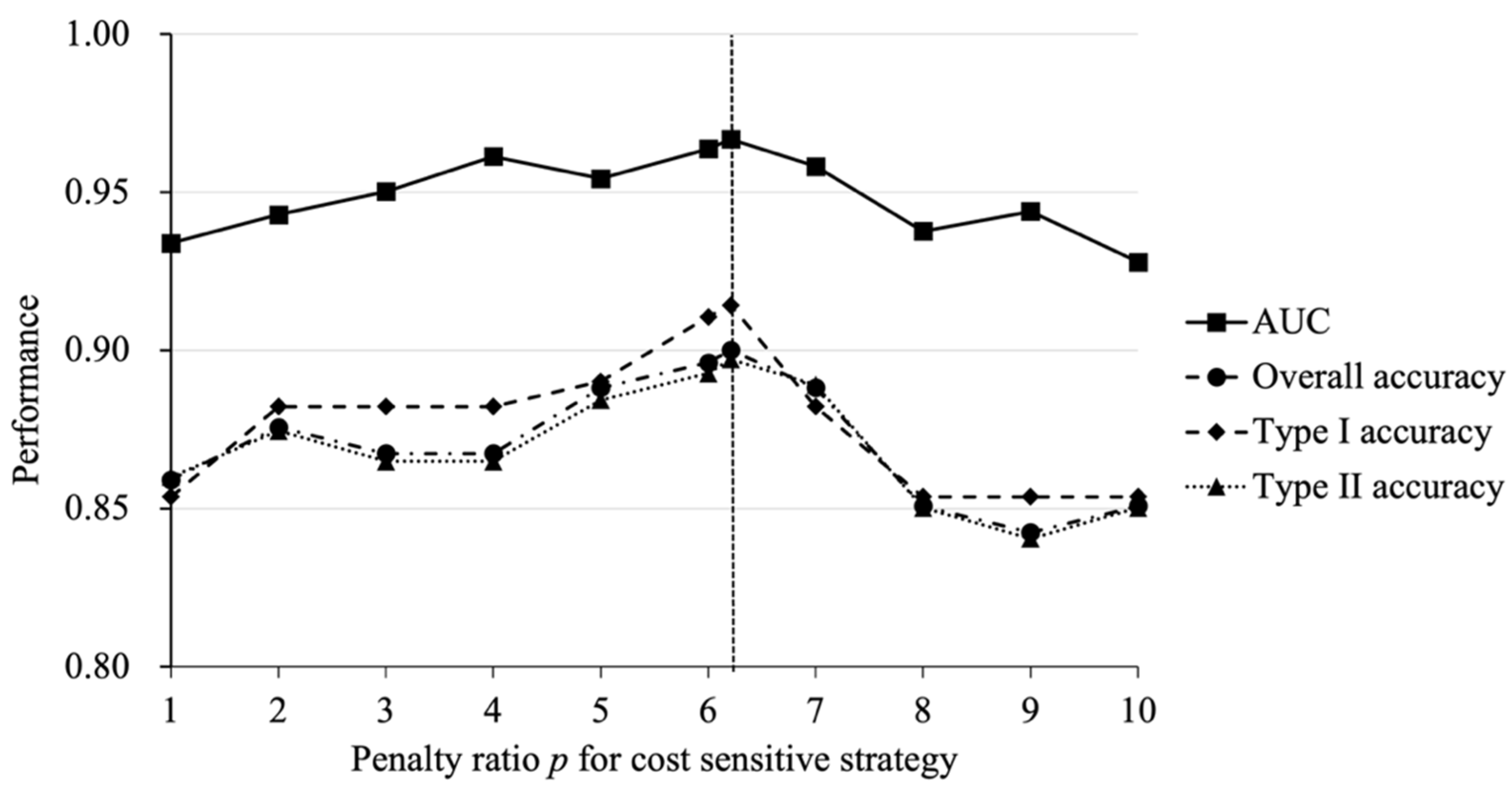We set the penalty ratio $p$ to range from 1 to 10 with increments of 1, and also 6.21 (the imbalance ratio of the dataset). The higher $p$ is, the more misclassification costs are assigned to the default class samples. For fixing the parameters of the threshold method to those in Section 3.3.2, the figure shows the results.

First, we can notice that there are fluctuations in the prediction performance at different values of penalty ratio $p$. As the value of $p$ increases from 1 to 10, the curves of the four performance metrics changes with similar trends, which are roughly upward and then downward. The results suggest that the default prediction performance can be better when more misclassification costs are assigned to default class samples; at the same time, high misclassification costs may not benefit the prediction model. This means that an appreciable penalty ratio $p$ is important for default prediction. As shown by the dotted line in Figure 2, the prediction performance of the CT-XGBoost model was best when the penalty ratio $p$ was set as 6.21, which is the imbalance ratio in the training dataset. Thus, it is crucial to consider the class distribution in the dataset when setting the penalty ratio $p$ for the cost-sensitive method.

4.4.2. Parameter Setting for Threshold Method

The role of threshold setting in CT-XGBoost is to classify samples with the predicting default probabilities into two groups. The sample is considered as default when the default probability is higher than the threshold, and non-default in reverse. As mentioned in Section 3.2.2, we set the threshold value as the default probability value of the $N_d$-th sample in the training dataset. In practice, the threshold determination is useful for controlling credit risk, and the creditors, such as banks, can control the number of debtors by adjusting the threshold for deciding whether to approve a loan. A higher threshold value means more applicants will be considered as non-default and approved for a loan. Meanwhile, the creditors will face higher credit risk. Therefore, investigating the influence of threshold setting on the default prediction performance is very important. In this studies, we varied the threshold value according to the predicting probabilities of samples in the training dataset. 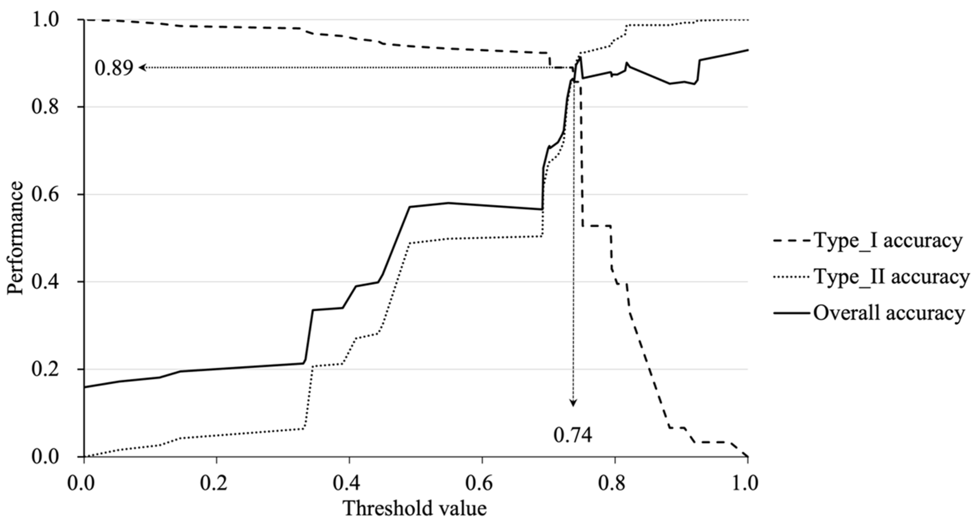For fixing the penalty ratio $p$ to the optimal value of 6.21, the results are presented in Figure 3.

We can see that as the threshold increases from 0 to 1, the curve of type I accuracy shows a downward trend, and the curves of type II and overall accuracy show similar upward trends. These results demonstrate that the prediction performance can be significantly influenced by threshold setting. When setting a lower threshold value, more potential credit defaults can be identified, but more true non-default cases can be mis-considered as default. In addition, the three curves in Figure 3 intersect when the threshold value is 0.74; default and non-default samples can be identified equally accurately. When the threshold value increases based on 0.74, the type I accuracy decreases rapidly, but the type II accuracy increases slightly. Thus, it is proper to set the threshold to around 0.74 in this case.

Moreover, the creditor can find the optimal threshold value based on its credit risk tolerance ability. When the creditor has weak credit risk tolerance ability, the threshold can be set low to obtain a high type I accuracy, which means the majority of potential default applicants are identified. However, we should notice that the type II accuracy can be low caused by a low threshold, which means a large number of risk-free clients would be turned away. To avoid losing huge benefits, assuming that the creditor can tolerate about 10% of default cases, the proper type II accuracy threshold is about 0.74, which means that about 89% of potential credit default applicants can be accurately identified. At the same time, the type II accuracy can be limited to 89%, which means that the creditor would only lose about 11% of free-risk clients.

5. Conclusions

In order to accurately predict the credit defaulting of energy corporates, the class-imbalance problem in the default dataset cannot be ignored. To tackle the problem, this paper proposed a novel and efficient default prediction model, CT-XGBoost, which was modified from the strong classification model XGBoost with the cost-sensitive strategy and threshold method. In the empirical analysis, we constructed a corporate credit default dataset from a commercial bank in China, which suffers from the class-imbalance problem. In order to evaluate the performance of our proposed CT-XGBoost, we selected five commonly used credit default prediction models as benchmark models, including logistic regression, SVM, neural network, random forest, and XGBoost. The empirical results demonstrate that our proposed CT-XGBoost outperforms the benchmark models. Therefore, the novel model CT-XGBoost can be helpful to solve the class-imbalance problem and assess the credit risk of energy companies efficiently.

We further analyzed the feature importance of the input financial variables, in order to identify the significant drivers which contribute to identifying the corporate defaults in the energy industry. The results show the top 10 most important features are: (1) other receivables, (2) sales expense, (3) long-term deferred, (4) non-operating income, (5) accounts receivable, (6) taxes, (7) prepaid accounts, (8) liabilities and owner’s equity, (9) capital reserves, and (10) cash flow generated from operating activities’ net amount. In practice, these financial variables in the company’s financial statements might be the key information for creditors to estimate the credit risk in the energy industry.

Moreover, we conducted sensitivity analysis to investigate how the different parameter settings in CT-XGBoost influence the prediction performance. The results show that the parameter in the cost-sensitive strategy, which represents the attention focused on the minority default companies, should be determined according to the actual ratio between the number of credit default and non-default companies. In addition, as the threshold value in the threshold method is set lower, type I accuracy decreases and type II accuracy increases. In practice, the threshold value represents the percentage of loan applications approved by creditors. According to their risk tolerance, the creditors can find the optimal threshold, which not only can control real losses caused by credit default but also the opportunity cost of rejecting too many loan applications.

In general, the novel model proposed in this study can efficiently estimate the credit risk of bank loans for energy companies, which is helpful for creditors who are making decisions. According to the results, this study proposes some recommendations: (1) As the crucial industry for economic development, energy companies should make the most of loan funds and avoid credit risk arising from cash flow problems. Meanwhile, energy companies should disclose more transparent information in timely manner, to help investors comprehensively understand the company’s operation and accurately assess the company’s credit risk. (2) In the credit loan market, the credit rating institutions should improve the credit rating system, which not only can efficiently assess the credit default probability but also can provide explainable reasons to ensure the reliability of the system. (3) The government and regulators should establish sound laws and regulations to promote a healthy development environment for the energy industry, including policy-based financial support, financial subsidies, fair credit law, etc.

Nonetheless, our research has several limitations which could promote future research. First, the class-imbalanced problem not only exists for credit default but also for financial fraud, as the fraudsters make up a minority of whole samples. Thus, it would be interesting to investigate whether our proposed model can help solve the class-imbalance problem in the default identification task. Second, in this paper, the information used to predict credit default is the financial variables of corporates, which is in a structured form. Future research can extend the horizons to investigate the default predicting ability of other unstructured information, such as news reports and meeting audio.