Abstract
This paper is concerned with designing a dynamical synchronization (via a robust cooperative control) of an electromechanical system network (EMSN), consisting of nonidentical brushed DC motors, where only the motors’ angular velocity measurements are available. The challenge of the proposed approach is that the actuation provided by the motor needs to handle external disturbances to achieve the velocity tracking task and handle the interaction between both motors cooperatively to share the load and the disturbance rejection. The control’s basis involves differential flatness and an active disturbance rejection control (ADRC) framework augmented using ideas from the graph theory analysis and multi-agent networks. Experimental results verify the theoretical developments and show the effectiveness of the proposed control strategy despite unexpectedly changing load disturbance and parameters uncertainties. The proposed algorithm is suitable for embedded use due to its simplicity. It can be applied to a broad spectrum of mechatronic systems where dual-motor drive arrangements are necessary.
1. Introduction
Mechanical systems with synchronization functionalities have been used for many complex applications that cannot be carried out by a single machine and/or individual mechanisms. Synchronization is a common phenomenon in nature [1] and it is necessary for engineering systems that collaborate to perform complex tasks, e.g., unmanned air vehicles, multi-robots, and sensor networks [2,3,4]. In particular, angular velocity synchronization and load-sharing in rotating mechanics systems for different applications have been topics of interest for motion control applications [5,6]. In this context, when the amount of torque applied to the load is prescribed and carried out by each drive and motor set, one speaks about load-sharing. As a consequence, cooperative control algorithms have to be developed to synchronize the speed and the torque of the participating motors robustly, to accomplish the different requirements to operate. Cooperation is a type of synchronization requiring all participants to interact to share information and cooperate toward achieving the goal [7,8]. The authors in [9] presented a control system that employs clock pulses to regulate and synchronize DC motors working at high velocities. The authors in [9] presented a control system to synchronize DC motors via clock pulses. This approach has unique features, such as precision and availability to restore equality in phases despite disturbances affecting the DC motor shafts. In [10,11], the problem of the load-sharing torque was studied for two DC motors with elastic shafts. In this work, the two engines provide the same torque to the entire load, provided that the motors have the same characteristics. Nevertheless, if the engines are not equal, they provide (only partially) a quantity of torque proportional to the nominal drive capacity. In [12], the authors described how two induction motors (IMs) provide the electric traction to a gantry crane, where a voltage/frequency control strategy allows distributing torque equally between the two induction motors to move the wheels of the crane subjected to slippages. Regardless, those above works do not explicitly present a cooperative control law that manages (at the same time) angular velocity tracking and load sharing.
For mechanical systems (second-order systems), high-gain control (also called proportional control) and proportional integral derivative (PID) control is an adequate solution because it is easy to implement for real-time applications [13]. Nevertheless, it is common knowledge that proportional control cannot completely remove the consequences of disturbances. Nonetheless, when a proportional integral derivative is employed, the integral term might efficiently reject the constant disturbance, although its performance is modest when time-varying disturbances are presented. In addition, the derivative mode of the PID is often removed due to the noise sensitivity [14]. Model reference adaptive control and adaptive control (AC) approaches are considerably efficient when the model parameters are uncertain [15]. This approach was recently applied in [16] to load sharing of two DC motors, which are identical in speed–torque characteristics. Nevertheless, under the presence of external disturbances, e.g., load torque, AC methods are limited since critical parameters are difficult to estimate in real-time [17]. In [18], an adaptive robust H-infinity control scheme is proposed to achieve both the load tracking and multi-motor synchronization of multi-motor servomechanism.
To suppress the influences of parameter uncertainties and external disturbances, the sliding model control (SMC) has shown satisfactory capabilities [19]. In [20], an SMC-based for the multi-motor is proposed. The authors in [21] propose an adaptive global sliding mode algorithm (AGSMC) to control a vibration system collaboratively. Nevertheless, it is common knowledge that discontinuous switching of the controller can be a source of high-frequency vibrations in mechanical and electromechanical systems [22,23], which is objectionable for servomechanisms. Lyapunov-based approaches have also been used for the design of synchronization controllers. In particular, in [24], a synchronization control technique for cable-driven parallel robots is presented.
Within the approaches, as mentioned earlier, the authors solved the load-sharing problem, mainly via well-designed and elegant feedback approaches that are robust towards the disturbance originated from the load. However, none of the reported works propose estimating the disturbance to cancel it later through a convenient electric current distribution in each electrical machine.
In the context of disturbance estimation and rejection, since the seminal work by Han [14], active disturbance rejection control (ADRC) has become central to designing control algorithms that allow online estimating disturbances caused by unknown system dynamics and exogenous disturbances. The “total disturbance” is estimated by the extended state observer (ESO) [25,26,27], the so-called disturbance-observer [28], and then “rejected”by combination of feedback and feed-forward terms [29].
The ADRC approach has been applied in many domains of control engineering, for instance: power filter design [30], energy storage [31], power plants [32], DC converters [33], electric machines and servomechanisms [34,35,36], or even renewable energy, together with cooperative control [37]. In recent years, due to the popularity of electric vehicles (EVs), ADRC has been applied to solve the problem of angular velocity synchronization between electric engines [38], where permanent magnet synchronous motors are used [39]. Nevertheless, the mentioned approaches do not consider a cooperative strategy. Moreover, the design is an observer sliding-mode-based. Very recently, an ADRC strategy [40] and an ADRC together with SMC [41] have been proposed for the synchronization control of parallel conveyors. However, as mentioned earlier, the load and external disturbances are not necessarily estimated with these approaches, which are required in our approach to conveniently distribute the electric current in each electrical machine.
Contributions
This work presents a cooperative active disturbance rejection control to share the load and synchronize the angular velocity of two non-identical brushed DC motors (see Figure 1). The considered model allows a network topology, i.e., we describe and interpret the system as an electromechanical system network (EMSN) affected by an unknown load torque, the flow of energy between each subsystem, and modeling uncertainties. The control design founded on differential flatness and an ADRC framework is boosted with the graph theory analysis and the multi-agent network approach. The present work is the follow-up to [42]. However, only the principle control design was presented in the latter work without giving a network topology interpretation and closed-loop performance analysis. Given the above literature, our contributions can be summarized as follows:
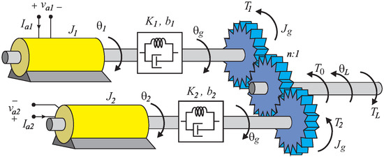
Figure 1.
Servomechanism driven cooperatively.
- We propose a novel robust cooperative control of an EMSN constituted of nonidentical brushed DC motors where only the motors’ angular velocity measurements are available.
- The key idea behind the proposed approach is that the actuation provided by the motor needs to handle the total disturbance associated with unknown parameters, unknown dynamics, or an external torque load to achieve the velocity tracking task. It also needs to handle the interaction between both motors cooperatively to share the load and the disturbance rejection.
- The information exchange in the cooperative control utilizes the physical communication network and digital communication between controller modules to achieve torque sharing using an agreement-like algorithm in the ADRC.
- We proved the input-to-state stability (ISS) properties of the closed-loop system.
- We scrutinized the closed-loop system’s effectiveness and advantages through real-time experiments in a controlled and instrumented set-up.
- A rigorous assessment of the robustness and tracking performance towards unexpectedly changing the load disturbance and parameter uncertainties was carried out.
- The proposed algorithm is suitable for embedded use due to its simplicity. It can be applied to a broad spectrum of mechatronic systems where dual-motor drive arrangements are necessary.
The remainder of the article is structured as follows. The preliminary theoretical aspects are introduced in Section 2. The system’s dynamic model and differential parameterization are presented in Section [43]. The cooperative ADRC design and the main results are introduced in Section 4. The efficacy of the control strategy is demonstrated experimentally in Section 5. Section 6 delivers the conclusions. Appendix A presents in detail the closed-loop stability analysis.
2. Preliminaries
2.1. Differential Flatness
Flatness (or differential flatness) is a property that generalizes the concept of linear controllability to the case of nonlinear systems. In the linear time-invariant and time-varying cases, it entirely coincides with the controllability concept. Flatness trivializes the system structure, under state transformation and partial feedback, to that of a pure integration system [44].
2.2. Input-to-State Stability (ISS)
In the following, denotes the Euclidean norm for vectors and the induced two-norm for matrices, respectively. A dynamical system, with state x and input w satisfies the input-to-state stability (ISS) property if there exists a class function and a class function such that for all . For a signal w, denotes the -norm: sup . For linear systems, ISS is equivalent to the global asymptotic stability of the unforced system [45].
Theorem 1
([45]). The following properties are equivalent for any system:
- It is ISS.
- It admits an ISS-Lyapunov function.
- It is robustly stable.
3. System’s Mathematical Model
From Figure 1, using Kirchhoff’s laws and the principle of angular momentum, the following dynamic model is obtained:
the involved symbols assigned to the variables and parameters are described in Table 1 where the subscript indicates the corresponding brushed DC motor.

Table 1.
Definition of symbols used in (1).
One aim is to represent the system as an electromechanical system network (EMSN), such as suggested in Figure 2.
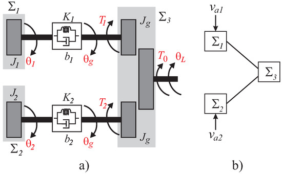
Figure 2.
(a) Electromechanical system network (EMSN) and (b) its interconnection topology.
Remark 1.
Let us consider only the mechanical part of the system and , together with . Furthermore, let us define , and with . The dynamics of these mechanical subsystems can be written in matrix form, as follows:
which has the form of a time-invariant linear system:
Note that represents the Laplacian matrix of the EMSN, which is symmetric and positive semi-definite, i.e., . Moreover, note that the row of sums of is zero. From graph theory, [7,8,46], it is known that the zero-input response of (12) decays to zero exponentially fast, whereas the zero-state response converges to a consensus (synchronization). That is, when . This implies that after a sufficiently long time, , which implies
Differential Flatness-Based Parameterization for the Servomechanism
To design the collaborative and decentralized control strategy, one considers the subsystems (8) and (9). As it was done previously, let us define , and with . Thus, (8) and (9) can be written as follows:
with .
On the other hand, it is well known that the Flat output of the DC motor system is the angular speed [43,44]. Therefore, the differential parameterization of all system variables, and the control vector , in terms of , and their time derivatives become:
with and where and represent the amount of endogenous and exogenous disturbances, respectively. Furthermore, is state-dependent and is (in general) unknown. However, both are considered to be functions of the time and are assumed to be uniformly absolutely bounded.
Remark 2.
The boundedness of comes from (12), which can be written as
with and . Since J is a diagonal matrix, represents the Laplacian matrix of the EMSN. As a consequence, the vector of one is an eigenvector corresponding to the eigenvalue [8]. Eigenvalues can be listed in increasing order, . Then, the solution of (18) for can be written as
by using the bound [47]
an upper bound on the norm of the trajectories of (18) is established as
The bound shows that the zero-input response decays to zero exponentially fast, whereas the zero-state response is bounded by every bounded input. Since components of the correspond to a linear combination of the armature current, stiffness torque, and load torque, which are bounded, then one always has a bounded input. Consequently, is always bounded. Since and are chosen to be the flat outputs, then with is, by definition, bounded, which corresponds with our assumption.
Let be the total disturbance with . Then, the differential parameterization (17) can be written as follows
Again, in the case that with are measured, and the system’s parameters are well known, this differential parameterization suggests the following collaborative and decentralized speed tracking controller with load-sharing
with
where represents the reference (desired) angular velocity for each motor ( being the desired angular velocity of the load shaft) and with and for and otherwise, represents the torque that has to develop each motor, such that the desired velocity is achieved. Consequently, the term represents the torque’s discrepancy between the motors. Let us define the speed tracking errors as: , , . Thus, the closed-loop system can be written as follows
If are chosen, such that the left-size of (23) is a Hurwitz polynomial, then, given some initial conditions, , when if and only if
Note that (24) represents the load-sharing condition, i.e., it represents the agreement protocol between the subsystems and to drive subsystem . Hence, according to Remark 1, the speed-tracking and load-sharing objectives are achieved.
4. Decentralized Active Disturbance Rejection Controller Design
Let us define and , then (20) can be written as follows
Before developing the active disturbance rejection controller, we assume the following:
- (a)
- Only the flat outputs are measured, for .
- (b)
- The nominal values of the set are known for .
- (c)
- The control inputs are available, for .
- (d)
- The disturbances functions () are uniformly absolutely bounded, i.e., for .
- (e)
- The disturbance estimation will be denoted by for .
- (f)
- The estimated variables of the flat outputs, and their successive derivatives, will be denoted by and , which correspond to the estimated and , respectively, and for .
ESO Design for the Decentralized ADR Controller
It follows that the estimation of the total disturbance is given by (see Proposition A1 and Remark A1)
The set of coefficients , , , are constant values, which are chosen with the help of a desired closed-loop Hurwitz polynomial of the fourth-order for the linear dominating dynamics of the injected estimation error dynamics.
Remark 3.(Estimation of the developed torque in each motor): From (17), the total disturbance is given by
Let us assume constant parameters, and . Hence, at a steady-state, the total disturbance becomes
Let and be the estimations of and respectively, which are obtained through (ESO) (26). Consequently, the developed torque by the motor i, such that the steady-state is achieved, is estimated as follows
Equation (30) is obtained assuming a steady-state. However, through many experiments, it has been corroborated that this assumption could be removed, and then we can use instead of .
Now, we are ready to announce our main result. The idea is to adapt the estimated values obtained from the observer (26) in the tracking controller. Thus, one has the following collaborative and decentralized speed tracking controller, ADRC-based with load-sharing capabilities:
with
where
for . The set of coefficients , are positive values, which are chosen with the help of a desired closed-loop Hurwitz polynomial of the second-order.
The interconnection topology of the overall system using the control law (31)–(33) is depicted in Figure 3, where the energy flow and information flow are represented using solid edges and dotted edges, respectively. In the experimental tests, we will demonstrate the importance of the digital torque coupling. The closed-loop system, depicting each subsystem, is shown as a block diagram in Figure 4.
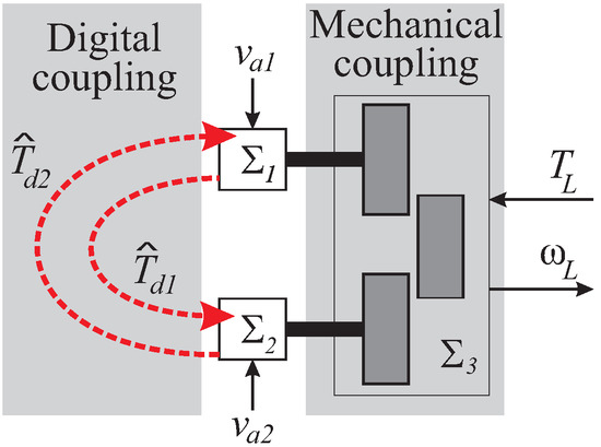
Figure 3.
Interconnection topology of the EMSN depicting energy flow (solid edges) and information flow (dotted edges).
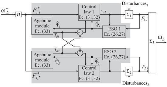
Figure 4.
General block diagram of the proposed control scheme.
Remark 4.
The proposed scheme for more than two motors can be applied in the framework of multi-agent systems. The digital torque coupling for the load-sharing could be implemented via a communication topology using undirected and connected graphs. Then, cooperative strategies, such as the leader-following consensus, could be used [48,49].
5. Experimental Results
A general schema and the experimental setup are depicted in Figure 5 and Figure 6, respectively. The setup comprises two DC power supplies, two full bridges, and two brushed DC motors coupled using two gearboxes to a common stiff shaft. Furthermore, the computational board is based on the TMS320F28335.
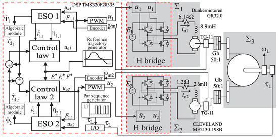
Figure 5.
Experimental setup scheme.
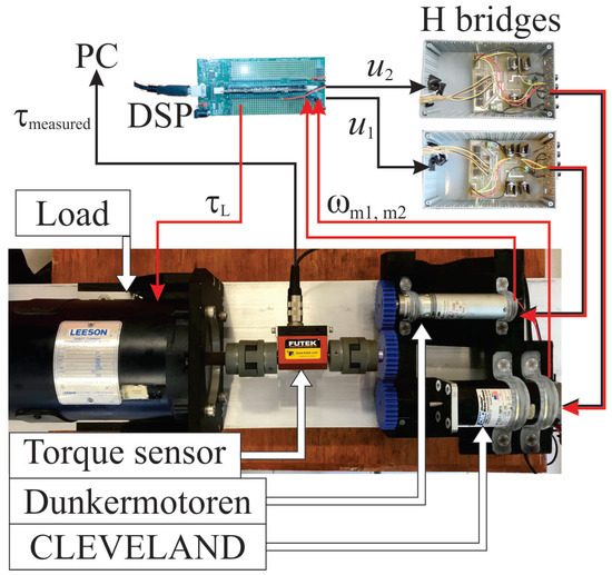
Figure 6.
Servomechanism drives by two brushed DC motors.
Each motor has a gearbox (PLG 32) with 50:1 [50], and a relation of the nominal output torque of 150 Ncm. The dynamic load torque applied to the servomechanism system (exogenous disturbance) is carried out using a DC motor and the torque load is measured through a rotary torque sensor (TRS605) [51]. For the servomechanism, the first DC motor is a Dunkermotoren GR42x25. This motor has a tachogenerator to measure the angular velocity (TG–11). Table II shows a summary of the electrical parameters for this motor. The second DC motor is a Cleveland ME2130–198B. This motor has an incremental encoder of 1000 lines/rev. Table III shows a summary of its electrical parameters. The Servomechanism’s parameters are given by kgm, Nm. Note that the DC motor parameters and are assumed to be equivalent [52].
The control algorithm is coded on a TMS320F28335 DSP board. The internal clock frequency in the processor is set to 150 MHz and the sampling frequency is adjusted to 1 MHz. Two incremental encoder modules, two PWM signal generators, and the digital output are required. Figure 5 depicts the involved elements and these are described below.
The flat output is measured by the A/D converter, and is measured by a dual-channel incremental encoder with a quadrature. The control inputs and adjust the duty cycle of the respective PWM module, which are set to a frequency of 10 kHz. The disturbance signal is driven via a digital output port of the DSP board, which allows enabling/disabling the applied disturbance load torque in the common stiff shaft.
The control-observer strategy is implemented for each motor. Each one has two modules, which are described below. In the module, the effects of the interaction and the load torque perturbations are estimated (, , ). The is implemented via a discretization using the implicit Euler method. The gains , , , are chosen in such a way that the eigenvalues are: , , for the 1 and , , for the 2. The gain is for both subsystems.
For the feedback term (32), the gains are chosen in such a way that the closed-loop eigenvalues are , , , .
In the module, we program the reference signal for the flat output , which is specified as follows:
with being an 8th-order Bézier polynomial given by
and
Figure 7a,b show the angular reference velocity , the angular velocity response to each DC motor, and the angular speed response corresponding to the common stiff shaft. One can see that the trajectory tracking task and angular velocity synchronization for the two DC motors are achieved approximately in 0.2 s, despite an applied external load torque, i.e., . The tracking velocity error (induced by unknown disturbances and the applied load torque) is shown in Figure 8, whose amplitude remains bounded. Each motor’s tracking velocity error bound is around 15 rad/s, representing of the maximum desired velocity.
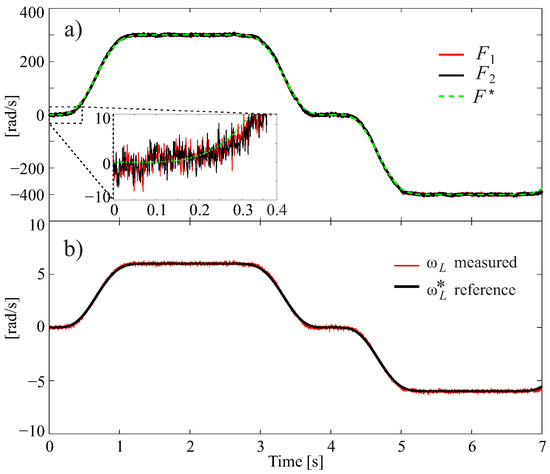
Figure 7.
Angular speed tracking responses: (a) in each subsystem M1 and M2, and (b) in the common stiff shaft.
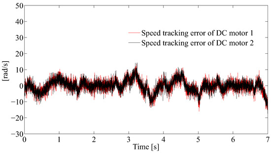
Figure 8.
Angular speed tracking error responses.
During experimentation, disturbances are applied to the common stiff shaft, whether the angular velocity reference is constant or time-varying. The applied load torque magnitude was around 4 Nm (see Figure 9a) to induce disturbances in the motors’ shaft, but without putting the system at risk.
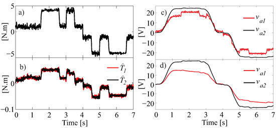
Figure 9.
(a) Load torque applied on the common stiff shaft, (b) internal developed torque on each brushed DC motor, input voltage response (c) with and (d) without digital torque coupling.
The challenges and contributions of the proposed approach are that the actuation provided by the motors not only needs to handle disturbances associated with unknown parameters, unknown dynamics, or the external torque load, but it also needs to handle the interaction between both motors cooperatively to share the disturbance rejection. For that, in each subsystem, the extended state observer (ESO) estimates the so-called total disturbance , which is required for the control law (31) to cancel it. In turn, allows estimating the disturbance torque with respect to the motor’s shaft, which is afterward used in the cooperative control law (32). Note that a key in the proposed control is the agreement term , which handles the interaction between both motors cooperatively to share the load and reject the disturbances collaboratively.
Figure 9a shows the load torque applied to the primary shaft system, while Figure 9b shows the motor’s developed torque to reject the disturbance. Here, we realize that the load torque distribution between the two DC motors is equitable. Thus the cooperative controller achieves its objective. On the other hand, Figure 9c,d show the input voltage response of each DC motor with and without digital torque coupling, respectively. One can see that the supply voltage is not similar because the DC motors have different characteristics (see Table 2 and Table 3). However, the supply voltage difference is more significant when digital torque coupling is not considered (see Figure 9d).
Table 2.
Data GR 42 × 25 DCM1.
Table 3.
Data ME2130-198B DCM2.
To demonstrate the advantages of the proposed control strategy, we conducted the same test with and without the agreement term, in the control law (31) and (32), seen as digital coupling. The comparison is shown in Figure 10. The evolution of the motor’s armature current is depicted for clearness instead of the torques. Figure 10a shows the performance of the proposed collaborative control. The difference in the armature currents is because the motors have different nominal parameters (see Table 2 and Table 3). Nevertheless, the developed torque is the same in each motor, as shown in Figure 9b.
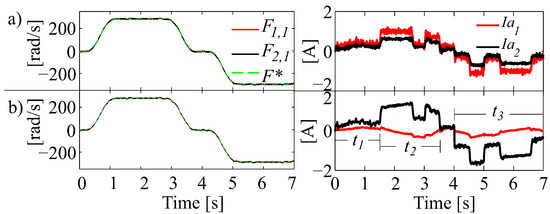
Figure 10.
Angular velocity response and its corresponding armature current responses: (a) with digital torque coupling and (b) without digital torque coupling.
On the other hand, Figure 10b shows the performance without the coupling mentioned earlier. Trajectory tracking is achieved in this case, and velocity synchronization is performed due to the gears’ mechanical system network. However, the load is not shared to reject the disturbance. This last can be corroborated through the evolution of the armature current. Note that system practically does not provide the current (torque) in the interval . Furthermore, during , works as a generator due to the external disturbance, and tracks the reference and annihilates the disturbance. Finally, during , provides a lesser amount of the current and the job is done by .
Robustness Evaluation against Parameter Uncertainties
To test the performance of the system under dynamic model parameter variations, an angular output speed reference rad/s was established. Moreover, the load torque profile shown in Figure 11 was applied. The tests consisted of the variation of parameters , , and , in the code of the proposed control scheme. We chose the parameters of the Cleveland CD motor () to achieve this task. Then, parameters , , and were scaled by the factor , which took values in the closed interval , i.e., .
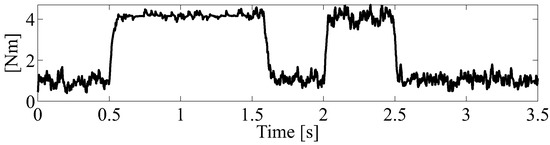
Figure 11.
Load torque applied in the dynamic model parameter variation tests.
Figure 12 and Figure 13 showed the response of the angular velocity error, , and the torque difference between the two CD motors, , respectively. These signals were obtained under motor 2 parametric variations: (Figure 12a,b), (Figure 12c,d), and (Figure 13a,b).
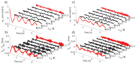
Figure 12.
Variation of : (a) , (b) ; variation of : (c) , (d) .
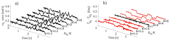
Figure 13.
Variation of : (a) , (b) .
Figure 12 demonstrates that the performance of the proposed control scheme worsens when the nominal values of and are scaled by a factor of and 7.7 (red signals). In other words, these nominal parameters can be scaled by without significantly decreasing the performance of the proposed control scheme. The system tolerates a relatively large variation of parameters and , maintaining the equitable cooperation of the load torque by the two motors. Note that these parameters are not necessary to obtain (Equation (33)).
On the other hand, the variation of affects the cooperation of the load torque between both motors as shown in Figure 13b. Therefore, by changing the value of this parameter, it is possible to adjust the percentage of the motor torque cooperation. Finally, it is worth noting that the variation of allows trajectory tracking, but one of the motors could stop working and could act as a current generator. Therefore, we need to know this parameter for the proposed control scheme. Fortunately, this parameter can be identified experimentally, relatively easily.
6. Conclusions
The proposed cooperative control strategy allows controlling the angular velocity of a servomechanism driven by two brushed DC motors while enabling it to carry out load-sharing. This dissection reveals that the observer is robustly stable, i.e., it satisfies the input-to-state stability (ISS) property, in the case that the total disturbance is considered as an input and the estimation error of the state. Furthermore, the speed-tracking control, together with an agreement-like algorithm in the ADRC, allows an equitable load-sharing, and it is shown to also be ISS. From a practical point of view, the experimental results confirm the hypothesis; the control strategy rejects the disturbances generated by the load torque applied to the primary shaft of the servomechanism under sudden load changes and synchronizes the angular speed of both DC motors. A key theoretical experimental result is that the cooperative control algorithm distributes the electric current conveniently in each electrical machine, even when these DC motors have different load capacities. Extensive experimental tests were performed to evaluate the robustness and performance against the uncertainty of some model parameters. This analysis reveals that the system tolerates a relatively large variation of inductance and inertial parameters, but it is sensible to the change in the torque constant . Fortunately, this parameter can be identified relatively easily.
Thanks to the electromechanical system network (EMSN) description used in the present work, the applicability to more than two motors is possible. Furthermore, we suspect that it is possible to adjust the percentage of motor torque cooperation by appropriately modifying the agreement term. Due to its simplicity and robustness, the proposed method can be used in a broad spectrum of applications where mechatronic servo systems are necessary.
Author Contributions
Conceptualization, J.L.-F. and J.F.G.-C.; methodology, W.F.G.-S. and J.F.G.-C.; software, A.H.-M. and V.R.G.-D.; validation, A.H.-M., G.M.A. and G.A.M.-H.; formal analysis, J.F.G.-C. and J.L.-F.; investigation, W.F.G.-S.; resources, G.M.A.; data curation, G.A.M.-H.; writing—original draft preparation, J.L.-F., W.F.G.-S. and J.F.G.-C.; writing—review and editing, J.F.G.-C. and V.R.G.-D.; visualization, A.H.-M.; supervision, J.L.-F.; project administration, J.F.G.-C.; funding acquisition, G.M.A. and G.A.M.-H. All authors have read and agreed to the published version of the manuscript.
Funding
This research was partially funded by VIEP-BUAP grant number 100305333-VIEP2021.
Institutional Review Board Statement
Not applicable.
Informed Consent Statement
Not applicable.
Data Availability Statement
Not applicable.
Conflicts of Interest
The authors declare no conflict of interest.
Appendix A. Closed–Loop Stability Analysis
Proposition A1.
Let be the estimation error and consider the extended state observer (26) and the servomechanism with two DC motors coupled through two cogwheels to a stiff shaft system (8)–(10). Then, the estimation error dynamics satisfy the ISO property (input to output stability) [45], i.e., the error dynamics state converges to a sphere centered at the origin of the estimation error phase space with the radius
where depends on the parameter design , . Moreover, the error dynamics presents asymptotic stability to for .
Proof.
Let the estimation error be defined as , then
The estimation error obeys the linear differential equations given by (A4), which can be written as the following LTI system in its space-state realization
where
The estimation error trajectories with initial condition and input perturbation are given by
If , are chosen, such that is Hurwitz, then one has the following bound [53]
where is the maximum eigenvalue of with . Now, it then follows that
As a consequence, when , converges exponentially to a sphere with radius □
Remark A1.
From (A2), it follows
according to Proposition (A1), , and converge to a small bounding sphere in the estimation error phase space. Then, tracks, arbitrarily close, the unknown total disturbance , the modulo motor parameters. It follows that,
Let be defined by
then,
which means that the error between the total disturbance and the estimated one evolves in a very small bounded sphere.
Remark A2.
Note that the estimated torque remains bound since all of the involved functions used to obtain it are bound. This boundedness becomes (33) and the results mentioned above; that is
since is assumed bounded, is bounded (see Remark 2) and and converge to a small bounding sphere in the estimation error phase space (see Proposition A1) then is bounded; that is, for .
Proposition A2.
The servomechanism (8)–(10) represented, employing its differential parameterization (20) with the control (31)–(33) is ISS if the position tracking error is considered the state and the input, where
with , such that sup. That is, converges exponentially to a sphere centered at the origin of the tracking error phase space with radius
where depends directly on the parameter design . Moreover, the tracking error dynamics presents asymptotic stability to for , for .
Proof.
Let us obtain the closed-loop system dynamics replacing the control law given by (31)–(33) into (20). Thus, we have
remember that is the desired angular velocity for both motors, such that . Let and be the speed tracking errors. Since , , and (see (A11)), the error dynamics becomes
where
can be viewed as an input disturbance. Note that all involved variables in are bounded, such that for Let us define . Therefore, the space-state realization of (A14) is the following,
where
If are chosen, such that is Hurwitz, then one has the following bound [53]
where is the maximum eigenvalue of with . Then, the variation of parameters formula (see proof of Proposition A1) gives that after a sufficiently long time, the tracking velocity error, , converges exponentially to a sphere with radius
for . Furthermore, when and , i.e., when the torque consensus is performed, and the tracking velocity error present asymptotic stability to the origin of the tracking error phase space. i.e., , when , for . □
References
- Peña Ramirez, J.; Olvera, L.A.; Nijmeijer, H.; Alvarez, J. The sympathy of two pendulum clocks: Beyond Huygens’ observations. Sci. Rep. 2016, 6, 1–16. [Google Scholar]
- Alvarez, J.; Cuesta, R.; Rosas, D. Robust output synchronization of second-order systems. Eur. Phys. J. Spec. Top. 2014, 223, 757–772. [Google Scholar] [CrossRef]
- Ahmed, N.; Cortes, J.; Martinez, S. Distributed Control and Estimation of Robotic Vehicle Networks: Overview of the Special Issue. IEEE Control. Syst. 2016, 36, 36–40. [Google Scholar]
- Guerrero-Castellanos, J.F.; Vega-Alonzo, A.; Marchand, N.; Durand, S.; Linares-Flores, J.; Mino-Aguilar, G. Real-time event-based formation control of a group of VTOL-UAVs. In Proceedings of the 3rd International Conference on Event-Based Control, Communication and Signal Processing (EBCCSP), Maderia, Portugal, 24–26 May 2017; pp. 1–8. [Google Scholar] [CrossRef] [Green Version]
- Ko, S.; Song, C.; Kim, H. Cooperative control of the motor and the electric booster brake to improve the stability of an in-wheel electric vehicle. Int. J. Automot. Technol. 2016, 17, 447–456. [Google Scholar] [CrossRef]
- Zhang, C.; Wen, L.; Xiao, Y.; He, J. Sliding mode variable structure-based multi-shaft synchronous control method and its application in printing press. In Proceedings of the 2013 10th IEEE International Conference on Control and Automation (ICCA), Hangzhou, China, 12–14 June 2013; pp. 1082–1086. [Google Scholar]
- Ren, W.; Beard, R.W. Distributed Consensus in Multi-Vehicle Cooperative Control; Springer: London, UK, 2008. [Google Scholar]
- Lewis, F.L.; Zhang, H.; Hengster-Movric, K.; Das, A. Cooperative Control of Multi-Agent Systems: Optimal and Adaptive Design Approaches; Springer: London, UK, 2013. [Google Scholar]
- Milnes, H.; Gilbert, J. Precise synchronization of high-speed DC motors. Int. J. Control. 1981, 33, 985–989. [Google Scholar] [CrossRef]
- Michael, C.; Safacas, A. Behavior of a drive system consisting of two DC motors with elastic shafts driving the Yankee drying cylinder of a tissue paper machine. In Proceedings of the 4th International Power Electronics and Motion Control Conference, Xi’an, China, 14–16 August 2004; Volume 3, pp. 1460–1465. [Google Scholar]
- Michael, C.A.; Safacas, A.N. Dynamic and Vibration Analysis of a Multimotor DC Drive System With Elastic Shafts Driving a Tissue Paper Machine. IEEE Trans. Ind. Electron. 2007, 54, 2033–2046. [Google Scholar] [CrossRef]
- Iyer, J.; Chapariha, M.; Tabarraee, K.; Gougani, M.; Jatskevich, J. Load sharing in V/F speed controlled multi-motor driven system under mechanical wheel-slippage. In Proceedings of the IEEE Vehicle Power and Propulsion Conference, Chicago, IL, USA, 6–9 September 2011; pp. 1–6. [Google Scholar] [CrossRef]
- Aström, K.; Murray, R. Feedback Systems: An Introduction for Scientists and Engineers; Princeton University Press: Princeton, UK; Oxford, UK, 2008. [Google Scholar]
- Han, J. From PID to Active Disturbance Rejection Control. IEEE Trans. Ind. Electron. 2009, 56, 900–906. [Google Scholar] [CrossRef]
- Krstic, M.; Kanellakopoulos, I.; Kokotovic, P.V. Nonlinear and Adaptive Control Design; John Wiley & Sons, Inc.: New York, NY, USA, 1995. [Google Scholar]
- Cuong, N.D.; Puta, H. Design of MRAS based control systems for load sharing of two DC motors with a common stiff shaft. In Proceedings of the International Conference on Control, Automation and Information Sciences (ICCAIS), Nha Trang, Vietnam, 25–28 November 2013; pp. 272–277. [Google Scholar] [CrossRef]
- Arnez-Paniagua, V.; Rifaï, H.; Mohammed, S.; Amirat, Y. Adaptive Control of an Actuated Ankle Foot Orthosis for Foot-Drop Correction. Int. Fed. Autom. Control. 2017, 50, 1384–1389. [Google Scholar] [CrossRef]
- Wang, M.; Ren, X.; Chen, Q. Robust tracking and distributed synchronization control of a multi-motor servomechanism with H-infinity performance. ISA Trans. 2018, 72, 147–160. [Google Scholar] [CrossRef]
- Sira-Ramirez, H. Delta-Sigma Modulation; Birkhäuser: Basel, Switzerland, 2015; pp. 89–125. [Google Scholar] [CrossRef]
- Wang, X.L.; Zhang, C.; Xiao, M.; He, J.; Liu, Z.; Yang, X.; Zhang, Q.; Chen, H. Collaborative Control of Multimotor Systems for Fixed-Time Optimisation Based on Virtual Main-Axis Speed Compensation Structure. Complexity 2021, 2021, 4113022. [Google Scholar]
- Huang, Z.; Li, Y.; Song, G.; Zhang, X.; Zhang, Z. Speed and Phase Adjacent Cross-Coupling Synchronous Control of Multi-Exciters in Vibration System Considering Material Influence. IEEE Access 2019, 7, 63204–63216. [Google Scholar] [CrossRef]
- Fischer, C.; Brandtstadter, H.; Utkin, V.; Buss, M. Cost functional minimizing sliding mode control design. In Proceedings of the IEEE Conference on Computer Aided Control System Design, Munich, Germany, 4–6 October 2006; pp. 990–995. [Google Scholar]
- Yang, J.; Liang, D.; Yu, D.; Lang, T.Y.F. System identification and sliding mode control design for electromechanical actuator with harmonic gear drive. In Proceedings of the Chinese Control and Decision Conference (CCDC), Yinchuan, China, 28–30 May 2016; pp. 5641–5645. [Google Scholar] [CrossRef]
- Shang, W.; Zhang, B.; Zhang, B.; Zhang, F.; Cong, S. Synchronization Control in the Cable Space for Cable-Driven Parallel Robots. IEEE Trans. Ind. Electron. 2019, 66, 4544–4554. [Google Scholar] [CrossRef]
- Chan, L.; Naghdy, F.; Stirling, D. Extended active observer for force estimation and disturbance rejection of robotic manipulators. Robot. Auton. Syst. 2013, 61, 1277–1287. [Google Scholar] [CrossRef]
- Xue, W.; Huang, Y.; Gao, Z. On ADRC for non-minimum phase systems: Canonical form selection and stability conditions. Control. Theory Technol. 2016, 14, 199–208. [Google Scholar] [CrossRef]
- Mehdi, H.; Boubaker, O. Robust Impedance Control-Based Lyapunov-Hamiltonian Approach for Constrained Robots. Int. J. Adv. Robot. Syst. 2015, 12, 190. [Google Scholar] [CrossRef] [Green Version]
- Yu, Y.; Yang, Z.; Han, C.; Liu, H. Disturbance-observer based control for magnetically suspended wheel with synchronous noise. Control. Eng. Pract. 2018, 72, 83–89. [Google Scholar] [CrossRef]
- Sira-Ramírez, H.; Luviano-Juárez, A.; Ramírez-Neria, M.; Zurita-Bustamante, E.W. Active Disturbance Rejection Control of Dynamic Systems: A Flatness-Based Approach; Butterworth-Heinemann: Oxford, UK, 2017. [Google Scholar]
- Fuentes, G.A.R.; Cortés-Romero, J.A.; Zou, Z.; Costa-Castelló, R.; Zhou, K. Power active filter control based on a resonant disturbance observer. IET Power Electron. 2015, 8, 554–564. [Google Scholar] [CrossRef] [Green Version]
- Chang, X.; Li, Y.; Zhang, W.; Wang, N.; Xue, W. Active disturbance rejection control for a flywheel energy storage system. IEEE Trans. Ind. Electron. 2015, 62, 991–1001. [Google Scholar] [CrossRef]
- Huang, H.; Wu, L.; Han, J.; Feng, G.; Lin, Y. A new synthesis method for unit coordinated control system in thermal power plant-ADRC control scheme. In Proceedings of the 2004 International Conference on Power System Technology, 2004. PowerCon 2004, Singapore, 21–24 November 2004; Volume 1, pp. 133–138. [Google Scholar]
- Sira-Ramírez, H.; Hernández-Méndez, A.; Linares-Flores, J.; Luviano-Juarez, A. Robust flat filtering DSP based control of the boost converter. Control. Theory Technol. 2016, 14, 224–236. [Google Scholar] [CrossRef]
- Sira-Ramírez, H.; Linares-Flores, J.; García-Rodríguez, C.; Contreras-Ordaz, M. On the Control of the Permanent Magnet Synchronous Motor: An Active Disturbance Rejection Control Approach. Trans. Control. Syst. Technol. 2014, 22, 2056–2066. [Google Scholar] [CrossRef]
- Linares-Flores, J.; García-Rodríguez, C.; Sira-Ramírez, H.; Ramírez-Cárdenas, O. Robust Backstepping Tracking Controller for Low-Speed PMSM Positioning System: Design, Analysis, and Implementation. Trans. Ind. Inform. 2015, 11, 1130–1141. [Google Scholar] [CrossRef]
- Linares-Flores, J.; Sira-Ramírez, H.; Barahona-Avalos, J.L.; Contreras-Ordaz, M. Robust Passivity-Based Control of a Buck–Boost-Converter/DC-Motor System: An Active Disturbance Rejection Approach. Trans. Ind. Appl. 2012, 48, 2362–2371. [Google Scholar] [CrossRef]
- Hernandez-Méndez, A.; Linares-Flores, J.; Sira-Ramírez, H.; Guerrero-Castellanos, J.; Mino-Aguilar, G. A Backstepping Approach to Decentralized Active Disturbance Rejection Control of Interacting Boost Converters. Trans. Ind. Appl. 2017, 53, 4063–4072. [Google Scholar] [CrossRef]
- Whitehead, A.; Hilton, C. Protean Electric’s in-Wheel Motors Could Make EVs More Efficient; Technical report; IEEE Spectrum: New York, NY, USA, 2018. [Google Scholar]
- Chen, Q.; Dong, F.; Tao, L.; Nan, Y. Multiple motors synchronization based on active disturbance rejection control with improved adjacent coupling. In Proceedings of the 2016 35th Chinese Control Conference (CCC), Chengdu, China, 27–29 July 2016; pp. 4510–4516. [Google Scholar]
- Yao, S.; Gao, G.; Gao, Z.; Li, S. Active disturbance rejection synchronization control for parallel electro-coating conveyor. ISA Trans. 2020, 101, 327–334. [Google Scholar] [CrossRef] [PubMed]
- Yao, S.; Gao, G.; Gao, Z. On multi-axis motion synchronization: The cascade control structure and integrated SMC–ADRC design. ISA Trans. 2021, 109, 259–268. [Google Scholar] [CrossRef] [PubMed]
- Linares-Flores, J.; Hernández-Méndez, A.; Guerrero-Castellanos, J.F.; Mino-Aguilar, G.; Espinosa-Maya, E.; Zurita-Bustamante, E.W. Decentralized ADR angular speed control for load sharing in servomechanisms. In Proceedings of the IEEE Power and Energy Conference at Illinois (PECI), Champaign, IL, USA, 22–23 February 2018; pp. 1–5. [Google Scholar] [CrossRef]
- Linares-Flores, J.; Sira-Ramirez, H. DC motor velocity control through a DC-to-DC power converter. In Proceedings of the 43rd IEEE Conference on Decision and Control (CDC) (IEEE Cat. No.04CH37601), Nassau, Bahamas, 14–17 December 2004; Volume 5, pp. 5297–5302. [Google Scholar] [CrossRef]
- Sira-Ramirez, H.; Agrawal, S.K. Differentially Flat Systems; CRC Press: Boca Raton, FL, USA, 2004. [Google Scholar]
- Sontag, E.D.; Wang, Y. On characterizations of the input-to-state stability property. Syst. Control. Lett. 1995, 24, 351–359. [Google Scholar] [CrossRef]
- Olfati-Saber, R.; Murray, R.M. Consensus problems in networks of agents with switching topology and time-delays. IEEE Trans. Autom. Control. 2004, 49, 1520–1533. [Google Scholar] [CrossRef] [Green Version]
- Seyboth, G.S.; Dimarogonas, D.V.; Johansson, K.H. Control of multi-agent systems via event-based communication. In Proceedings of the 18th IFAC World Congress, Milan, Italy, 29 August–3 September 2011. [Google Scholar]
- Guerrero-Castellanos, J.; Vega-Alonzo, A.; Durand, S.; Marchand, N.; Gonzalez-Diaz, V.; Castañeda-Camacho, J.; Guerrero-Sánchez, W. Leader-Following Consensus and Formation Control of VTOL-UAVs with Event-Triggered Communications. Sensors 2019, 19, 5498. [Google Scholar] [CrossRef] [PubMed] [Green Version]
- Castro-Heredia, O.; Linares-Flores, J.; García-Rodríguez, C.; Salazar-Oropeza, J.; Ramírez-Cárdenas, O.D.; Heredia-Barba, R. Electronic Differential Based On Active Disturbance Rejection Control For a Four In-Wheel Drive Electric-Vehicle (Go-Kart). In Proceedings of the IEEE International Power and Renewable Energy Conference (IPRECON), Kollam, India, 24–26 September 2021; pp. 1–6. [Google Scholar] [CrossRef]
- Dunkermotoren, 2018. Available online: https://www.dunkermotoren.com (accessed on 13 June 2022).
- Futek. 2022. Available online: https://www.futek.com/home (accessed on 13 June 2022).
- Chiasson, J. Modeling and High Performance Control of Electric Machines; John Wiley & Sons: Hoboken, NJ, USA, 2005. [Google Scholar]
- Kia, S.S.; Van Scoy, B.; Cortes, J.; Freeman, R.A.; Lynch, K.M.; Martinez, S. Tutorial on Dynamic Average Consensus: The Problem, Its Applications, and the Algorithms. IEEE Control. Syst. Mag. 2019, 39, 40–72. [Google Scholar] [CrossRef] [Green Version]
Publisher’s Note: MDPI stays neutral with regard to jurisdictional claims in published maps and institutional affiliations. |
© 2022 by the authors. Licensee MDPI, Basel, Switzerland. This article is an open access article distributed under the terms and conditions of the Creative Commons Attribution (CC BY) license (https://creativecommons.org/licenses/by/4.0/).