Optimization of Laminar Boundary Layers in Flow over a Flat Plate Using Recent Metaheuristic Algorithms

Abstract

Heat transfer is one of the most fundamental engineering subjects and is found in every moment of life. Heat transfer problems, such as heating and cooling, where the transfer of heat between regions is calculated, are problems that can give exact solutions with parametric equations, many of which were obtained by solving differential equations in the past. Today, the fact that heat transfer problems have a more complex structure has led to the emergence of multivariate models, and problems that are very difficult to solve with differential equations have emerged. Optimization techniques, which are also the subject of computer science, are frequently used to solve complex problems. In this study, laminar thermal boundary layers in flow over a flat plate, a sub-problem of heat transfer, is solved with recent metaheuristic algorithms. Teaching learning-based optimization (TLBO), sine cosine optimization (SCO), gray wolf optimization (GWO), whale optimization (WO), salp swarm optimization (SSO), and Harris hawk optimization (HHO) algorithms are used in the study. In the optimization problem, the laminar boundary layer thickness, heat flow, and distance from the leading edge are determined. These three models’ minimum, maximum, and target values are found under the specified design variables and constraints. In the study, 540 optimization models are run, and it is seen that HHO is the most suitable optimization technique for heat transfer problems. Additionally, SSO and WO algorithms gave results close to HHO. Other algorithms also set model targets with an average of less than 0.07% and acceptable error rates. In addition, the average problem solution time of all optimization algorithms and all models was 0.9 s. To conclude, the recent metaheuristic algorithms are found to be powerful and fast in solving heat transfer problems.

1. Introduction

Heat transfer is the energy exchange caused by the temperature difference between two systems. According to the 2nd law of thermodynamics, heat transfers from the high-temperature environment to the low-temperature environment if there is a temperature difference between two environments. Many subjects such as steam boilers, heating and ventilation systems, radiators, air conditioning systems, and ovens use heat transfer. Climate changes due to the behaviors created by global warming have made heat transfer important [1]. The most critical factors in heat transfer are the geometric structure, flow patterns, and the material used. Heat transfer, which enables energy transfer to occur with less loss, is the subject of many studies today.

Fabbri (1998) performed heat transfer optimization in finned circular ducts using an optimization algorithm under laminar flow conditions [1]. Zaki et al. made optimizations on the insulation materials used in their studies, the optimum insulation thicknesses, and possible results [2]. Li et al. (2004) compared the costs and efficiency of insulating or electrically heating the pipes against freezing in regions with cold weather conditions [3]. They found that the electrical heating event is fast and effective but is too costly. Therefore, they focused on the optimum insulation thickness [3]. Ozdemir et al. focused on the economic insulation thickness of the pipes in the systems that pass hot water. They optimized the cost-benefit analysis of the change in insulation thickness [4]. Tuncer also made thermal insulation optimization in heating and cooling systems in their study. They focused on the optimum insulation thickness for different insulation materials and various types of energy in various provinces [5]. Madadi et al. evaluated the optimal location of three separate heat sources, which can be placed randomly in a ventilated space using a genetic algorithm [6]. Edyta Hetmaniok et al. used the ant colony optimization algorithm to determine the heat transfer coefficient in their study [7]. Alimohammad Karami et al. evaluated the heat transfer optimization in a classically twisted air cooler using the imperialist competitive algorithm [8]. R. Rao et al. evaluated the optimum design of the heat pipe (optimization based on teaching learning) with the TLBO optimization algorithm [9]. Jiankun Yang et al. evaluated the thermal insulation of submarine pipelines for different materials with particle swarm optimization and genetic algorithms [10]. Akpınar, M. used the heat transfer approach and modeling on two samples and evaluated the problem with a genetic algorithm [11]. The author showed that metaheuristic algorithms could be used in heat transfer problems. The first problem evaluated in his work is the calculation of critical insulation thickness on cylindrical surfaces. Here, the problem includes a constant regime heat source that is radially heated in a constant regime, has constant characteristics, does not generate heat, and is wrapped for insulation purposes to conserve heat with minimal heat loss. In the second problem, calculations are done on the critical thickness of the thermal boundary layer for laminated flow [11]. The solution of the insulation problem was researched using different heuristic algorithms by [12,13]. In addition, heuristic algorithms are used in many areas [14,15].

Apart from the studies mentioned above, many studies involve heat transfer optimization [16,17,18,19,20,21,22]. When evaluated in general, it has been seen that numerical optimization solutions and basic heuristic optimization techniques are used in heat transfer. Regarding the research subject, it has been seen that the studies on laminar flow problems are mainly conducted theoretically.

This study determines optimal parameters using six different current optimization algorithms. While optimal parameters determine maximum, minimum, and target values, the state of the design variable and constraints are also examined. In the study, the problematic radiation is neglected, and it is predicted that the characteristics of the plate and air temperature in the steady regime on the plate are constant. The evaluation of boundary layer thickness is based on optimization algorithms for laminar airflow and different situations. The study’s primary purpose is to show that metaheuristic algorithms are applicable in optimizing heat transfer problems.

In the second section, information about the optimization algorithms is given. In the third section, the modeling of the thermal boundary layer for the laminar zone airflow, the example, and the flow diagram of the model are introduced. While the optimization results and evaluation are done in the fourth section, the study is summarized, the results are evaluated, and suggestions are given in the last section.

2. Methods

Optimization is determining the most profitable situation that meets the desired conditions [23]. When targeting a value to be a minimum, maximum, or a full point, other design variables and constraints are determined to achieve this situation [24]. As in differential equations, infinite time is required to find the best solution in optimizing multivariate situations that vary depending on each other. The optimization algorithms solve the problem by obtaining a result that is usually very close to the global best result [25]. In other words, the correct and best results cannot be guaranteed. This section gives information about the optimization techniques used in the study.

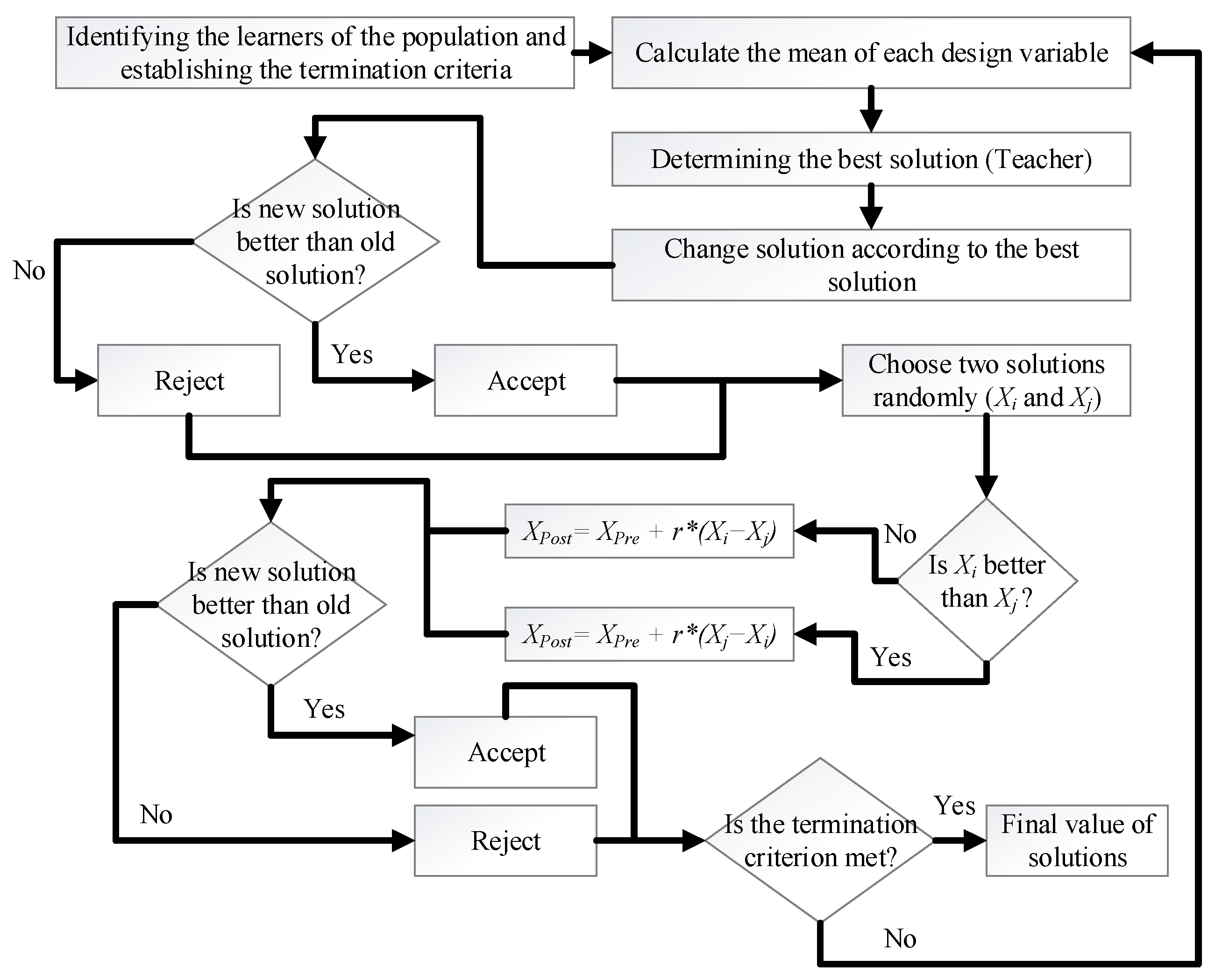
2.1. Teaching Learning Based Optimization (TLBO)

Teaching learning-based optimization (TLBO) is proposed by Rao et al. for optimization problems [26]. It is an optimization algorithm based on the teacher’s work to raise the level of the class and the level of the students triggered by supporting each other. The method consists of two parts: teaching and learning. The most successful student in the class becomes the teacher, then the chosen student and the teacher interact to make the randomly selected student-level approach the teacher level (Figure 1). The second stage aims to increase the students’ level by ensuring their interaction [26].

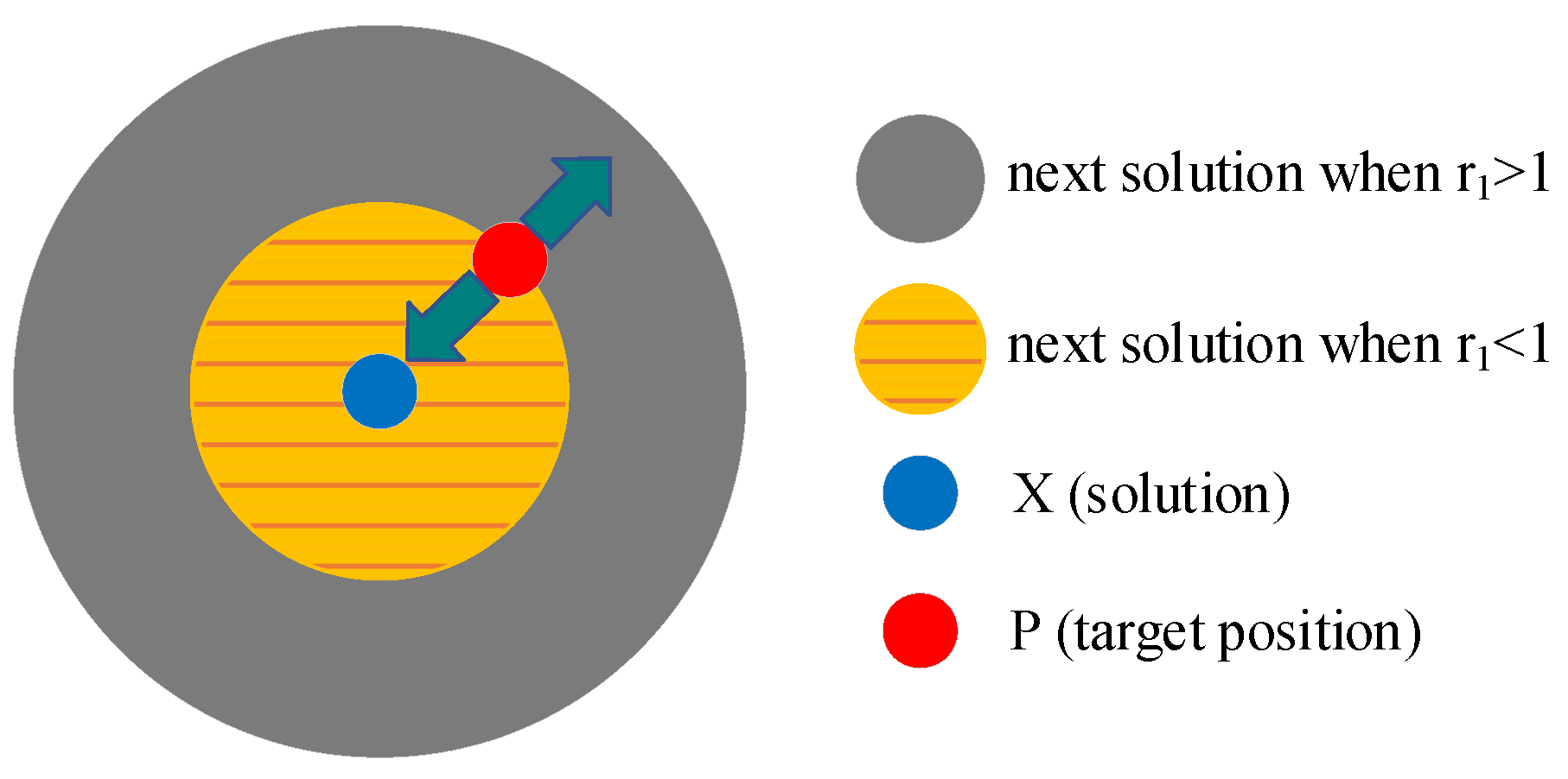
2.2. Sine Cosine Optimization Algorithm (SCO)

The sine cosine algorithm (SCA) is a trigonometry-based optimization algorithm developed by Mirjalili using sine and cosine [24]. Initially, SCA generates solutions based on multiple random variables whose orientation is either close or far from the objective function. Random and adaptive variables are added to the algorithm to strengthen the discovery and exploitation steps. The mentioned features are added in the following equations [24].

$$x_i^{t+1}=\{\begin{array}{c}{x}_i^t+r_1\sin (r_2)·\left|r_3 P_i^t-x_i^t\right|, r_4<0.5 \\ x_i^t+r_1\cos \left(r_2\right)·\left|r_3{P}_i^t-x_i^t\right|, r_4\ge 0.5\end{array}$$

(1)

In this equation, $P_i^t$ is the target position of the i-th dimension in the t-th cycle, $x_i^t$ is the position of the i-th dimension in the t-th cycle, $r_1$ is the randomly generated number as the next position factor. $r_2$ is the randomly generated factorial number used to determine whether the movement will be towards or away from the target. $r_3$ is a randomly generated factorial number to create the weight for the target. It either makes the distance to the target value more important ($r_{3 }$> 1) or less critical ($r_{3 }$< 1). $r_4$ is randomly generated in the range [0, 1]. Depending on the value it takes, either cosine or sine is used in the equation.

The effects of the functions in Equation (1) for the next position are shown in Figure 2.

To balance exploration and exploitation stages, Equation (2) is used as well. Here, a is constant, T is the maximum number of cycles, and t is the current cycle. Sine and cosine search different regions depending on whether they are greater or less than one. It returns when it takes values between −1 and 1 close to the objective function [24].

$$r_1=a-t\frac{a}{T}$$

(2)

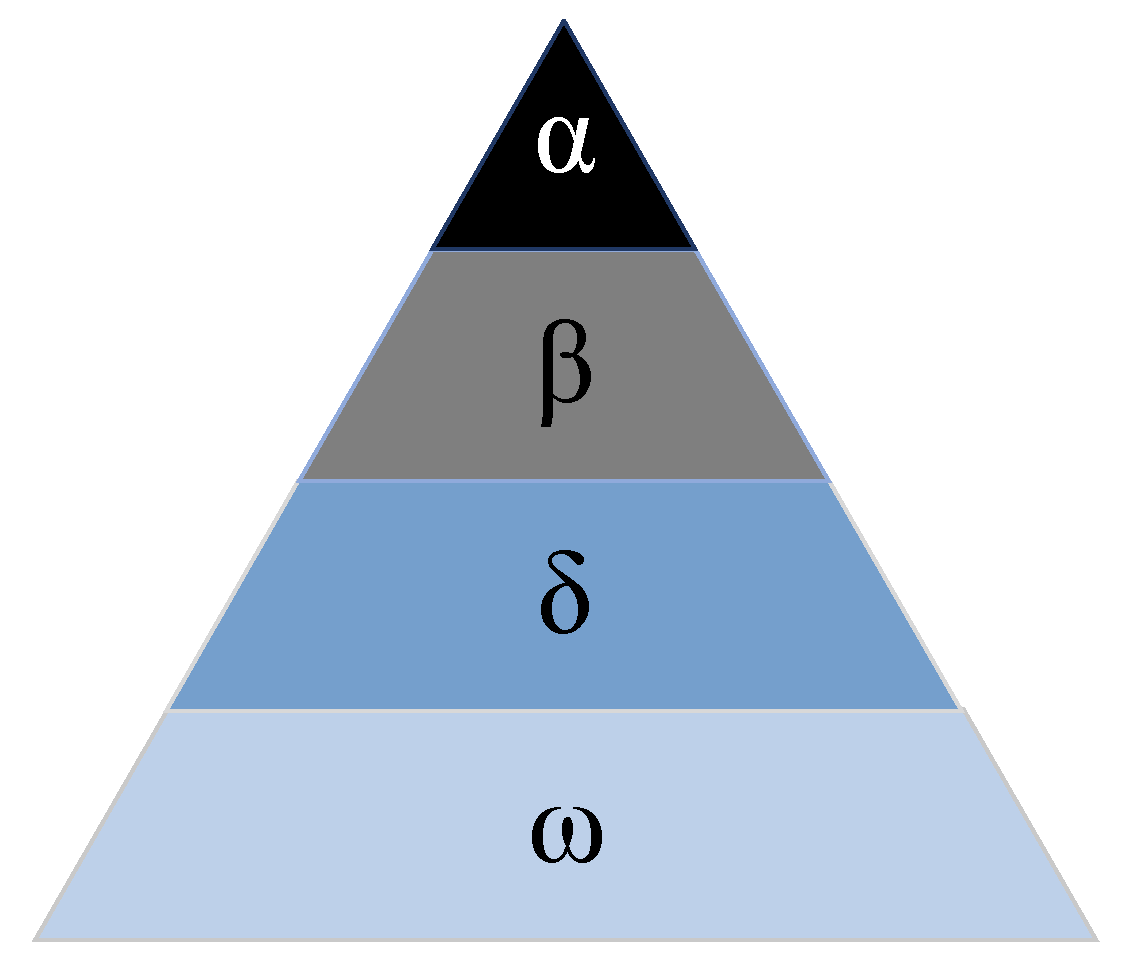
2.3. Gray Wolf Optimization Algorithm (GWO)

The gray wolf optimization (GWO) algorithm is an optimization algorithm inspired by the life and hunting of gray wolves [27,28]. There is a hierarchical structure in which the alpha wolves are superior in the pack structure of the gray wolves, followed by the beta, delta, and omega wolves (Figure 3). These three wolfs are for hunting, searching, and attacking, respectively.

2.3.1. Hunting

The process performed in hunting is shown below, respectively.

• Monitoring, tracking, and approaching the prey.
• Surrounding the prey and moving it until the prey is tired.
• Performing an attack on the prey.

Equations (3) and (4) are applied to contain the prey in the GWO algorithm. In these equations, t is the instantaneous cycle number, $X_p$ is the hunting position, and X is the current wolf’s position vector. A and C are vector coefficients. $\overrightarrow{D}$ is the position update vector.

$$\overrightarrow{D}=\left|C \overrightarrow{X_p\left(t\right)}-\overrightarrow{X\left(t\right)}\right|$$

(3)

$$\overrightarrow{X\left(t+1\right)}=\overrightarrow{X_p\left(t\right)}-A \overrightarrow{D}$$

(4)

In Equations (5) and (6), the calculation of vectors A and C is done.

$$A=a \left(2 r_1-1\right)$$

(5)

$$C=2 r_2$$

(6)

Here, the number of random factors $r_1$ and $r_2$ generated between [0, 1] are increasing coefficients as the iteration progresses from two to zero.

2.3.2. Exploration

In GWO, the search starts randomly. Then, the fitness of each wolf is calculated according to the objective function. The top three values that give the best cost are taken as alpha, beta, and delta worms, respectively. Alpha wolf is the best solution in the GWO algorithm. Beta is the second, and delta is the third-best solution. The omega wolf is also a candidate solution. The alpha wolves lead the hunt, and beta and delta wolves join when necessary. The positions of the wolves are updated as follows.

$$D_{\alpha }=\left|C_1 X_{\alpha }-X\left(t\right)\right|, D_{\beta }=\left|C_1 X_{\beta }-X\left(t\right)\right|, D_{\delta }=\left|C_1 X_{\delta }-X\left(t\right)\right|$$

(7)

Here, $X_{\alpha }$,$X_{\beta }$, and $X_{\delta }$ denote the positions of the wolves. The best wolves are updated with each iteration. Here, $x_1$, $x_2$, and $x_3$ are the updated positions of the three best wolves (Equation (8)).

$$x_1=\left|X_{\alpha }-{\alpha }_1 D_{\alpha }\right|, x_2=\left|X_{\beta }-{\alpha }_2 D_{\beta }\right|, x_3=\left|X_{\delta }-{\alpha }_1 D_{\delta }\right|$$

(8)

Then, the average of these three wolves is taken, and the new position of the prey, $X\left(t+1\right)$, is obtained (Equation (9)).

$$X\left(t+1\right)=\frac{X_1+X_2+X_3}{3}$$

(9)

2.3.3. Attack

In GWO, the location of the prey is determined, then the prey is attacked. The attack occurs when the prey gets tired and its movement stops. Mathematically, the attack occurs according to A’s value in the models. The value of A decreases from two to according to the random variable $r_1$. In this case, variable A takes values in the range [−2a, 2a]. If A is greater than one, the wolves do not approach the prey and start looking for the more suitable one. If A is less than one, the prey is attacked. In the GWO, hunting continues until the stop criterion.

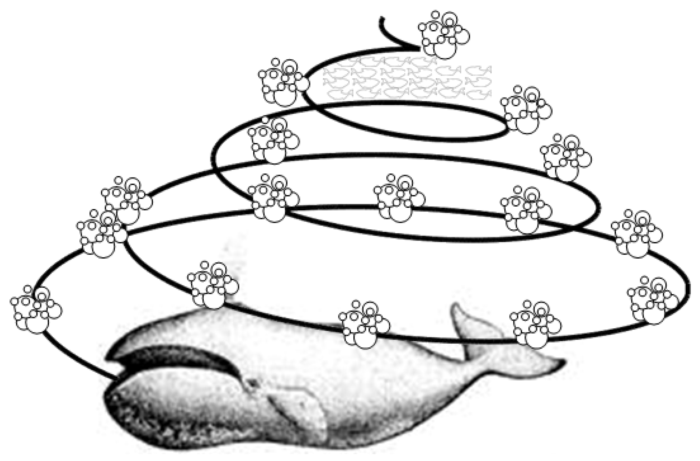
2.4. Whale Optimization Algorithm (WO)

The WOA algorithm was proposed by Seyedali Mirjalili and Andrew Lewis in [28]. WOA is a metaheuristic algorithm inspired by the hunting of humpback whales. Humpback whales produce spiral-shaped bubbles that narrow upward when they hunt (Figure 4) [28].

2.4.1. Surrounding Prey

In WOA, the hunt is considered the optimum point to reach. Since we do not know the most appropriate point in optimization, the optimum point is taken as the current best point or a point around it. After determining the current optimum solution, other solutions are compared with the optimum solution, which is updated. This situation is shown in Equations (10) and (11).

$$\overrightarrow{D}=\left|\overrightarrow{C} \overrightarrow{X^{*}}\left(t\right)-\overrightarrow{X_t}\right|$$

(10)

$$\overrightarrow{X}\left(t+1\right)=\overrightarrow{X^{*}}\left(t\right)-\overrightarrow{A} \overrightarrow{D}$$

(11)

Here, t is the number of iterations, $\overrightarrow{A}$ and $\overrightarrow{C}$ are the coefficient vectors, $\overrightarrow{X^{*}}$ is the current best state vector, and $\overrightarrow{X}$ is the relevant search agent state vector. At the end of each iteration, $\overrightarrow{X^{*}}$ is checked to see if there is a better vectors solution than $\overrightarrow{X^{*}}$. If a better solution is found, $\overrightarrow{X^{*}}$ is updated. The equations used to calculate the coefficient vector $\overrightarrow{A}$ and $\overrightarrow{C}$ are as Equations (12)–(14).

$$\overrightarrow{A}= 2\overrightarrow{a} \overrightarrow{r-\overrightarrow{a}}$$

(12)

$$\overrightarrow{c}=2 \overrightarrow{r}$$

(13)

$$\overrightarrow{a}=2-m(2/M)$$

(14)

$\overrightarrow{r}$ is randomly generated in the interval [0, 1]. $\overrightarrow{a}$ decreases linearly from two to zero over the iteration. M shows the maximum iteration, whereas m is the current iteration value.

2.4.2. Attacking the Prey Using a Bubble-Net Method

The bubble-net method is modeled in two parts: the narrowing the circle around the prey and the spiral movement. Narrowing the circle around prey is achieved by linearly decreasing the value of 𝑎 in Equation (14). The spiral motion is modeled by Equations (15) and (16) [29].

$$\overrightarrow{X}\left(t+1\right)=\overrightarrow{D\prime } e^{bl} \cos \left(2\pi l\right)+\overrightarrow{X^{*}}\left(t\right)$$

(15)

$$\overrightarrow{D\prime }=\left|\overrightarrow{X^{*}}\left(t\right)-\overrightarrow{X}\left(t\right)\right|$$

(16)

$\overrightarrow{D\prime }$ in the equation is the distance between the search agent and the best location. b is the logarithmic spiral constant, and 𝑙 is a random number in the [−1, 1] range. The spiral movement continues as it heads towards the hunt. In the algorithm, the determination of the movement type, such as towards the spiral or hunt, is made with a probability of 0.5, as in Equation (17). Here, p is the random number [30].

$$\overrightarrow{X}\left(t+1\right)=\{\begin{array}{cc}\hfill \overrightarrow{X^{*}}\left(t\right)-\overrightarrow{A} \overrightarrow{D},& p<0.5\hfill \\ \hfill \overrightarrow{D\prime } e^{bl} \cos \left(2\pi l\right)+\overrightarrow{X^{*}}\left(t\right) ,& p\ge 0.5\hfill \end{array}$$

(17)

2.4.3. Prey Exploration (Global Searching)

For global searches, the new states of their agents are determined by the randomly selected search agent rather than the best-known state. Global searching is shown in Model Equations (18) and (19). In the equations, $\overrightarrow{X_{rand}}$ is the randomly picked search agent [28].

$$\overrightarrow{D\prime }=\overrightarrow{C } \overrightarrow{X_{rand}}-\overrightarrow{X}$$

(18)

$$\overrightarrow{X}\left(t+1\right)=\overrightarrow{X_{rand}}-\overrightarrow{A} \overrightarrow{D}$$

(19)

The value of A indicates whether it will be a global or a local search. Since A > 1 or A < −1, a situation far from the best situation can be selected, this situation is accepted as a global search, and the new state of the individual is calculated with Equation (19) instead of Equation (11).

2.5. Salp Swarm Optimization Algorithm (SSO)

Salp has to pump water through its body to move forward, and it is an algorithm inspired by swarms of seaweed that feed on plankton [29]. Chains link their bodies, and they feed together. There is a structure in the form of a leader and followers in the salp flock. SSA defines the best solution as food. The leader salp investigates the equilibrium state between the convergence state and the search in the algorithm. Leader salp updates the status based on the best result food. Since the followers are chained, they automatically update their positions. This gradual convergence prevents catching on local optimal and early convergence [29].

The leading salp position is given in Equation (20). In this equation, $X_j^1$ is the position of the leading scallop in the j-th dimension, $F_j$ is the food source position in the j-th dimension, $c_1$, $c_2$, $c_3$ are random numbers, $u_{bj}$ is the upper bound in the j-th dimension, and $l_{bj}$ is the j-th dimensional indicating the lower limit. The leading position in Equation (20) is only updated towards the food source.

$$X_j^1=\{\begin{array}{c}{F}_j+c_1\left(\left(u_{bj}-l_{bj}\right) c_2+l_{bj}\right), c_3\ge 0\\ F_j+c_1\left(\left(u_{bj}-l_{bj}\right) c_2+l_{bj}\right), c_3<0\end{array}$$

(20)

$c_1$ is the most critical parameter in the SSA algorithm. Because $c_1$, shown in Equation (21), determines the balancing of exploration and exploitation [31].

$$c_1=2e^{{\left(-\frac{4l}{L}\right)}^2}$$

(21)

I in Equation (21) shows the current iteration, and L is the maximum iteration. The parameters $c_2$,$c_3$ are random numbers in the [0, 1] range. The update in Equation (22) is applied to the positions of the followers.

$$X_j^i=\frac{1}{2}a{t}^2+v_{0}t$$

(22)

If i ≥ 2, $X_j^i$ is the j-th size and i-th follower salps position. t is the time, $v_0$ is the initial velocity. a in Equation (22) is the $v_{\mathit{final}}/v_0$ ratio. $X_0$ is the initial position, X is the current position, and $v$ is the current velocity. They are equal to $a=\frac{v_{final}}{v_0}$ and $v=\frac{X-X_0}{t}$.

Equations (20) and (23) are used to simulate the algorithm to the salp chain structure.

$$X_j^i=\frac{1}{2}\left(X_j^i+X_j^{i-1}\right)$$

(23)

The general workflow of SSO is as follows. In a search space with a fixed or mobile food source and a chain of multiple salps, the leading salp changes position around the food source, and the follower salps gradually follow the leader salp through iterations.

2.6. Harris Hawk Optimization Algorithm (HHO)

It is an optimization algorithm based on swarm intelligence inspired by Harris hawks, which are desert hawks, by Heidari et al. [31]. Harris hawks pursue their prey cooperatively [32]. Harris hawks try to confuse prey and attack together. Harris hawks choose the type of chase according to the escape status of the prey [32]. The Harris hawk moves by using its herd intelligence, especially when hunting rabbits. First, the leader and remaining herd members take priority and make a reconnaissance flight. After the prey is detected, the hunt begins. Harris hawks trap their prey through exploration and operation phases.

2.6.1. Exploration Phase

Harris hawks can see their prey with their sharp eyes. Sometimes they may not easily spot prey. Harris hawks wait in the desert and make pancakes in such a case. This situation continues cyclically. The results obtained in these cycles are the Harris hawks candidate solutions. The optimal solution is the hawk closest to the prey in each cyclical operation. Harris hawks perform two scouting methods when roaming randomly in areas. These are shown in Equation (24). Here, 𝑞 is the probability value determining which application is active [31,33].

$$x\left(t+1\right)=\{\begin{array}{cc}\hfill x_{rand}\left(t\right)-r_1\left|x_{rand}\left(t\right)-2r_{2}x\left(t\right)\right|,& q\ge 0.5\hfill \\ \hfill \left(x_{rabbit}\left(t\right)-x_m\left(t\right)\right)-r_3\left(LB+r_4\left(UB-LB\right)\right),& q<0.5\hfill \end{array}$$

(24)

$x\left(t+1\right)$ is the Harris hawk position vector at each iteration. $x_{rabbit}\left(t\right)$ is the prey position vector, $x\left(t\right)$ is the hawk’s current position, and $r_1$, $r_2$, $r_3$, $r_4$, and q are random numbers generated between [0, 1]. LB and UB are lower and upper bounds, respectively. $x_{rand}\left(t\right)$ is the randomly selected hawk from the flock. $x_m\left(t\right)$ is the average position of the current hawk flock. The average position is given in Equation (25).

$$x_m\left(t\right)=\frac{1}{N}{{\displaystyle \sum }}_{i=1}^N{x}_i\left(t\right)$$

(25)

Here, 𝑁 denotes the number of hawks, where 𝑡 is the number of iterations.

2.6.2. Transition from the Exploration Phase to the Attack Phase

Harris hawks plan different attacks depending on the energy of the prey. During the escape, the energy of the prey is significantly reduced. The mathematical model of this situation is given in Equation (26) [31,33]. In this equation, E is the energy of the escaped prey, $E_0$ is the initial energy of the prey, and 𝑇 is the maximum iteration value.

$$E=2E_0\left(1-\frac{t}{T}\right)$$

(26)

2.6.3. Attack Phase

At this stage, the Harris hawk launches an attack. It demonstrates a surprise leaping action. The prey tries to get rid of this situation. According to the movement of the prey, the Harris hawk responds with the appropriate strategy. The situation mentioned in the algorithm is done in four different ways [31].

• Soft siege: The Harris hawk tries to de-energize its prey with false moves at this stage.

(r ≥ 0.5, E ≥ 0.5). The equations of this siege in (27) and (28) are as follows.

$$x\left(t+1\right)=∆x\left(t\right)-E\left|J x_{rabbit}\left(t\right)-x\left(t\right)\right|$$

(27)

$$∆x\left(t\right)=x_{rabbit}\left(t\right)-x\left(t\right)$$

(28)

Here, r is the probability that the rabbit is prey, and E is the energy state of the rabbit. In $∆x\left(t\right)$, 𝑡 is the difference between their position in the iteration and the rabbit’s position. J is the changing value at each iteration [32,33] to simulate the movements of rabbits in nature.

• Hard siege: At this stage, the prey’s energy is quite depleted (r ≥ 0.5, |E| ≤ 0.5). The hawk hardly flanks to snatch its surprise claw on the hunt. This siege is shown in Equation (29) [31,33].

$$∆x\left(t\right)=x_{rabbit}\left(t\right)-E\left|∆x\left(t\right)\right|$$

(29)

• Soft siege with progressive rapid dives: The prey has the energy to escape at this stage. The Harris hawk is still in soft encirclement before making a surprise leap. This stage is wiser than the previous stage. The following action to be taken before the hawks make the soft siege is given in Equation (30).

$$Y=x_{rabbit}\left(t\right)-E\left|x_{rabbit}\left(t\right)-x\left(t\right)\right|$$

(30)

This move is then compared with the last move to be able to decide on the status of this move. If it is decided that the situation is not suitable, the hawks take a quick dive into their prey. During the decision, the hawk moves using a Levy flight-based structure. This situation is given below.

$$Z=Y+S LF\left(D\right)$$

(31)

Here, D is the problem dimension, S is the randomly generated vector with the size of 1 × D, Y is the position of the prey due to decreasing energy; Z is the LF levy function, which allows deciding whether the hawk will move toward the hunt or not. The situation is given in the following equation.

$$LF=0.01 \frac{u \sigma }{{\left|v\right|}^{\frac{1}{\beta }}} , \sigma ={(\frac{\tau \left(1+\beta \right)\sin \frac{\pi \beta }{2}}{\tau \left(\frac{1+\beta }{2}\right) \beta 2^{\left(\frac{\beta -1}{2}\right)}})}^{\frac{1}{\beta }}$$

(32)

Here, 𝑢 is the random number generated between 𝑣 (0, 1), and 𝛽 is 1.5. The following Equation (33) is used to update the positions of the hawks during the soft encirclement phase.

$$x\left(t+1\right)=\{\begin{array}{c}Y if F\left(Y\right)<f\left(x\left(t\right)\right)\\ Z if F\left(Z\right)<F\left(x\left(t\right)\right)\end{array}$$

(33)

• Hard siege with progressive rapid dives: The prey has no energy to escape at this stage. Hawk makes a hard siege before his surprise leap to catch the prey. This situation is shown in Equations (34)–(36) [31,32].

$$x\prime \left(t+1\right)=\{\begin{array}{c}Y\prime if F\left(Y\prime \right)<f\left(x\left(t\right)\right)\\ Z\prime if F\left(Z\prime \right)<F\left(x\left(t\right)\right)\end{array}$$

(34)

$$Y^{\prime }=x_{rabbit}\left(t\right)-E\left|x_{rabbit}\left(t\right)-x_m\left(t\right)\right|$$

(35)

$$Z^{\prime }=Y^{\prime }+S LF\left(D\right)$$

(36)

3. Modeling

The thermal boundary layer is the flow region above the surface where temperature changes in the surface’s normal direction are significant. The thermal boundary layer thicknesses increase in the direction of the flow. This situation is because the efficiency of heat transfer decreases in the direction of the flow. In this part, the boundary layer thickness is determined by optimization algorithms for laminar zone airflow where characteristics are constant, irradiation is neglected, and plate and air temperature are constant in a steady regime. The properties of the air in atmospheric pressure are given in

Table 1. $\rho , v, k, c_p$ values of air at 80 °C and 100 °C.

$\mathbf{A}\mathbf{i}\mathbf{r}$	$80 °\mathbf{C}$	$100 °\mathbf{C}$
$\rho \left(\frac{kg}{m^3}\right)$	$0.999$	$0.9458$
$v \left(\frac{m^2}{s}\right)$	$20.94\times {10}^{-6}$	$23.06\times {10}^{-6}$
$k \left(\frac{W}{mK}\right)$	$~0.031$	$~0.031$
$c_p \left(\frac{J}{kgK}\right)$	$1009$	$1011$

.

In this problem, laminar flow occurs if $Re<5\times {10}^5$. Equation (37) is used to calculate the Re number.

$$R{e}_x=\frac{u_{\infty }x}{v}=\frac{\mathsf{\rho }{u}_{\infty }x}{\mu }$$

(37)

Here, $u_{\infty }$ is air-free flow rate, x is the distance from the leading edge, and υ is the kinematic viscosity of the fluid. The Prandal value given in Equation (38) needs to be calculated in the next step.

$$Pr=\frac{v}{\alpha }=\frac{v}{\frac{k}{\rho c_p}}$$

(38)

In this equation, $c_p$ is the specific heat at constant pressure (kJ/(kg°C)), k is thermal conductivity (W/(m°C)), α is thermal spread, and ν is the kinematic viscosity. The Nusselt number is calculated in Equation (39) using Pr and Re values.

$$N{u}_x=0.332R{e}^{1/2}P{r}^{1/3}$$

(39)

Here, Re is the Reynolds number, Pr is the Prandtl number, and Nu is the Nusselt number.

Nu number is used in the calculation of the heat transfer coefficient h. The heat transfer coefficient is calculated over Equation (40) by using Nu, k, and x.

$$h=\frac{N{u}_{x}k}{x}, \overline{h}=2h$$

(40)

The heat flux equation, including the obtained heat transfer coefficient, is defined in Equation (41).

$$Q=\overline{h}A\left(T_w-T_{\infty }\right)$$

(41)

where h is the heat transfer coefficient, $\overline{h}$ is the average value of the heat transfer coefficient, x is the distance from the leading edge, $T_w$ is the internal temperature and $T_{\infty }$ is the outside temperature. Here, A is the plate area and product of the width and the length. The thermal boundary layer thickness is calculated in Equation (42) using Re, Pr, and x values.

$$\delta =\frac{4.64}{\sqrt{R{e}_x}}x, {\delta }_t=\frac{0.977}{P{r}^{1/3}}\delta$$

(42)

In this equation, $\delta$ is hydrodynamic boundary layer thickness, ${\delta }_t$ is the thermal boundary layer thickness.

If $R{e}_x=\frac{u_{\infty }x}{v}=\frac{\mathsf{\rho }{u}_{\infty }x}{\mu }>5\times {10}^5$, a transition from laminar to turbulent flow takes place. Here, $u_{\infty }$ is air free flow velocity, x is the distance from the leading edge, and μ/ρ is the kinematic viscosity modeling, as shown in Figure 5.

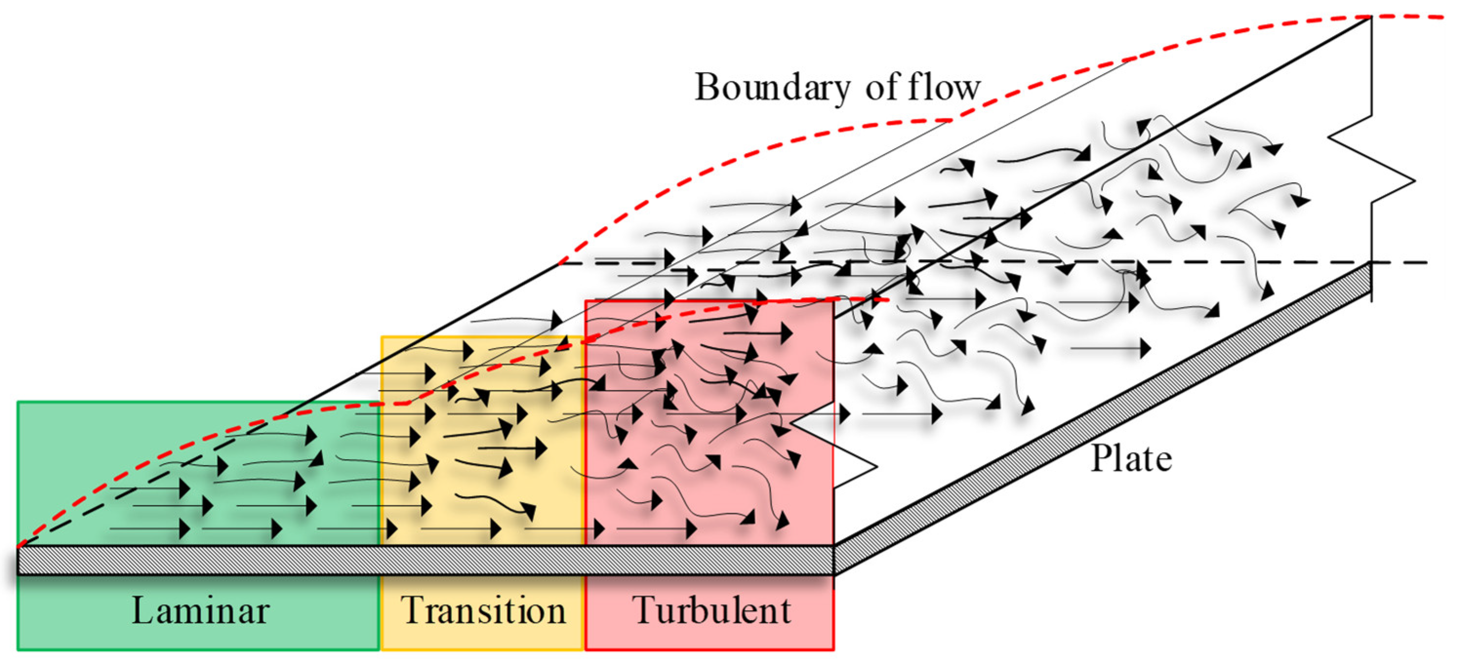
3.1. Sample Problem for Linear Flow

Assume that air at a temperature of 56.5 °C under 1 bar pressure flows at a velocity of 4.5 m/s over a 1 × 0.8 m plate with a temperature of 124.5 °C. In this problem when:

• Local heat transfer coefficient at a distance of 0.4 m and 0.8 m from the beginning of the plate, the arithmetic average of the heat transfer coefficient of the plate,
• The heat flux from the plate to the air,
• Velocity at the end of the plate and thickness of the thermal boundary layer, are asked, and the solution is given below [34].

Firstly, for flow on the surface, the below is valid.

$$R{e}_x<5\times {10}^5 \to N{u}_x=0.332R{e}_x^{\raisebox{1ex}{$1$}\!\left/ \!\raisebox{-1ex}{$2$}\right.}P{r}^{\raisebox{1ex}{$1$}\!\left/ \!\raisebox{-1ex}{$3$}\right.}$$

(43)

$$R{e}_x>5\times {10}^5 \to N{u}_x=0.0296R{e}_x^{0.8}P{r}^{\raisebox{1ex}{$1$}\!\left/ \!\raisebox{-1ex}{$3$}\right.}$$

(44)

The density, kinematic viscosity, thermal conductivity coefficient, and specific air heat at 80 °C and 100 °C are given in Table 1. The solution will be realized using these values.

The assumptions in this problem are listed below.

• Continuous regimen,
• Neglecting the radiation,
• The properties, temperature values of the plate, and the air are fixed.

The average air temperature between the plate and out-of-boundary flow is given below.

$$T_f=\frac{T_{\infty }+T_y}{2}=\frac{56.5+124.5}{2}=90.5°\mathrm{C}$$

(45)

when the density, kinematic viscosity, and specific heat of the air at constant pressure are found using linear interpolation with Table 1 for 90.5 °C, these values are respectively υ = 22.04 × 10⁻⁶ m²/s, ρ = 0.971 kg/m³, c_p = 1010 J/(kgK). Then, using Equation (38), the Pr value is calculated as in Equation (46);

$$Pr=\frac{v}{\alpha }=\frac{v}{\frac{k}{p{c}_p}}=\frac{22.04\times {10}^{-6}}{\frac{0.031}{0.971\times 1010}}\cong 0.70$$

(46)

Re and Nu numbers are calculated by using Equations (37) and (38) for the calculation of heat convection coefficient at $x_1=0.4 \mathrm{m}$ and $x_2=0.8 \mathrm{m}$ asked in option a.

$$R{e}_{0.4}=\frac{u_{\infty }{x}_1}{v}=\frac{4.5\times 0.4}{22.04\times {10}^{-6}}=81,669.7<5\times {10}^5$$

(47)

$$R{e}_{0.8}=\frac{u_{\infty }{x}_2}{v}=\frac{4.5\times 0.8}{22.04\times {10}^{-6}}=163,339.4<5\times {10}^5$$

(48)

Since $R{e}_{0.4}<5\times {10}^5$ as a result of Equations (15) and (16), the first relation is obtained. The Nu value is shown in Equations (49) and (50) for x = 0.4 m and Equations (51) and (52) for x = 0.8 m.

$$N{u}_{0.4}=0.332 R{e}_{0.4}^{1/2} P_r^{1/3}=0.332 {\left(81,669.7\right)}^{1/2} {\left(0.70\right)}^{1/3}=84.25$$

(49)

$$N{u}_{0.4}=\frac{h_{0.4}{x}_1}{k} \to h_{0.4}=\frac{N{u}_{0.4}k}{x_1}=\frac{84.25\times 0.031}{0.4} h_{0.4}=6.53 \mathrm{W}/{\mathrm{m}}^2\mathrm{K}$$

(50)

and

$$N{u}_{0.8}=0.332 R{e}_{0.8}^{1/2} P_r^{1/3}=0.332{\left(163,339.4\right)}^{1/2}{\left(0.70\right)}^{1/3}=119.15$$

(51)

$$N{u}_{0.8}=\frac{h_{0.8}{x}_2}{k} \to h_{0.8}=\frac{N{u}_{0.8}k}{x_2}=\frac{119.15\times 0.031}{0.8} h_{0.8}=4.62 \mathrm{W}/{\mathrm{m}}^2\mathrm{K}$$

(52)

The arithmetic average of the heat transfer coefficient of the plate asked in option a is two times the value found at the end of the plate. According to this;

$$h=\overline{h}=2h_{0.8}=\left(2\right) \left(4.62\right) \to h=9.24 \mathrm{W}/{\mathrm{m}}^2\mathrm{K}$$

(53)

The heat flux that reaches the air by convection from the plate asked in option b is calculated by Equation (41).

If h, A, and temperature are substituted in the equation, the result is found in Equation (54).

$$Q=\left(9.26\right)\left(1\right)\left(0.8\right)\left(124.5-56.5\right), Q=503.7 \mathrm{W}$$

(54)

The thicknesses of the velocity (δ) and thermal boundary (δ_t) layer at the end of the plate ($x_2=0.8 m$) are given in Equations (55) and (56), respectively;

$$\frac{\delta }{x_2}=\frac{5}{\surd R{e}_{0.8}} \to \frac{\delta }{0.8}=\frac{5}{\surd 163,339.4} , \delta =0.0099 \mathrm{m}=9.9 \mathrm{mm}$$

(55)

$$\frac{{\delta }_t}{\delta }=\frac{0.974}{P{r}^{1/3}} \to \frac{{\delta }_t}{0.0099}=\frac{0.974}{{0.70}^{1/3}}, {\delta }_t=0.0108 \mathrm{m} \cong 10.8 \mathrm{mm}$$

(56)

As a result of the processes, the thicknesses of the velocity (δ) and thermal boundary (δ_T) layer at the end of the plate ($x_2=0.8 \mathrm{m}$) are determined as 9.9 mm and 10.8 mm, respectively.

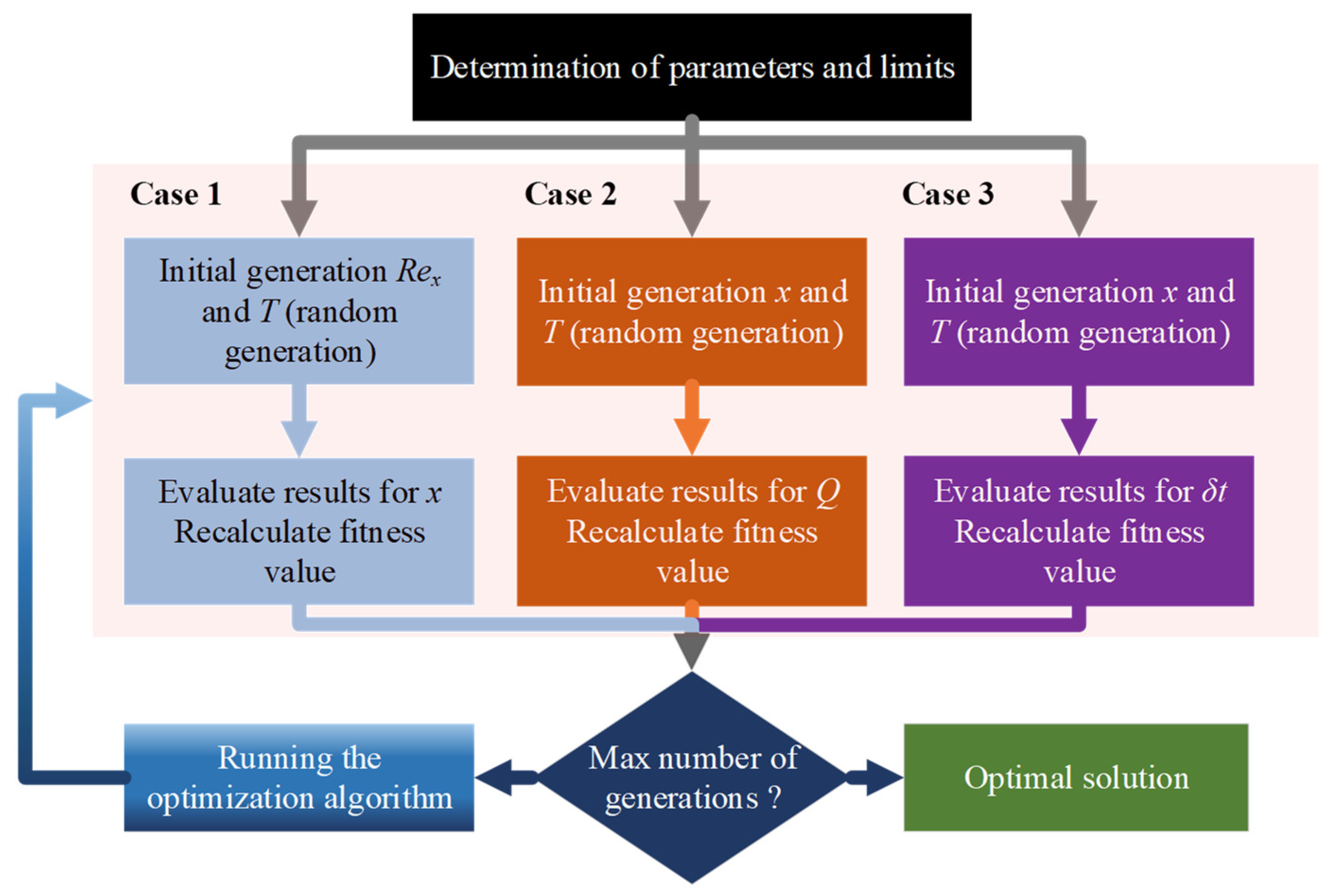
3.2. Sample Cases for Linear Flow

In the critical thickness problem of the thermal boundary layer for laminar flow, three different cases were examined, and their optimization was achieved. These three situations are targeted as follows:

• The thermal boundary layer thickness (${\delta }_t$),
• The heat flux (Q),
• The distance (x) from the edge.

Details of these situations are given in the next paragraph. The flow diagram of the six optimization algorithms is given in Figure 6.

The first case is shown as “Case 1”. This case is used to verify the correctness of the adopted calculation methodology. Here, the goal is to determine the maximum, minimum, and target (0.61 m) values of the distance (x) from the leading edge. The constraints for this case are the variables Q (140 W ≤ Q ≤ 190 W) and ${\delta }_t$ (0.01 mm ≤ ${\delta }_t$ ≤ 28 mm). In addition, the design variables in the model are the Reynolds number (0.01 ≤ $R{e}_x<50\times {10}^3$)) and temperature T (80 °C ≤ T ≤ 130 °C), respectively. T is the average temperature that is calculated as T_f in Equation (45). The design variables in the initial states of the optimization algorithms are $R{e}_x$ = 1, T = 1 °C, respectively.

In “Case 2”, the goal is to determine the maximum, minimum, and target (160.43 W) values of the heat flux (Q). In Case 2, while the constraint is reduced by one, the number of design variables is increased by one. In Case 2, the constraint is the variable Re ($R{e}_x<50\times {10}^3$). The design variables in the model are the distance from the edge x (0.02 m ≤ x ≤ 1 m), the temperature T (80 °C ≤ T ≤ 130 °C), and the thermal boundary layer thickness ${\delta }_t$ (0.01 mm ≤ ${\delta }_t$ ≤ 20 mm). The design variables in the initial states of the optimization algorithms are x = 1 m, T = 1 °C, ${\delta }_t$ = 1 mm, respectively.

In “Case 3”, the goal is to determine the maximum, minimum, and target (19.6 mm) values of the thermal boundary layer thickness (${\delta }_t$). The constraints for this case are the variables of Re ($R{e}_x<50\times {10}^3$) and Q (140 W ≤ Q ≤ 190 W). In addition, the design variables in the model are the distance from the edge x (0.02 m ≤ x ≤ 1 m) and the temperature T (80 °C ≤ T ≤ 130 °C), respectively. T is the average temperature that is calculated as T_f in Equation (45). The design variables in the initial states of the optimization algorithms are x = 1 m and T = 1 °C, respectively.

One hundred populations, 100 iterations, and 10 random tests with the same initialization values are performed in the six optimization algorithms used in all three cases.

The objective function of Case 1 is determined by the distance from the edge and leaving the x in Equation (37) alone. The related equation is shown in Equation (57). In this equation, υ is the kinematic viscosity of the fluid and is determined using Table 1 using linear interpolation (Equation (58)).

$$x=\frac{R{e}_x\upsilon }{U_h}$$

(57)

$$v={\nu }_{min}+\left({\nu }_{max}-{\nu }_{min}\right) \left(\frac{T_f-T_{min}}{T_{max}-T_{min}}\right)$$

(58)

$R{e}_x$, T, ${\delta }_t$, and Q values, which enable the best result to be produced according to the determined state of the objective function (minimum-maximum-target value), are determined by optimization algorithms, and the optimum function (x) value is found.

The objective function in Case 2 is heat flow, shown in Equation (40). $R{e}_x$, T, ${\delta }_t$, and x values, which enable the best result to be produced according to the determined state of the objective function (minimum-maximum-target value), are determined by optimization algorithms, and the optimum function (Q) value is found.

The objective function in Case 3 is the boundary layer thickness shown in Equation (42). $R{e}_x$, T, Q, and x values, which enable the best result to be produced according to the determined state of the objective function (minimum-maximum-target value), are determined by optimization algorithms, hence the optimum function (${\delta }_t$) value is found.

4. Results

This study used six different optimization algorithms to solve the laminar flow problem. In the problem, three different situations are demonstrated for three distinct variables. Ten tests are repeated at long intervals to avoid misleading results caused by reading the cache. MATLAB R2020a is used as the software environment. The number of iterations and the population sizes are 100 in all algorithms. The results of the studies carried out are shown in this section.

In the thermal boundary layer problem of Case 1, in determining the maximum, minimum, and target (0.61 m) distance from the leading edge (x), the design variables are 0.01 ≤ Re_x ≤ 50 × 10³, 80 °C ≤ T ≤ 130 °C, while the constraints are 0.02 m ≤ x ≤ 1 m was 140 W ≤ Q ≤ 190 W, 0.01 mm ≤ δ_t ≤ 28 mm.

Table 2. Case 1 optimization results, (a) x Minimum value, (b) x Maximum value, (c) x Target value (0.61 m).

(a)
Test	x	T	Rex	δt	Q	Time (s)	Error (%)
TLBO	0.08447	80	3843.735	7.073	189.9772	1.643198	0.0248671
SCO	0.08448	80	3844.1874	7.0734	189.966	1.0632657	0.0367085
GWO	0.084452	80	3842.9436	7.0723	189.9967	0.1437	0.0035524
WO	0.084449	80	3842.8114	7.0721	190	0.343593	0
SSO	0.084449	80	3842.8115	7.0721	190	1.01691	0
HHO	0.084449	80	3842.8114	7.0721	190	0.348538	0
(b)
Test	x	T	Rex	δt	Q	Time (s)	Error (%)
TLBO	1.2266	122.5319	50,000	27.9605	190	4.775296	0
SCO	1.2263	122.43045	50,000	27.95459	189.7014	2.37774	0.0244579
GWO	1.2266	122.5285	50,000	27.9603	189.98988	0.1356161	0
WO	1.2266	122.5319	50,000	27.9605	190	0.135099	0
SSO	1.2266	122.5319	50,000	27.9605	190	0.9328725	0
HHO	1.2266	122.5319	50,000	27.9605	190	0.2854132	0
(c)
Test	x	T	Rex	δt	Q	Time (s)	Error (%)
TLBO	0.610168	98.6629	26,416.801	19.3206	159.68272	4.594048	0.010248
SCO	0.6101	99.52021	26,353.486	19.33314	163.71016	2.425644	0.003477
GWO	0.6101	99.29481	26,368.825	19.3294	162.65995	0.148997	0.009344
WO	0.61	95.0744	26,659.71	19.2584	142.8026	0.1441	0
SSO	0.61	102.494	26,148.811	19.38185	177.62358	0.979427	0
HHO	0.61	97.78142	26,470.417	19.30326	155.56209	0.343977	0

a shows the minimum case results for Case 1. While WO, SSO, and HHO algorithms found error-free results in determining the minimum x value, the GWO algorithm found very close to zero error. While determining the minimum x, the T value of all algorithms is the same, where Re_x, δ_t, and Q values are very close to each other. In Table 2b, all algorithms reached the result without error except for the SCO algorithm for the maximum value of the distance (x) from the edge. The SCO algorithm error is determined as 0.024%. While all constraint and design variables of TLBO, WO, SSO, and HHO algorithms are able to find the same value, it is seen that there are minor differences in the T and Q values of the GWO algorithm. In the case where the distance from the edge is targeted (Table 2c), the WO, SSO, and HHO algorithms obtained error-free results. While SCO and GWO algorithms find the result with the same error value, it is seen that the constraint and design variables have slight differences. In the same case, the TLBO algorithm has the highest error. GWO, WO, and HHO algorithms have the shortest processing times.

The design variables are 0.02 m ≤ x ≤ 1 m, 80 °C ≤ T ≤ 130 °C, 0.01 mm ≤ δ_t ≤ 20 mm, and Re_x ≤ 50 × 10³ as the constraint in determining the maximum, minimum, and target (160.43 W) values of the heat flux (Q) is used in Case 2.

Table 3. Case 2 optimization results, (a) Q Minimum value, (b) Q Maximum value, (c) Q Target value (160.43 W).

(a)
Test	x	T	Rex	δt	Q	Time (s)	Error (%)
TLBO	0.158392	84.14076	8489.7097	12.35754	140.00307	1.86909	0.0021929
SCO	0.0814832	81.53445	3671.4047	10.61715	140.04808	1.1988065	0.0343429
GWO	0.477998	88.19405	21,313.158	15.05907	140.00393	0.163558	0.0028071
WO	0.661705	87.03197	29,459.85	14.28488	140.00005	0.253899	0.0000357
SSO	0.447057	84.06552	20,087.347	12.30769	140	1.1682	0
HHO	0.088826	90.91476	3916.7569	16.87286	140	0.552467	0
(b)
Test	x	T	Rex	δt	Q	Time (s)	Error (%)
TLBO	0.470381	98.87179	11,691.195	16.34188	189.9847	1.798275	0.0080526
SCO	0.26131	89.4444	11,656.033	11.71522	189.9228	1.1085021	0.0406316
GWO	0.61468	93.5664	26,766.681	13.73579	189.98671	0.1363648	0.0069947
WO	0.319576	102.6246	13,692.594	18.18359	189.9999	0.1592901	0.0000526
SSO	0.275089	96.42515	11,978.555	15.13887	190	1.1223129	0
HHO	0.30621	92.81981	13,365.664	13.36822	190	0.443047	0
(c)
Test	x	T	Rex	δt	Q	Time (s)	Error (%)
TLBO	0.430273	86.68083	13,681.897	12.26104	160.43663	1.830323	0.0041326
SCO	0.378001	88.67019	16,704.573	13.41592	160.46	1.1380122	0.0186997
GWO	0.451014	93.4736	19,813.337	16.21215	160.4334	0.190655	0.0021193
WO	0.3577	90.8456	15,862.732	14.6839	160.43	0.1707	0
SSO	0.363114	89.35783	16,097.652	13.81859	160.43	1.1523682	0
HHO	0.167105	88.45738	7352.8772	13.29482	160.43	0.476135	0

a shows the minimum case results for Case 2. While SSO and HHO algorithms found error-free results in determining the minimum Q value, the WO algorithm error rate is close to zero. The highest error occurred with SCO, which is 0.034%. GWO, WO, and HHO algorithms have the lowest processing time. Similar results to the minimum value are also obtained for the maximum heat flow value (Q), as shown in Table 3b. While SSO and HHO algorithms found the results without error, the WO algorithm determined the result with almost zero error. The highest error is determined in SCO with 0.04%. GWO is the lowest with 0.14 s, followed by WO with 0.16 s, while HHO is the third with 0.44 s. Other algorithms finished optimizing in less than a second. The situation where the target heat flow is specified is shown in Table 3c. While WO, SSO, and HHO algorithms found the target value without error, TLBO and GWO found the target value with an error of less than 0.005%. The situation regarding the processing times again showed that the three algorithms (GWO, SSO, HHO) found the result in a short time. The transition of the solution space caused the variables x, T, Re_x,, and δ_t to be different in all cases. For example, in determining the minimum Q value, while the SSO and HHO algorithms detected the heat flow without error, Re_x, x, T, and δ_t values took very different values from each other.

Case 2 is compared with Case 1 to verify the correctness of the adopted calculation methodology. While the minimum value of x in Case 1 is determined as 0.0844 m, the Q, T, Re, and δ_t values, in this case, are 190 W, 80 °C, 3842, and 7.07 mm, respectively. In Case 2, when SCO determined the minimum value of Q, the mean x value was found to be 0.815 m. In contrast to this value, the Q, T, Re, and δ_t values are 140 W, 81.5 °C, 3.671, and 10.61 mm, respectively. Again, when the target value of x in Case 1 is 0.61 m, it is seen that the Q, T, Re, and δ_t values are close to Case 2. For example, the WO results in Table 3a have x, T, Re, δ_t, and Q values of 0.66 m, 87 °C, 29.460, 12.28 mm, and 140 W, respectively, while the WO results in Table 2c have these values as 0.61 m, 95 °C, 26.659, 19.25 mm, and 142 W, respectively. Another similar example is seen in the GWO results in Table 3b, and the SSO results in Table 2c for Case 1. In the GWO results, x, T, Re, δ_t, and Q values are 0.61 m, 93.6 °C, 26.766, 13.7 mm, and 190 W, respectively, while in the SSO results, the x, T, Re, δ_t, and Q values are 0.61 m, 102.5 °C, 26.148, 19.38 mm, and 177 W, respectively. The two examples in Cases 1 and 2 showed that the results are consistent.

The constraints in determining the maximum, minimum, and target (19.6 mm) values of the target thermal boundary layer thickness (δ_t) with Case 3 are 140 W ≤ Q ≤ 190 W, Re_x ≤ 50 × 10³, and design variables 0.02 m ≤ x ≤ 1 m, 80 °C ≤ T ≤ 130 It is set in °C.

Table 4. Case 3 optimization results, (a) δt Minimum value, (b) δt Maximum value, (c) δt Target value (19.6 mm).

(a)
Test	x	T	Rex	δt	Q	Time (s)	Error (%)
TLBO	0.0845	80	3844.29	7.07348	189.963	1.576858	0.019513
SCO	0.0847	80	3468.218	7.08189	189.739	1.0017729	0.138431
GWO	0.0845	80	3458.94	7.07228	189.996	0.1358301	0.002545
WO	0.0844	80	3842.812	7.07211	190	0.2677318	0.000141
SSO	0.0845	80	3842.812	7.0721	190	0.966238	0
HHO	0.0845	80	3842.811	7.0721	190	0.37806	0
(b)
Test	x	T	Rex	δt	Q	Time (s)	Error (%)
TLBO	1	116.7512	41,347.866	25.1214	190	1.458449	0
SCO	1	116.5945	33,101.854	25.11808	189.4431	0.928728	0.0132158
GWO	1	116.7477	41,348.225	25.12136	189.9876	0.1133109	0.0001592
WO	1	116.7512	41,347.867	25.1214	190	0.193081	0
SSO	0.9979	116.696	41,268.24	25.09429	190	1.0228487	0.107916
HHO	1	116.751	41,347.866	25.1214	190	0.32802	0
(c)
Test	x	T	Rex	δt	Q	Time (s)	Error (%)
TLBO	0.633627	99.4148	27,381.481	19.7009	160.16881	1.453665	0.5147959
SCO	0.625676	101.384	26,900.652	19.6103	170.27978	0.906529	0.052551
GWO	0.626103	100.3924	26,988.363	19.60029	165.6393	0.116582	0.0014796
WO	0.6293	97.3928	27,337.216	19.6	151.3611	0.1301	0
SSO	0.622937	103.3093	23,974.905	19.6	179.5288	0.932002	0
HHO	0.62985	96.9205	27,394.438	19.6	149.113	0.28821	0

a shows the minimum case results for Case 3. For the minimum value of the thermal boundary layer thickness (δ_t), SSA and HHO algorithms found the correct result without error. While the SCO algorithm has the highest error with 0.13% error; TLBO, GWO, and WO algorithms found the result with low errors. In terms of processing time, GWO, WO, and HHO algorithms achieved the result in the shortest time. In Table 4b, for the maximum value of the thermal boundary layer thickness (${\delta }_t$), it is seen that TLBO, WO, and HHO algorithms found the results without error. While the error of the GWO algorithm is deficient at 0.00016%, the errors of the SCO and SSO algorithms are higher than 0.01%. In terms of processing time, GWO, WO, and HHO algorithms achieved the result in the shortest time. When the thermal boundary layer thickness (${\delta }_t$) is at the target (19.6 mm) value (Table 4c), WO, SSO, and HHO algorithms found the target value. While the error of the TLBO algorithm is the highest with 0.51% in finding the target value, SCO and GWO algorithms found the thermal boundary layer with very low error values. Additionally, the differences in temperatures, Re number, and Q values in all algorithms show different solutions in the solution set. For example, the difference in T temperature values in Table 4c results from this.

Case 3 is compared with Case 1 to verify the correctness of the adopted calculation methodology. While the minimum value of x in Case 1 is determined as 0.0844 m, the Q, T, Re, and δ_t values, in this case, are 190 W, 80 °C, 3842, and 7.07 mm, respectively. In determining the minimum value of δt (7.07 mm) in Case 3, x, Q, T, and Re are found to be 0.0844 m, 190 W, 80 °C, and 3.843. Again, when the target value of x in Case 1 is 0.61 m, it is seen that the Q, T, Re, and δ_t values are close to Case 3. For example, in Table 4c for HHO, x, T, Re, δ_t, and Q values are 0.63 m, 97 °C, 27, 394, 19.6 mm, and 149 W, respectively, while the WO results in Table 2c have these values as 0.61 m, 95 °C, 26.659, 19.25 mm, and 142 W, respectively. These two examples, illustrated in Case 1 and Case 3, showed that the results are consistent.

The unique workflows of the algorithms led to different results. As in the other two optimization cases, GWO, WO, and HHO are the algorithms that found the target value in the shortest time. In all cases of Case 3, a situation similar to Case 1 and 2 has occurred, where the GWO, SSO, and HHO algorithms have the shortest processing times.

In this study, in which current optimization algorithms are tested in the laminar flow boundary layer problem, minimum, maximum, and target values are tried to be determined. In three cases using TLBO, SCO, GWO, WO, SSO, and HHO algorithms, each problem is repeated ten times. The results are shown by taking averages, and a total of 270 optimizations are run. When Case 1, Case 2, and Case 3 cases are examined, the only algorithm that performed the optimization without error in all nine behaviors is HHO

Table 5. Summary Errors.

Error (%)	GWO	HHO	SCO	SSO	TLBO	WO	Sum
Case 1
Minimum	0.0035524	0	0.0367085	0	0.0248671	0	0.065128
Maximum	0	0	0.02445785	0	0	0	0.02445785
Target	0.003477	0	0.003477	0	0.010248	0	0.017202
Case 2
Minimum	0.002807143	0	0.034342857	0	0.002192857	0.0000357143	0.039378571
Maximum	0.006994737	0	0.040631579	0	0.008052632	0.0000526316	0.05573158
Target	0.0021193	0	0.01869974	0	0.00413264	0	0.02495168
Case 3
Minimum	0.002545	0	0.138431	0	0.019513	0.000141	0.16063
Maximum	0.00015923	0	0.01321582	0.17916	0	0	0.12129101
Target	0.0014796	0	0.052551	0	0.5147959	0	0.5688265
Average	0.00257049	0	0.040279483	0.011990662	0.064866903	0.0000254829	0.019955504

. Case 3 determined all cases without error except the maximum δt value in the SSO algorithm. In the WO algorithm, all states except the minimum state of Case 3 and the minimum and maximum states of Case 2 are determined without error. TLBO is able to detect twice, and GWO once without errors, and the SCO algorithm has errors in all cases. Total errors and averages are highest in TLBO with 0.58% and 0.065%, while SCO is second with 0.36% and 0.04%. In SSO, the error is 0.1% in total and 0.012% on average. The standard deviation for the minimum value of δ_t in the solution of the thermal boundary layer problem is 9.36222 × 10⁻¹⁶. Heidari et al. found the standard deviation (for F1) to be 8.66 × 10⁻⁹⁴ in their study [31]. Similar to the insulation problem, both results can be accepted as zero. It is seen that it is appropriate to use the HHO algorithm in the thermal boundary layer problem. In another study, when the results obtained with the genetic algorithm are compared, it is seen that the coding environment directly affects the processing time [11]. In addition, it is tested whether the solution errors decrease by increasing the number of iterations of the GWO algorithm, which has the lowest processing time in the study. The results showed that the GWO errors decreased by increasing the iteration number. In this test, the processing times remained below 0.65 s.

As seen, the HHO algorithm is the main focus of this study. A similar situation is observed in other recent studies. For instance, Wang et al. used HHO, particular swarm optimization (PSO), gray wolf optimization (GWO), and the krill herd Algorithm (KH) on the offshore wind farm application that optimizes the PI controller gains of the STATCOM voltage regulator controller [35]. Unlike other algorithms compared, the HHO algorithm has a high probability of being at the global optimum. Dev et al. applied HHO, genetic algorithm (GA), artificial bee colony algorithm (ABC), WOA, and moth-flame optimization algorithm (MFO) to explore the CH model using delay, load, residual energy, number of alive nodes, and temperature metrics [36]. The authors concluded that the proposed HHO-based CH selection method surpasses the most recent CH selection models. Since the HHO algorithm has a better convergence rate, effective exploration ability, improved threshold coefficients, efficient randomness in nature, and evasion in local and global minimum, it is applied to choose the optimal CH. PV solar cells and module parameters are estimated using the whippy Harris hssawks optimization (WHHO) algorithm by Naeijian et al. [37]. The WHHO has a higher convergence speed, better global exploration ability, and extremely strong structure than its original HHO algorithm. The reason why the HHO algorithm gives better results can be explained as follows:

-

HHO is a population and swarm intelligence-based optimization algorithm.

-

Search is performed based on the average position in the exploratory state.

-

In the exploitation phase, the parametric value $E=2E_0\left(1-T/t\right)$ ensures that the exploitation is dynamic.

(The initial value for randomly generated prey (E₀) is in the range [0, 1]. T is the maximum iteration; t is the current iteration.)

-

The r is randomly generated in the range of [0, 1]. Different strategic exploitation operations are carried out according to the value assigned for r and E.

-

Adding the Levy function to the exploit avoids local maximum and minimum.

-

By means of the E, r parametric values and the levy function, a substantial structure is obtained between exploration and exploitation.

5. Conclusions

Heat transfer problems are problems that can give exact solutions with parametric equations obtained by solving differential equations. In this study, the laminar flow boundary layer solution, which is one of these problems, is theoretically realized. The minimum, maximum, and target value of the laminar flow thermal boundary layer thickness, heat transfer, and the laminar flow distance from the edge are determined with six different metaheuristic optimization algorithms. While the results obtained from different situations showed that the HHO algorithm gave the global best results without errors in all cases, SSO is found to be the second-best algorithm, and WO is the third-best optimization algorithm. When processing times are examined, WO completed the process in a shorter time than HHO and HHO compared to SSO. Case 1 is selected for verification. Case 1 results are compared with Case 2 and Case 3. As previously mentioned, the results are found to be correlated and satisfied. In addition, since the solution set of the problem is large, there are many global solutions. These six different heuristic algorithms produce different results. In addition, the fact that six different heuristic algorithms produce different results shows that the solution set of the problem is large, and there are many global solutions. The results showed that new metaheuristic optimization algorithms effectively solve heat transfer problems. In future studies, the behavior of HHO in different heat transfer problems will be examined, and improvements will be made to provide better performance.

References

1. Fabbri, G. Heat Transfer Optimization in Finned Annular Ducts under Laminar-Flow Conditions. Heat Transf. Eng. 1998, 19, 42–54. [Google Scholar] [CrossRef]
2. Zaki, G.M.; Al-Turki, A.M. Optimization of Multilayer Thermal Insulation for Pipelines. Heat Transf. Eng. 2000, 21, 63–70. [Google Scholar] [CrossRef]
3. Li, Y.F.; Chow, W.K. Optimum Insulation-Thickness for Thermal and Freezing Protection. Appl. Energy 2005, 80, 23–33. [Google Scholar] [CrossRef]
4. Ozdemir, M.; Parmaksizoglu, I.C. Mekanik Tesisatta Ekonomik Yalıtım Kalınlığı. Tesisat Mühendisliği Derg. 2006, 91, 39–45. [Google Scholar]
5. Tuncer, M. The Optimization of the Thermal Insulation in the Heating and Cooling Residences. Master’s Thesis, Yildiz Technical University, Istanbul, Turkey, 2007. [Google Scholar]
6. Madadi, R.R.; Balaji, C. Optimization of the Location of Multiple Discrete Heat Sources in a Ventilated Cavity Using Artificial Neural Networks and Micro Genetic Algorithm. Int. J. Heat Mass Transf. 2008, 51, 2299–2312. [Google Scholar] [CrossRef]
7. Hetmaniok, E.; Słota, D.; Zielonka, A. Determination of the Heat Transfer Coefficient by Using the Ant Colony Optimization Algorithm. In Parallel Processing and Applied Mathematics; Wyrzykowski, R., Dongarra, J., Karczewski, K., Waśniewski, J., Eds.; Springer: Berlin/Heidelberg, Germany, 2012; pp. 470–479. [Google Scholar]
8. Karami, A.; Rezaei, E.; Shahhosseni, M.; Aghakhani, M. Optimization of Heat Transfer in an Air Cooler Equipped with Classic Twisted Tape Inserts Using Imperialist Competitive Algorithm. Exp. Therm. Fluid Sci. 2012, 38, 195–200. [Google Scholar] [CrossRef]
9. Rao, R.V.; More, K.C. Optimal Design of the Heat Pipe Using TLBO (Teaching–Learning-Based Optimization) Algorithm. Energy 2015, 80, 535–544. [Google Scholar] [CrossRef]
10. Yang, J.; Lourenço, M.I.; Estefen, S.F. Thermal Insulation of Subsea Pipelines for Different Materials. Int. J. Press. Vessel. Pip. 2018, 168, 100–109. [Google Scholar] [CrossRef]
11. Akpinar, M. Application of Genetic Algorithm for Multi-Objective Optimizing of Heat-Transfer Parameters. Sak. Univ. J. Sci. 2019, 23, 1123–1130. [Google Scholar] [CrossRef] [Green Version]
12. Gunal, O.; Akpinar, M.; Ovaz Akpinar, K. Determination of Insulation Parameters with Optimization Algorithms. In Proceedings of the 2022 International Conference on Decision Aid Sciences and Applications (DASA), Chiangrai, Thailand, 23 March 2022; pp. 1711–1714. [Google Scholar]
13. Gunal, O.; Akpinar, M.; Ovaz Akpinar, K. Performance Evaluation of Metaheuristic Optimization Techniques in Insulation Problem. In Proceedings of the ITT 2022: 8th International Conference on Information Technology Trends, Dubai, United Arab Emirates, 25 May 2022; pp. 1–5. [Google Scholar]
14. Erdoğmuş, P. Nature Inspired Optimization Algorithms and Their Performance on the Solution of Nonlinear Equation Systems. Sak. Univ. J. Comput. Inf. Sci. 2018, 1, 44–57. [Google Scholar]
15. Özger, Y.E.; Akpınar, M.; Musayev, Z.; Yaz, M. Electrical Load Forecasting Using Genetic Algorithm Based Holt-Winters Exponential Smoothing Method. Sak. Univ. J. Comput. Inf. Sci. 2019, 2, 108–123. [Google Scholar] [CrossRef]
16. Ghalambaz, M.; Mehryan, S.A.M.; Mozaffari, M.; Younis, O.; Ghosh, A. The Effect of Variable-Length Fins and Different High Thermal Conductivity Nanoparticles in the Performance of the Energy Storage Unit Containing Bio-Based Phase Change Substance. Sustainability 2021, 13, 2884. [Google Scholar] [CrossRef]
17. Song, E.-H.; Lee, K.-B.; Rhi, S.-H. Thermal and Flow Simulation of Concentric Annular Heat Pipe with Symmetric or Asymmetric Condenser. Energies 2021, 14, 3333. [Google Scholar] [CrossRef]
18. Švajlenka, J.; Kozlovská, M. Analysis of the Thermal–Technical Properties of Modern Log Structures. Sustainability 2021, 13, 2994. [Google Scholar] [CrossRef]
19. Djeffal, F.; Bordja, L.; Rebhi, R.; Inc, M.; Ahmad, H.; Tahrour, F.; Ameur, H.; Menni, Y.; Lorenzini, G.; Elagan, S.K.; et al. Numerical Investigation of Thermal-Flow Characteristics in Heat Exchanger with Various Tube Shapes. Appl. Sci. 2021, 11, 9477. [Google Scholar] [CrossRef]
20. Lebedevas, S.; Čepaitis, T. Parametric Analysis of the Combustion Cycle of a Diesel Engine for Operation on Natural Gas. Sustainability 2021, 13, 2773. [Google Scholar] [CrossRef]
21. Xiao, H.; Dong, Z.; Long, R.; Yang, K.; Yuan, F. A Study on the Mechanism of Convective Heat Transfer Enhancement Based on Heat Convection Velocity Analysis. Energies 2019, 12, 4175. [Google Scholar] [CrossRef] [Green Version]
22. Rehman, K.U.; Shatanawi, W.; Ashraf, S.; Kousar, N. Numerical Analysis of Newtonian Heating Convective Flow by Way of Two Different Surfaces. Appl. Sci. 2022, 12, 2383. [Google Scholar] [CrossRef]
23. Erdoğmuş, P. A New Solution Approach for Non-Linear Equation Systems with Grey Wolf Optimizer. Sak. Univ. J. Comput. Inf. Sci. 2018, 1, B2. [Google Scholar] [CrossRef] [Green Version]
24. Mirjalili, S. SCA: A Sine Cosine Algorithm for Solving Optimization Problems. Knowl.-Based Syst. 2016, 96, 120–133. [Google Scholar] [CrossRef]
25. Demirci, H.; Yurtay, N. Effect of the Chaotic Crossover Operator on Breeding Swarms Algorithm. Sak. Univ. J. Comput. Inf. Sci. 2021, 4, 120–130. [Google Scholar] [CrossRef]
26. Rao, R.V.; Savsani, V.J.; Vakharia, D.P. Teaching–Learning-Based Optimization: A Novel Method for Constrained Mechanical Design Optimization Problems. Comput. Des. 2011, 43, 303–315. [Google Scholar] [CrossRef]
27. Mirjalili, S. How Effective Is the Grey Wolf Optimizer in Training Multi-Layer Perceptrons. Appl. Intell. 2015, 43, 150–161. [Google Scholar] [CrossRef]
28. Mirjalili, S.; Lewis, A. The Whale Optimization Algorithm. Adv. Eng. Softw. 2016, 95, 51–67. [Google Scholar] [CrossRef]
29. Mirjalili, S.; Gandomi, A.H.; Mirjalili, S.Z.; Saremi, S.; Faris, H.; Mirjalili, S.M. Salp Swarm Algorithm: A Bio-Inspired Optimizer for Engineering Design Problems. Adv. Eng. Softw. 2017, 114, 163–191. [Google Scholar] [CrossRef]
30. Ozsaglam, M.Y.; Cunkas, M. Particle Swarm Optimization Algorithm for Solving Optimızation Problems. J. Polytech. 2008, 11, 299–305. [Google Scholar]
31. Heidari, A.A.; Mirjalili, S.; Faris, H.; Aljarah, I.; Mafarja, M.; Chen, H. Harris Hawks Optimization: Algorithm and Applications. Futur. Gener. Comput. Syst. 2019, 97, 849–872. [Google Scholar] [CrossRef]
32. Moayedi, H.; Osouli, A.; Nguyen, H.; Rashid, A.S.A. A Novel Harris Hawks’ Optimization and k-Fold Cross-Validation Predicting Slope Stability. Eng. Comput. 2021, 37, 369–379. [Google Scholar] [CrossRef]
33. Akdag, O.; Ates, A.; Yeroglu, C. Minimization of Active Power Losses Using Harris Hawks Optimization Algorithm. Dokuz Eylül Üniversitesi Mühendislik Fakültesi Fen Ve Mühendislik Derg. 2020, 22, 481–490. [Google Scholar] [CrossRef]
34. Halici, F.; Gunduz, M. Isı Transferi ve Örnek Problemler—Isı Geçişi; Birsen Yayinlari: Istanbul, Turkey, 2013. [Google Scholar]
35. Wang, P.-K.; Liu, Y.-J.; Lin, J.-T.; Wang, Z.-W.; Cheng, H.-C.; Huang, B.-X.; Chang, G.W. Harris Hawks Optimization-Based Algorithm for STATCOM Voltage Regulation of Offshore Wind Farm Grid. Energies 2022, 15, 3003. [Google Scholar] [CrossRef]
36. Dev, K.; Maddikunta, P.K.R.; Gadekallu, T.R.; Bhattacharya, S.; Hegde, P.; Singh, S. Energy Optimization for Green Communication in IoT Using Harris Hawks Optimization. IEEE Trans. Green Commun. Netw. 2022, 6, 685–694. [Google Scholar] [CrossRef]
37. Naeijian, M.; Rahimnejad, A.; Ebrahimi, S.M.; Pourmousa, N.; Gadsden, S.A. Parameter Estimation of PV Solar Cells and Modules Using Whippy Harris Hawks Optimization Algorithm. Energy Rep. 2021, 7, 4047–4063. [Google Scholar] [CrossRef]
Figure 1. Teaching learning-based optimization flowchart [26].
Energies 15 05069 g001
Figure 2. The effect of sine and cosine in Equation (1) on the next position [24].
Energies 15 05069 g002
Figure 3. GWO hierarchical structure [27].
Energies 15 05069 g003
Figure 4. Bubble hunting of humpback whales [28].
Energies 15 05069 g004
Figure 5. Heat flow modeling [11].
Energies 15 05069 g005
Figure 6. Case flows of optimization.
Energies 15 05069 g006