Probabilistic Forecasting of German Electricity Imbalance Prices

Abstract

The imbalance market is very volatile and often exhibits extreme price spikes. This makes it very hard to model; however, if predicted correctly, one could make significant gains by participating on the right side of the market. In this manuscript, we conduct a very short-term probabilistic forecasting of imbalance prices, contributing to the scarce literature in this novel subject. The forecasting is performed 30 min before the delivery, so that the trader might still choose the trading place. The distribution of the imbalance prices is modelled and forecasted using methods well-known in the electricity price forecasting literature: lasso with bootstrap, gamlss, and probabilistic neural networks. The methods are compared with a naive benchmark in a meaningful rolling window study. The results provide evidence of the efficiency between the intraday and balancing markets as the sophisticated methods do not substantially overperform the intraday continuous price index. On the other hand, they significantly improve the empirical coverage. Therefore, the traders should avoid participating in the balancing market, which is inline with the objective and current regulations of the market. The analysis was conducted on the German market; however, it could be easily applied to any other market of a similar structure.

1. Introduction and Motivation

Since the liberalization of electricity markets, the market design has undergone a constant development. Currently, it consists of three parts: forward, spot and balancing market. The forward market allows the market participants to trade the electricity in a longer horizon. The spot market consists of the day-ahead and intraday parts, and it is the main electricity market. Here, the market players can trade one day to a few minutes prior to the physical delivery. The balancing market, however, is of no less importance as it preserves the system stability. The forward and spot markets are often being run by big energy exchanges, as e.g., the European Energy Exchange (EEX) or Nord Pool, whereas the balancing market is still run locally by the Transmission System Operators (TSOs). Thus, the design of the former ones is rather unified, while the design of the latter one could deviate depending on the control zone. We can particularly distinguish the single and two price imbalance settlement methods. In the study, we consider the German market data, and therefore we focus ourselves on the single price design.

Large deviations from nominal electric grid frequency may lead to disconnections or even blackouts. Thus, the need for electricity balancing is undebatable, and it only gains in importance with the growth of renewable energy capacity, even though the introduction of intraday continuous trading and quarter-hourly products has reduced the need for short-term balancing reserves [1,2]. The German balancing market comprises the capacity and energy markets [3]. The capacity market takes place on the day before the physical delivery period and the traders declare there their balancing capacity for a given price. Then, the balancing service providers (BSPs) that offer the cheapest capacity are accepted and may participate in the balancing energy market. A detailed description of the market is presented in Section 2.

This paper raises the novel issue of very short-term probabilistic forecasting of German electricity imbalance prices. As the imbalance market is very volatile and often exhibits extreme price spikes, it is very hard to model. This leads to potentially very large losses for the traders on the wrong side of the market, but at the same time to significant gains for those on the right one. Thus, a correct prediction could be definitely beneficial. We apply the methods well-known in electricity price forecasting (EPF) in order to model and predict the distribution of imbalance prices 30 min before the delivery. The motivation for such setting is the possibility to trade the energy in the intraday continuous market in the respective control zones, after gate closure, until 5 min before the delivery or in the balancing market. Having precise imbalance price probabilistic forecasts and access to the intraday continuous limit order book, the market participant may choose between these two to maximize their profit. The utilized modelling methods are: lasso with bootstrapped in-sample errors, gamlss with lasso-based variable selection and probabilistic neural networks. For gamlss and neural networks, we assume two distributions: normal and Student’s t. The models are compared against a naive benchmark–EPEX ID${}_1$ Price in a rolling window study, which is inline with the existing EPF literature. The models are presented in detail in Section 3 and the application study in Section 4.

The electricity balancing markets have already drawn the researchers’ attention. The balancing market design was studied by van der Veen et al. [4], van der Veen and Hakvoort [5], Poplavskaya et al. [6]. The authors additionally analyse the impact of the imbalance pricing mechanism on market behaviour, and they conclude that, although the system imbalance is similar for different mechanisms, the mechanism that minimizes the imbalance costs for the market is the single price settlement. The literature on modelling and forecasting in electricity balancing markets can be split to imbalance forecasting [7,8,9,10,11], imbalance price forecasting [11,12,13,14] and the application in trading [8,9,10,15,16]. The scarce electricity imbalance price forecasting literature focuses on point forecasting [11,12,13], interval forecasting [12] and probabilistic forecasting [14]. The work of Dumas et al. [14] is naturally the closest one to our study. The authors utilize a two-step approach, namely they first calculate the probabilities for the net imbalance and then based on that make predictions regarding the imbalance prices. On the other hand, we forecast the imbalance prices directly and do not make any prior assumptions.

The research on EPF is much wider than the one particularly focused on balancing markets. Weron [17] provides a review of point forecasting methods and Nowotarski and Weron [18] present an overview of probabilistic forecasting methods in electricity markets. The big majority of the EPF literature considers the day-ahead market [19,20,21,22,23,24]; however, the intraday market gains in importance both in practice and in literature [25,26,27,28,29,30]. Similarly, much more research has been done on point forecasting than on probabilistic forecasting [18]. The most popular and effective methods in recent point EPF literature are lasso [19,20,24,25,26,30] and deep neural networks [24,27], whereas, for probabilistic EPF, we can name quantile regression [31,32,33] and gamlss [29,34]. A relatively big amount of attention is also being paid to the forecasting combination of electricity prices [21,23,35].

Now, let us summarize the major contributions of the manuscript:

• It is the first work on direct probabilistic forecasting of electricity imbalance prices;
• The imbalance market is inevitable for any market player, and thus this paper may contribute also to electricity trading literature;
• Various probabilistic models are compared in an exhaustive forecasting study;
• We contribute to the scarce electricity balancing literature by drawing researchers’ attention to the German electricity balancing market;
• The paper provides evidence of the efficiency between the intraday and balancing markets and concludes that the traders should rather avoid participating in the balancing market;

Let us additionally note that the importance of this research is emphasized by the need for including the imbalance market in the electricity trading strategies [36].

The remainder of this manuscript has the following structure: Section 2 describes the electricity balancing market in Germany, the calculation of the imbalance price and the data utilized in the study. The models and estimation methods are discussed in Section 3. Section 4 presents the application study, including the description of the setting, and the empirical results. Finally, Section 5 closes the paper with conclusions.

2. Electricity Balancing Market

This section familiarizes the reader with the German balancing market and provides a description of calculation of the imbalance price. Additionally, we present the data used in the purpose of this study.

2.1. Balancing Market in Germany

The balancing market is a crucial part of every electricity market. In Germany, it was adjusted many times in recent years, unlike the spot market, which is already well-developed and the appearing changes are rather minor. The current timeline of electricity spot and balancing market in Germany can be seen in Figure 1, which serves as a reference for this whole subsection.

The spot market is presented in the top part, and it consists of the Day-Ahead Auction (DA), Intraday Auction (IA) and Intraday Continuous (IC). The DA takes place on the day before the delivery at 12:00 p.m., and it is the main part of the market, where the majority of power volume is traded. The IA takes place 3 h after the DA, at 3:00 p.m. and here the market participants can trade quarter-hourly contracts, whereas, in the DA, one may trade only hourly contracts. This part of the market serves mainly the purpose of balancing the ramping effects of demand and power generation [37,38], however Narajewski and Ziel [36] show that a trader could make significant gains by incorporating this market in their trading strategy. The IC is the last part of the spot market, and it starts on the day before the delivery at 3:00 p.m. for hourly products and at 4:00 p.m. for quarter-hourly products (strictly speaking, one can trade also half-hourly products starting at 3:30 p.m.; however, they are not very popular in the market). Here, the market players can trade power continuously until 30 min before the delivery in all of Germany and until 5 min before the delivery in respective TSO control zones (the German market is divided into four control zones). In addition, starting at 10:00 p.m. the previous day until 1 h before the delivery, the market participants can trade cross-border using the XBID system [39]. The purpose of the IC market is to enable the traders to react to changing generation or consumption forecasts and adjust their positions. Even though the trading window is very long, most of the power volume traded in the IC is traded in the last couple of hours before the delivery [40,41]. Therefore, the most important IC price indicators are the volume-weighted average prices ID${}_1$ and ID${}_3$ [25,26,29], which measure the price level in the last 1 and 3 h before the delivery, respectively.

For the spot market participants, of particular interest is the balancing market and especially the imbalance price. As many of the producers and consumers face high uncertainty due to the stochastic nature of weather conditions and people’s behaviour, it is basically impossible for them to balance their generation or consumption perfectly. Thus, any deviations from the scheduled generation or consumption are then handled by the TSOs during the delivery. The costs of balancing the energy are then divided between the market players, often called balance responsible parties (BRPs), who contributed to the imbalance. On the other hand, the BRPs that deviated from their schedule, but their deviation reducing the overall system imbalance, are rewarded for this imbalance reduction. Let us note that, even though we name the final energy balancing a market which is inevitable for any market participant, it is not really a market in which the BRPs can make bids. Instead, they need to accept the imbalance price that is a derivative of total balancing costs and total system imbalance.

The bottom part of Figure 1 presents the balancing market routine. To avoid big deviations from nominal frequency in the electricity grid, the TSOs have three types of BSPs at their disposal: FCR, aFRR and mFRR. The Frequency Containment Reserve (FCR), also referred to as primary reserve, is fully activated after 30 s and is a first response to any occurring imbalance. If the imbalance persists, the Automatic Frequency Restoration Reserve (aFRR), also referred to as secondary reserve, is activated and in case of longer and deeper imbalances, the Manual Frequency Restoration Reserve (mFRR), also referred to as tertiary reserve, is activated. The full activation time of aFRR and mFRR is 5 and 15 min, respectively. The balancing market is divided into capacity and energy markets. In the capacity market, the BSPs offer their readiness to deliver or receive the unscheduled electricity and, in the energy market, they define the costs for given amount of balancing energy. Let us note that the balancing services are offered in 4-hour positive or negative blocks, and the FCR does not participate in the energy market due to negligible volumes.

The capacity auctions take place on the day before the delivery at 8:00 a.m. (FCR), 9:00 a.m. (aFRR) and 10:00 a.m. (mFRR) (in the past, they were taking place in the week before the delivery, and later also two days before the delivery [3]), as shown in Figure 1. Based on the demand from TSOs, the cheapest offers are accepted. The winning BSPs are remunerated with pay-as-cleared (FCR) and pay-as-bid (aFRR and mFRR) mechanisms (in the future, it is planned to incorporate the pay-as-cleared mechanism also for aFRR and mFRR). Then, until one hour before the 4-hour delivery block, the BSPs can make bids in the energy market (in the past, the capacity and energy markets were taking place simultaneously). The offers are sorted creating a merit order list and, in case of imbalance, they are activated with a pay-as-bid remuneration mechanism. The costs of balancing energy are carried over to BRPs, whereas the costs of balancing capacity are carried over to end consumers.

2.2. Imbalance Price

As mentioned, in the German electricity market (but also in many other European markets), the imbalance price is settled using a single price mechanism. The German TSOs have established a Grid Control Cooperation (GCC) and thus the price is unified for all German control zones. The basic formula is as follows:

$${\mathrm{IP}}_{\mathrm{basic}}^{d,qh}=\frac{\sum {\mathrm{Costs}}_{\mathrm{GCC}}^{d,qh}-\sum {\mathrm{Revenues}}_{\mathrm{GCC}}^{d,qh}}{\mathrm{net}\mathrm{balance}{\mathrm{position}}_{\mathrm{GCC}}^{d,qh}}$$

(1)

for day d and quarter-hour $qh$ with $qh=1,\dots ,96$.

Let us note that the price is in EUR/MWh, and it is calculated separately for each quarter-hour. The balancing costs and revenues of the GCC are derived based on the activated energy from aFRR and mFRR suppliers. Since the numerator and denominator of Equation (1) can be both negative and positive, the same applies to the imbalance price. The BRPs that contribute to the imbalance, i.e., are short/long in case of system under/over-supply, paying the price to the TSOs. However, the BRPs that reduce the system imbalance by being short/long in case of system over/under-supply are being paid the price by the TSOs.

The price given in Equation (1) is not the final imbalance price. Before it reaches its ultimate value, it undergoes multiple modifications. In the following, we list the modifications; however, we do not go deep into details as the formulas are cumbersome and not very explanatory:

• Price cap in the case of a small GCC balance;
• Additional price cap in the case of a small GCC balance;
• Price comparison with the intraday market and setting a minimum price distance to it in such direction that it is less profitable to contribute to the imbalance;
• Surcharge/discount on the imbalance price in the event of GCC reaching 80% of the positive/negative balancing capacity.

The details of the current and past imbalance price calculation method are available on the regelleistung.net website [42]. The first two modifications are meant to avoid extreme imbalance prices in the case of a small net GCC balance. The third one compares the imbalance price with the Intraday Price Index and sets a minimum distance of 25%, but at least 10 EUR/MWh between them. This modification pushes the price in such direction that the BRPs contributing to the imbalance are obtaining worse prices than they would have obtained in the intraday market. The Intraday Price Index is a volume-weighted average price that uses for calculations all the transactions in the intraday continuous on the hourly and quarter-hourly product on the particular day. The fourth modification is an additional penalty on the BRPs that contribute to the system imbalance in the case it reaches very high values. All the measures make it very unprofitable to contribute to the imbalance, but on the other hand very lucrative for the BRPs to reduce it. We denote the adjusted imbalance price as ${\mathrm{IP}}^{d,qh}$ and refer to it as the imbalance price.

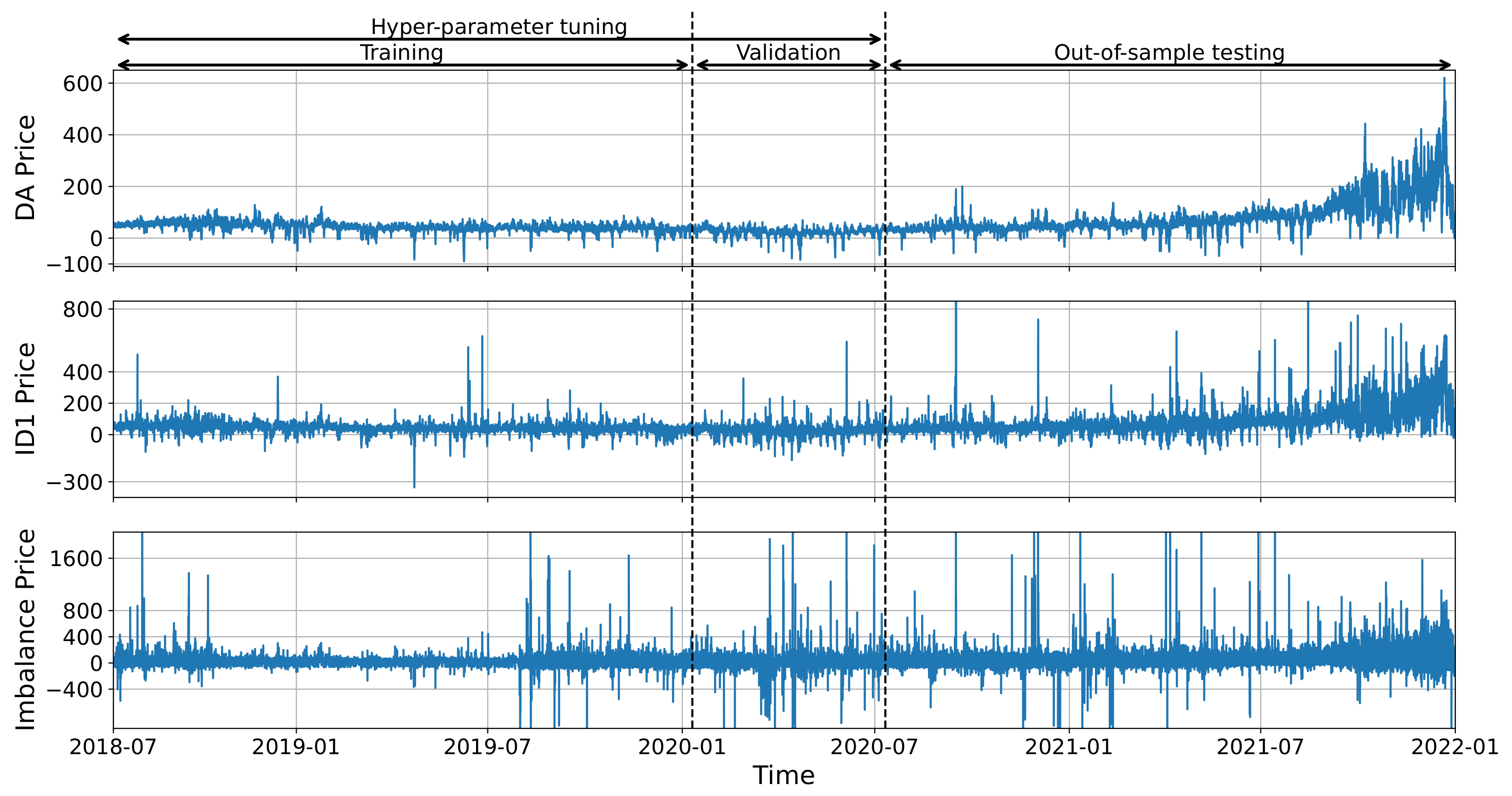
Figure 2 presents the time series of three electricity prices: the DA price, the quarterly ID${}_1$ price, and the imbalance price.

The plots show clearly that the imbalance price is much more volatile than the prices in the quarterly IC market or in the DA market. Moreover, in the considered time-frame, the imbalance price exhibited many positive and negative extreme spikes, with a minimum of around $-6500$ EUR/MWh and a maximum of around 24,500 EUR/MWh (for better clarity of Figure 2, we do not show the extremes in the plot). Such values are impossible to reach in the DA (a min of $-500$ and a max of 3000) and IC (a min of $-9999$ and a max of 9999) markets. Therefore, the participation in the balancing market comes with a high risk for a BRP. 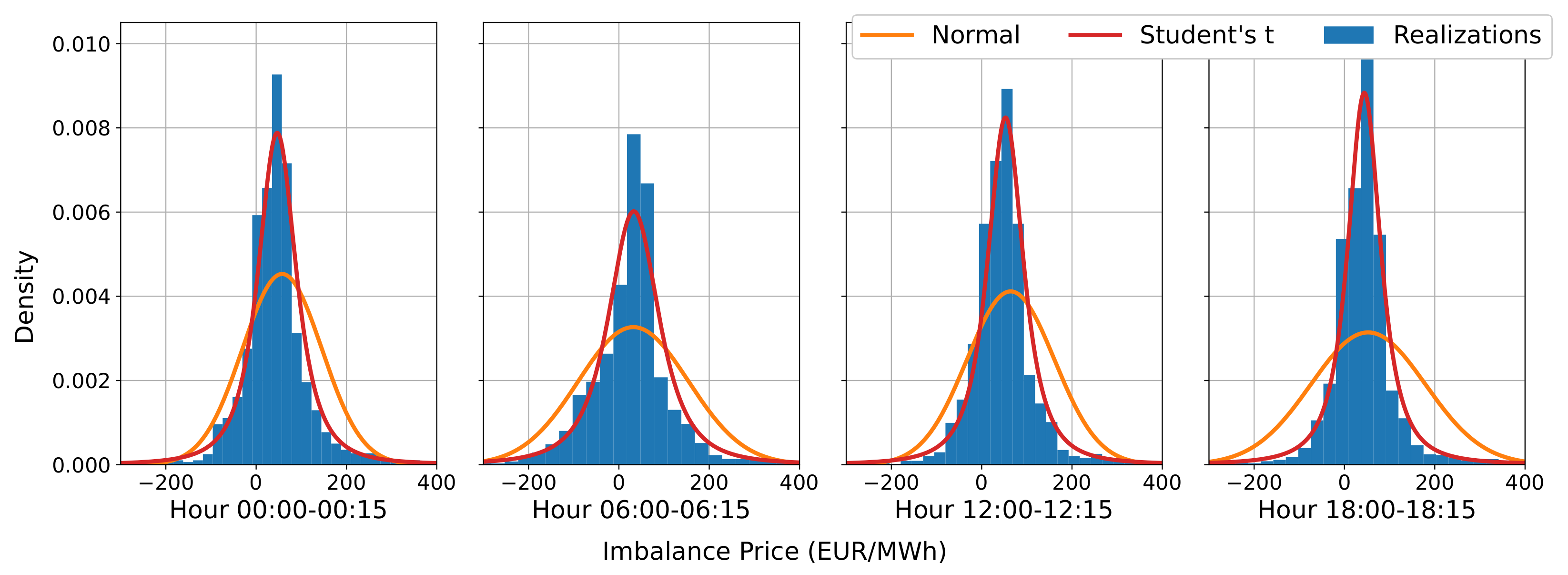This confirms Figure 3, which shows histograms of imbalance prices for selected hours (the range of prices was limited for better clarity of the histograms).

The fitted densities prove that the data are heavy-tailed as the three-parametric Student’s t distribution $t(\mu ,\sigma ,\tau )$ seems to fit the data much better than the normal distribution $\mathcal{N}(\mu ,{\sigma }^2)$. The two mentioned distributions will be later utilized in the application study. All the distributions belong to the location-scale family with $\mu$, $\sigma$, and $\tau$ being the location, scale, and tail-weight (degrees of freedom) parameters, respectively.

2.3. Data

The data utilized in the study are collected from four different sources. The spot market data (DA, IA and IC transactions and prices) from the EEX transparency, the day-ahead forecast data (load and renewable generation) from the ENTSO-E transparency, the balancing market data (imbalance price, imbalance volume, aFRR and mFRR capacity and energy market data) from the regelleistung.net and the fuels and emission allowance prices from the ICE. The complete dataset contains observations between 12 July 2018 and 31 December 2021 as the aFRR and mFRR data are not available for the preceding time. We cleaned the data from missing values using the R package tsrobprep [43].

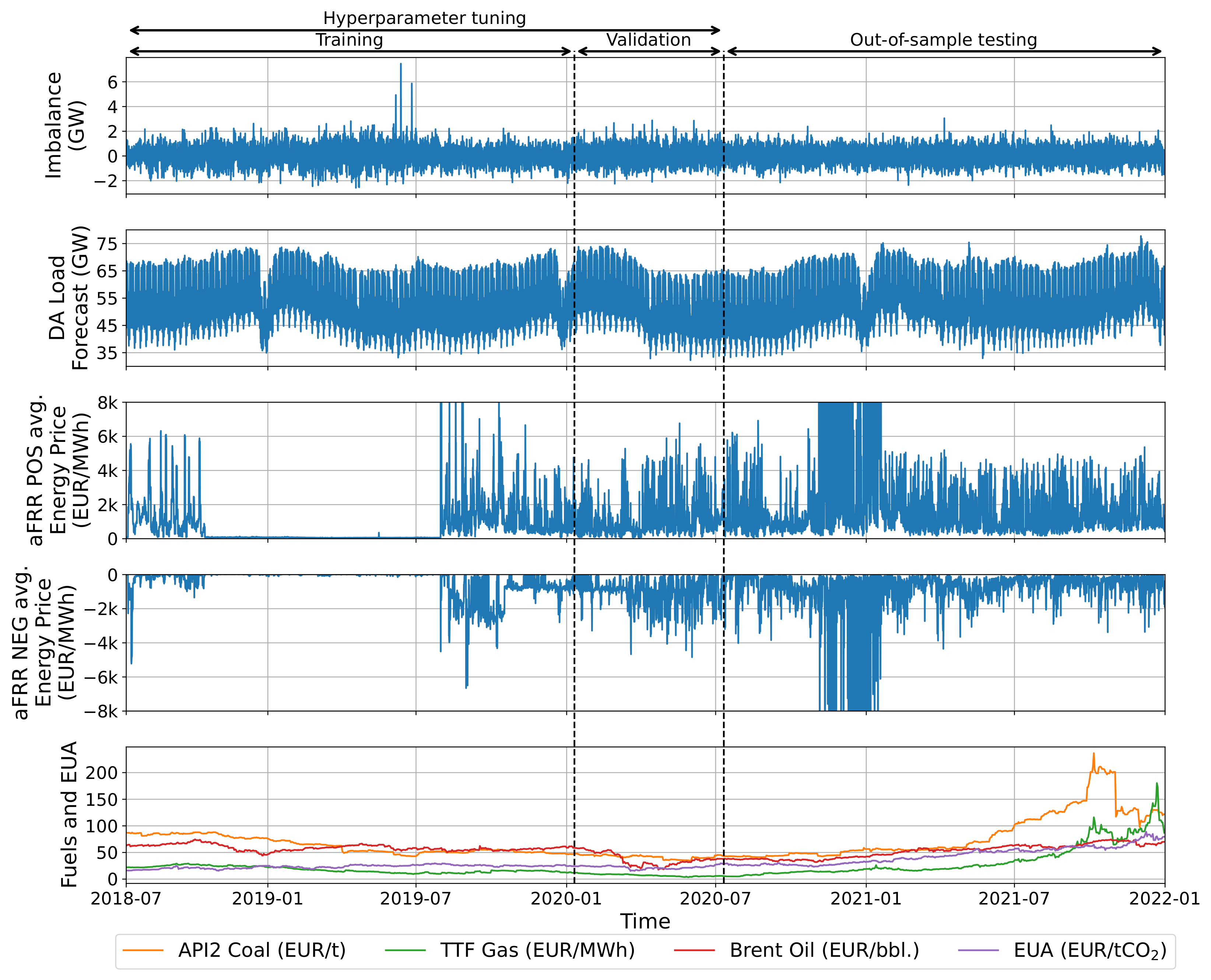
Figure 4 presents time series plots of selected external regressors and is a complement to Figure 2.

In both figures, we marked the initial in-sample, the hyperparameter tuning, and the out-of-sample periods. Let us note the structural break in the aFRR positive and negative average energy prices between October 2018 and July 2019. During this period, the mixed-pricing method was used in the tendering of aFRR and mFRR, i.e., both capacity and energy prices were used to select the cheapest BSPs. However, this method was abolished following a decision by the Düsseldorf Higher Regional Court due to an appeal and the capacity pricing (as described in Section 2.1) was immediately re-introduced.

3. Models and Estimation

This section describes the input features and the models that use them to forecast the imbalance price ${\mathrm{IP}}^{d,qh}$. In the EPF literature, it is typical to use autoregressive effects of the modelled prices; here, however, we cannot do it as the German imbalance prices are published once a month. For the price calculation in the IC market, we use the ${}_x{\mathrm{ID}}_y$ definition of Narajewski and Ziel [26]. Let us recall that the ${}_x{\mathrm{ID}}_y$ is a volume-weighted average price of all transactions in the IC market that take place in the $[x+y,x)$ time interval prior the delivery. The x parameter defines the time to delivery of the measured window and the y parameter the window length. For example, the EPEX ID${}_3$, which measures the price based on all transactions between 3 h and 30 min prior the delivery, is denoted as ${}_{0.5}{\mathrm{ID}}_{2.5}$ in terms of ${}_x{\mathrm{ID}}_y$.

3.1. Input Features

The following features are considered in the exercise of modelling the imbalance price ${\mathrm{IP}}^{d,qh}$ for day d and quarter-hour $qh$ with $qh=1,\dots ,96$. Whenever mentioning the corresponding product, we mean the same delivery hour, e.g., for $qh=6$, the corresponding hourly delivery time is 01:00 and quarter-hourly is 01:15. Note that we utilize only the information available until 30 min before the delivery.

• Corresponding EPEX price indices: DA${}^{d,h}$, IA${}^{d,qh}$, ID${}_1^{d,i}$, ID${}_3^{d,i}$, and ID-Index${}^{d,i}$ for $i=h,qh$ (8 regressors) (The ID-Index is a volume-weighted average price of all corresponding ID transactions);
• Most recent 15-minute intraday prices ${}_x{\mathrm{ID}}_{15\min }^{d,h}$ for $h=1,\dots ,24$ and ${}_x{\mathrm{ID}}_{15\min }^{d,qh}$ for $qh=1,\dots ,96$ ($24+96=120$ regressors);
• Corresponding intraday price differences $\Delta {}_x^{}{\mathrm{ID}}_{5\min }^{d,qh}={}_x^{}{\mathrm{ID}}_{5\min }^{d,qh}-{}_{x+5\min }^{}{\mathrm{ID}}_{5\min }^{d,qh}$ with $x=30,35,\dots ,55$ min (6 regressors);
• DA forecasts of load, wind onshore, wind offshore and solar generation: ${\mathrm{Load}}^{d,qh}$, ${\mathrm{WiOn}}^{d,qh}$, ${\mathrm{WiOff}}^{d,qh}$, ${\mathrm{Solar}}^{d,qh}$ for $qh=1,\dots ,96$ ($96\times 4=384$ regressors);
• DA forecasts mentioned above for the previous day: ${\mathrm{Load}}^{d-1,qh}$, ${\mathrm{WiOn}}^{d-1,qh}$, ${\mathrm{WiOff}}^{d-1,qh}$, ${\mathrm{Solar}}^{d-1,qh}$ for $qh=1,\dots ,96$ ($96\times 4=384$ regressors);
• Most recent available estimation (which is provided by the TSOs around 15 min after delivery) of the imbalance volumes ${\mathrm{Imb}}^{d,qh-i}$ for $i=4,\dots ,7$ (4 regressors);
• aFRR prices: ${\mathrm{aFRR}}_{i,j,k}^{d,qh}$ for $i=\mathrm{POS},\mathrm{NEG}$ indicating the positive or negative balancing side, $j=\mathrm{CAP},\mathrm{EN}$ indicating the capacity or energy price, and $k=\min ,\mathrm{avg},\max$ indicating the minimum, average or maximum price ($6\times 2$ regressors);
• mFRR prices: ${\mathrm{mFRR}}_{i,j,k}^{d,qh}$ with $i,j,k$ as above ($6\times 2$ regressors);
• Previous day coal, gas, oil and EUA prices: ${\mathrm{Coal}}^{d-1}$, ${\mathrm{Gas}}^{d-1}$, ${\mathrm{Oil}}^{d-1}$, ${\mathrm{EUA}}^{d-1}$ (4 regressors);
• Weekday dummies ${\mathrm{DoW}}_i^d$ for $i=1,\dots ,7$ (7 regressors);
• Cubic periodic B-splines $S_i^d$ for $i=1,\dots ,6$ constructed as in Ziel et al. [44] (6 regressors).

In total, we consider 948 regressors for the modelling exercise. Let us shortly motivate the choice of these particular variables. Previous studies [26,29] have shown that the past prices can bring a lot of information regarding the future intraday price level and distribution. We expect similar behaviour in the imbalance price development, and thus we consider the price data, especially the most recent intraday prices and price differences. Similarly, the DA forecasts of fundamental variables might help in explaining the expected volatility. Naturally, the most recent intraday forecasts would be much more informative, but unfortunately these data are not publicly available and very expensive to obtain. The most recent observed imbalance values might indicate the expected imbalance in the considered quarter-hour. The aFRR and mFRR prices are natural regressors for the imbalance prices, as they directly contribute to their values. The fuel and EUA prices should explain the general price trend, and finally the weekday dummies and cubic B-splines account for weekly and annual seasonality, respectively.

3.2. Naive

Following the research on intraday markets [26,28,29,30] where the authors find the most recent intraday price to be a very good and simple model, we construct the naive model in a similar manner. That is to say, we assume the expected imbalance price to be equal the observed quarter-hourly ID${}_1$ price

$$\mathbb{E}\left({\mathrm{IP}}^{d,qh}\right)={\mathrm{ID}}_1^{d,qh}.$$

(2)

To obtain a distribution of imbalance prices, we use additionally the bootstrap method [45] which was successfully applied in previous EPF research studies [18,29,36,46]. The in-sample bootstrapped errors are added to the forecasted expected price to derive the distribution forecast

$${\widehat{\mathrm{IP}}}_m^{D+1,qh}=\widehat{\mathbb{E}\left({\mathrm{IP}}^{D+1,qh}\right)}+{\widehat{\epsilon }}_m^{D+1,qh}\mathrm{for}m=1,\dots ,M$$

(3)

where ${\widehat{\epsilon }}_m^{D+1,qh}$ are drawn with replacement in-sample residuals for day $D+1$, i.e., we sample from the set of ${\widehat{\epsilon }}^{d,qh}={\mathrm{IP}}^{d,qh}-{\widehat{\mathrm{IP}}}^{d,qh}$ for $d=1,\dots ,D$.

3.3. Lasso with Bootstrap

The lasso regression of Tibshirani [47] is a very simple and powerful tool for linear model estimation, and thus gained high popularity and reputation in the EPF literature [19,20,24,25,26,30]. It serves both model estimation and variable selection, and therefore for the model we use all the regressors described in Section 3.1, and we denote such vector as ${\mathit{X}}^{d,qh}$. The formula for the model is

$${\mathrm{IP}}^{d,qh}={\mathit{X}}^{d,qh}{\mathit{\beta }}^{qh}+{\epsilon }^{d,qh}$$

(4)

and the lasso estimator is given by

$${\widehat{\mathit{\beta }}}^{qh}=arg\underset{{\mathit{\beta }}^{qh}}{min}\left\{{\left|\left|{\mathrm{IP}}^{d,qh}-{\mathit{X}}^{d,qh}{\mathit{\beta }}^{qh}\right|\right|}_2^2+\lambda \left|\right|{\mathit{\beta }}^{qh}{\left|\right|}_1\right\}$$

(5)

where $\lambda$ is a tuning parameter. The lasso estimator expects scaled inputs, and, in addition to that, we apply on the inputs the variance stabilizing asinh transformation as suggested by Uniejewski et al. [48] with the inverse proposed by Narajewski and Ziel [26]. The $\lambda$ parameter is tuned based on a Bayesian information criterion (BIC) for $\lambda \in \mathsf{\Lambda }=\{{\lambda }_i=2^i|i\in \mathcal{G}\}$, where $\mathcal{G}$ is an equidistant grid from $-15$ to 1 of length 50, similarly as in the paper of Narajewski and Ziel [26]. Let us note that similarly as for the naive, the lasso model estimates the expected imbalance price and, to obtain a distribution forecast, we need the bootstrap procedure described in Equation (3).

3.4. Gamlss with Lasso

The gamlss framework of Rigby and Stasinopoulos [49] is an extension of the generalized additive models by allowing to build explicit additive models not only for the location, but also scale and shape parameters of a given distribution. Its potential was already noticed in the EPF literature [29,34]; however, it has not yet gained such popularity as the lasso estimation. For the regressor input vector ${\mathit{X}}^{d,qh}$, we have the following model:

$$g_i\left({\theta }_i^{d,qh}\right)={\mathit{X}}^{d,qh}{\mathit{\beta }}_i^{qh}$$

(6)

with $g_i$ being the link function, and ${\theta }_i^{d,qh}\in {\Theta }^{d,qh}$ the parameters of the distribution given by the cumulative distribution function $F(x;{\theta }^{d,qh})$. ${\Theta }^{d,qh}$ denotes a distribution parameter space. In the study, we consider the normal and t distributions. The link function for the location parameter is the identity function $g_1\left(x\right)=x$, and, for the scale and tail-weight, the softplus function $g_2\left(x\right)=log(exp\left(x\right)+1)$. The link functions are shown in Figure 5.

The model in Equation (6) is actually a glmlss one as we consider only linear effects of the inputs. Moreover, the size of ${\mathit{X}}^{d,qh}$ could make the optimizing algorithm converge very slowly, especially for the 3-parametric distribution. Therefore, we additionally use the lasso regularization (5) as described e.g., by Ziel [50]; however, we do not directly use the gamlss [51] and gamlss.lasso [52] R packages as their deterministic algorithm has issues with convergence due to the very heavy tails of our data. Instead, we utilize the TensorFlow [53] and Keras [54] framework by building a simple neural network with a single linear hidden layer and given probability distribution as output. For each of the distribution parameters, we use different regularization parameter ${\lambda }_i\in \left({10}^{-5},10\right)$. We also allow for no regularization of each of the distribution parameters. The model is estimated by maximizing the log-likelihood using the Adam algorithm. The learning rate is assumed to be in the interval $({10}^{-5},{10}^{-1})$, and we tune all the parameters using the Optuna [55] package in Python with the number of iterations arbitrarily set to 500. Depending on distribution, we have 5 or 7 hyperparameters to tune. Let us note that the input vector ${\mathit{X}}^{d,qh}$ is standardized prior to the modelling.

3.5. Probabilistic Neural Networks

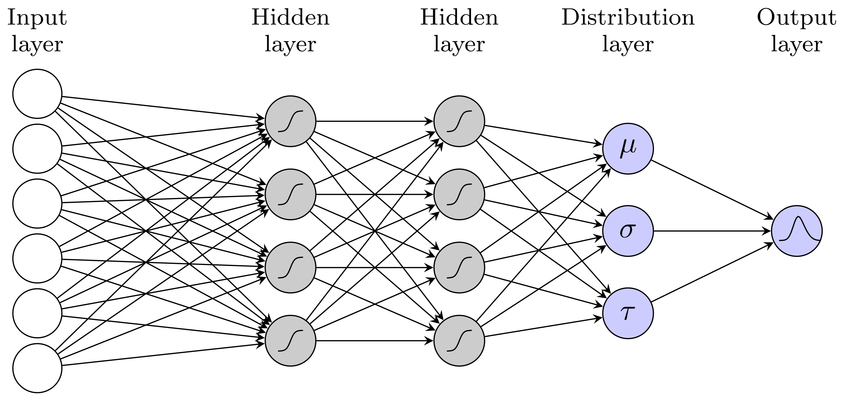
The probabilistic neural network model is simply a multilayer perceptron (MLP) that models distribution parameters instead of price values, as shown in Figure 6. Let us note that, if we remove the hidden layers, we obtain the gamlss model described in the previous section.

The approach of probabilistic MLP in EPF was first introduced by Marcjasz et al. [46] for the day-ahead prices. For mathematical details, see the aforementioned manuscript. The considered model assumes two or three hidden layers and outputs normal or t distribution. For the distribution parameters, we use the same link functions as in Figure 5. We regularize the model through input feature selection, $L_1$ regularization of the hidden layers and their weights, and a dropout layer. We tune them together with the number of hidden layers, their activation functions, number of neurons and the learning rate. In the following, we present a list of all hyperparameters considered in the tuning:

• Input feature selection as described in Section 3.1 (20 hyperparameters);
• Dropout layer—whether to use the dropout layer after the input layer, and if yes at what rate. The rate parameter is drawn from $(0,1)$ interval (up to 2 hyperparameters);
• Size of the network—either two or three hidden layers (1 hyperparameter);
• Activation functions in the hidden layers. The possible functions are: elu, relu, sigmoid, softmax, softplus, and tanh (1 hyperparameter per layer);
• Number of neurons in the hidden layers. The values are drawn from $[24,1024]$ interval (1 hyperparameter per layer);
• $L_1$ regularization–whether to use the $L_1$ regularization on the hidden layers and their weights and if yes at what rate. The rate is drawn from $({10}^{-5},10)$ interval (up to four hyperparameters per layer);
• Learning rate for the Adam algorithm drawn from $({10}^{-5},{10}^{-1})$ interval (one hyperparameter).

In total, we have up to 42 hyperparameters to tune. The selected input features are normalized prior to the model estimation. Similarly as for the gamlss model, we use the Tensorflow [53] and Keras [54] framework for model estimation, and the Optuna [55] for hyperparameter tuning with the number of iterations arbitrarily set to 1000. The model contains additionally some elements which are not subjects of the tuning exercise. These are size of the learning and validation sets, the optimizing algorithm, the number of epochs fixed to 1500, and batch size fixed to 32. We estimate the model by maximizing the log-likelihood, and we use the early stopping callback with the patience of 50 epochs.

4. Application Study

4.1. Setting

Due to the high complexity of the models and the need for comprehensive and computational heavy hyperparameter tuning, we consider in the study only selected quarter-hours. That is to say, we use all quarter-hours of representative hours 0, 6, 12, and 18, i.e., $qh\in QH=\{1,2,3,4,25,26,27,28,49,50,51,52,73,74,75,76\}$. As described in Section 3, for each $qh$, we build separate models, including a separate hyperparameter tuning. Thus, we reduce the number of them from 96 to 16 without loss of generality.

The forecasting study utilizes a rolling window scheme with $D=730$ days in-sample and $N=539$ days out-of-sample. In case of gamlss and probabilistic MLP models, the in-sample period is split to 547 days used for training and 183 for validation. To forecast prices on each of the out-of-sample days $d=1,\dots ,N$, we fit the data to the D recent in-sample days. Then, after obtaining the forecast, we roll the window forward by one day and repeat the procedure until the end of the out-of-sample set. The hyperparameter tuning is performed once, using the initial in-sample data, as shown in Figure 2 and Figure 4. We aim for a very short-term forecasting utilizing the information available up to 30 min before the delivery. The naive and lasso models forecast the imbalance price distribution through $M=$ 10,000 bootstrap samples, whereas the gamlss and probabilistic ANN models forecast directly the assumed distribution.

4.2. Evaluation

Following the conclusions of Gneiting and Raftery [56], our main evaluation measure is the continuous ranked probability score (CRPS) as it is a strictly proper scoring rule for marginal distribution forecasts. Additionally, we calculate the values of the RMSE, MAE and empirical coverage as supplementary measures. For statistically significant conclusions, we conduct the Diebold and Mariano [57] test using the respective CRPS losses. In this subsection, we provide details regarding the calculation of the mentioned measures.

The CRPS is approximated using the pinball loss

$${\mathrm{CRPS}}^{d,qh}=\frac{1}{R}\sum _{\tau \in r}{\mathrm{PB}}_{\tau }^{d,qh}$$

(7)

for a dense equidistant grid of probabilities r between 0 and 1 of size R, see e.g., Nowotarski and Weron [18]. In our study, we consider $r=\{0.01,0.02,\dots ,0.99\}$ of size $R=99$. ${\mathrm{PB}}_{\tau }^{d,qh}$ is the pinball loss with respect to probability $\tau$. Its formula is given by

$${\mathrm{PB}}_{\tau }^{d,qh}=\left(\tau -{\mathbb{1}}_{\left\{{\mathrm{IP}}^{d,qh}<{\widehat{Q}}_{\tau }^{d,qh}\right\}}\right)\left({\mathrm{IP}}^{d,qh}-{\widehat{Q}}_{\tau }^{d,qh}\right)$$

(8)

where ${\widehat{Q}}_{\tau }^{d,qh}$ is a forecast of $\tau$-th quantile of ${\mathrm{IP}}^{d,qh}$ price. To calculate the overall CRPS value, we use a simple average

$$\mathrm{CRPS}=\frac{1}{16N}\sum _{qh\in QH}\sum _{d=1}^N{\mathrm{CRPS}}^{d,qh}.$$

(9)

The formulas for the supplementary measures are given by

$$\tau \%\text{-}\mathrm{cov}=\frac{1}{16N}\sum _{qh\in QH}\sum _{d=1}^N{\mathbb{1}}_{\left\{{\widehat{Q}}_{(1-\tau )/2}^{d,qh}<{\mathrm{IP}}^{d,qh}<{\widehat{Q}}_{(1+\tau )/2}^{d,qh}\right\}},$$

(10)

$$\mathrm{RMSE}=\sqrt{\frac{1}{16N}\sum _{qh\in QH}\sum _{d=1}^N{\left({\mathrm{IP}}^{d,qh}-{\widehat{\mu }}^{d,qh}\right)}^2}$$

(11)

and

$$\mathrm{MAE}=\frac{1}{16N}\sum _{qh\in QH}\sum _{d=1}^N\left|{\mathrm{IP}}^{d,qh}-{\widehat{Q}}_{0.5}^{d,qh}\right|$$

(12)

where $\tau \in \{0.5,0.9,0.98\}$, and ${\widehat{\mu }}^{d,qh}$ is a forecast of expected ${\mathrm{IP}}^{d,qh}$ price.

The DM test measures the statistical significance of the difference between the accuracy of the forecasts of model A and model B, and it is commonly used in the EPF literature [20,25,26,29]. Denote $L_Z^d={\left(L_Z^{d,qh}\right)}_{qh\in QH}^{\prime }$ the vector of out-of-sample losses for day d of model Z. Formally, we choose $L_Z^{d,qh}={\mathrm{CRPS}}^{d,qh}$. The multivariate loss differential series

$${\Delta }_{A,B}^d=\left|\right|L_A^d{\left|\right|}_1-\left|\right|L_B^d{\left|\right|}_1$$

(13)

defines the difference of losses in $\left|\right|·{\left|\right|}_1$ norm. For each pair of models, we compute the p-value of two one-sided DM tests. The first one is with the null hypothesis ${\mathcal{H}}_0:\mathbb{E}\left({\Delta }_{A,B}^d\right)\le 0$—that is to say, the outperformance of the forecasts of model B by the ones of model A. The second test is with the reverse null hypothesis ${\mathcal{H}}_0:\mathbb{E}\left({\Delta }_{A,B}^d\right)\ge 0$, and it complements the former one.

4.3. Results

Table 1. Error measures of the considered models. Colour indicates the performance columnwise (the greener, the better). With bold, we depicted the best values in each column.

	CRPS	MAE	RMSE	50%-Cov	90%-Cov	98%-Cov
Naive	23.04	61.22	115.2	0.2847	0.8011	0.9525
Lasso	24.91	65.06	124.5	0.2784	0.7825	0.9417
gamlss.N	36.09	88.70	154.5	0.3294	0.6158	0.7067
gamlss.t	24.24	65.70	124.2	0.4074	0.8851	0.9739
probNN.N	35.67	92.84	368.5	0.5037	0.8460	0.9249
probNN.t	25.85	68.74	129.2	0.3912	0.8733	0.9645
Combination	22.94	62.84	117.8	0.3480	0.8749	0.9787

presents the results of the forecasting study. We see that the lowest error values are obtained for the naive model which forecasts the imbalance price simply with the quarterly ID${}_1$ price. However, its empirical coverage is very bad. The second-lowest errors are produced by the gamlss model that assumes the t-distribution, and this model provides the best values in terms of 90% and 98% empirical coverage. The generalization from gamlss to probabilistic neural network model does not bring any improvement for the t-distribution. Based on the performance of the two mentioned models, we decided to try a simple forecast combination by averaging the forecasts of the two models. In the probabilistic case, it means to average the cumulative distribution functions. However, as the naive one is not available, instead we sample from both distributions an equal number of observations. This way, we can derive the statistics necessary for the evaluation. This brings a small improvement in the CRPS and in the coverage, compared to the naive model. Let us also mention very high errors of the models that assume the normal distribution. This is inline with the previous studies [29] on intraday price development, and it was expected based on Figure 2 and Figure 3. Interestingly, the probNN.N model provides a very accurate 50% coverage, but not as good 90% or 98% coverages. Finally, the lasso model performs slightly worse than the naive in all terms, which indicates that one cannot gain any improvement only with linear terms.

Figure 7 shows the pinball score values over quantiles $\tau \in r$ and the ratio to the naive model. For better clarity, we removed from the right plot the models assuming normal distribution. We see that the models have generally more issues with forecasting the right tail of the distribution. Interestingly, the lasso model forecasts the quantiles up to around 0.3 slightly better than the naive; however, it loses very much in the higher quantiles. In addition, the combination of naive and gamlss.t is slightly better than the naive in both tails, however not that good in the central part of the distribution. This shows that a forecast combination, as e.g., in Berrisch and Ziel [58], could likely improve the overall score. Figure 8 presents the CRPS values over considered quarter-hours. The naive model seems to be the best across all quarter-hours except for two at hour 6. There, the gamlss.t is slightly better than the naive; however, the difference is not large and probably not significant. Again, some additional improvement comes as a result of combining the naive with the gamlss.t model.

Finally, Figure 9 provides p-values of the DM test obtained using CRPS loss. This figure only confirms the conclusions that we made based on Table 1. Namely, the forecasts of the naive model are significantly the best among considered models and the ones of gamlss.t model the second-best. Moreover, the combination of naive and gamlss.t is not significantly different to the naive itself.

5. Conclusions

The paper raised the novel issue of probabilistic imbalance electricity price forecasting in the German market. The participation in balancing is mandatory for every market player, and therefore this subject is crucial for them. The analysis assumed a setting of a very short-term forecasting, 30 min before the physical delivery. We considered various state-of-art methods for probabilistic EPF; however, none of them could provide better forecasts in terms of CRPS, MAE, and RMSE than the naive ID${}_1$ price. On the other hand, the gamlss and probabilistic neural networks models provide forecasts with far higher empirical coverage than the naive. This is evidence that the results might be improved, e.g., using intraday power generation forecasts or forecasting combination methods, e.g., [58].

This paper contributes both to the broad EPF and to the scarce electricity balancing literature by raising an important topic and drawing researchers’ attention to the imbalance market. It also contributes to the electricity trading literature, as the imbalance price is a component that strongly influences the total cashflow of electricity traders. The key limitation of this paper is the unavailability of the intraday-updated forecasts which could improve the forecasting performance. Other limitations are the constantly changing conditions and regulations of the German balancing market, which makes it harder for the models to find any pattern in price development.

The obtained results are an argument towards the market efficiency between the intraday and balancing markets. This extends the conclusions of the intraday market being close to market efficiency [26,30]. Therefore, given the difficulty in forecasting the imbalance prices and the potential size of forecasting errors, the BRPs should minimize their imbalance rather than seeking opportunities in the balancing market. Therefore, electricity portfolio managers and traders should bear this in mind when writing their algorithmic trading strategies or solving their intraday imbalance positions.

The relevancy and scarce literature on the topic of probabilistic imbalance price forecasting results in a big potential for future research. Possible directions are trading strategies based on intraday and imbalance price forecasts, improving the models by incorporating the intraday-updated forecasts or advanced expert aggregation techniques for probabilistic forecast combination. Another direction is considering other markets of similar structure, where such study could bring much better results, especially in less liquid markets.