
Bidding a Battery on Electricity Markets and Minimizing Battery Aging Costs: A Reinforcement Learning Approach

 ,
,  ,
,  and
and
Abstract
:1. Introduction
2. Literature Review
2.1. Financial Exploitation of Battery Storage
2.2. Reinforcement Learning Applications for Batteries
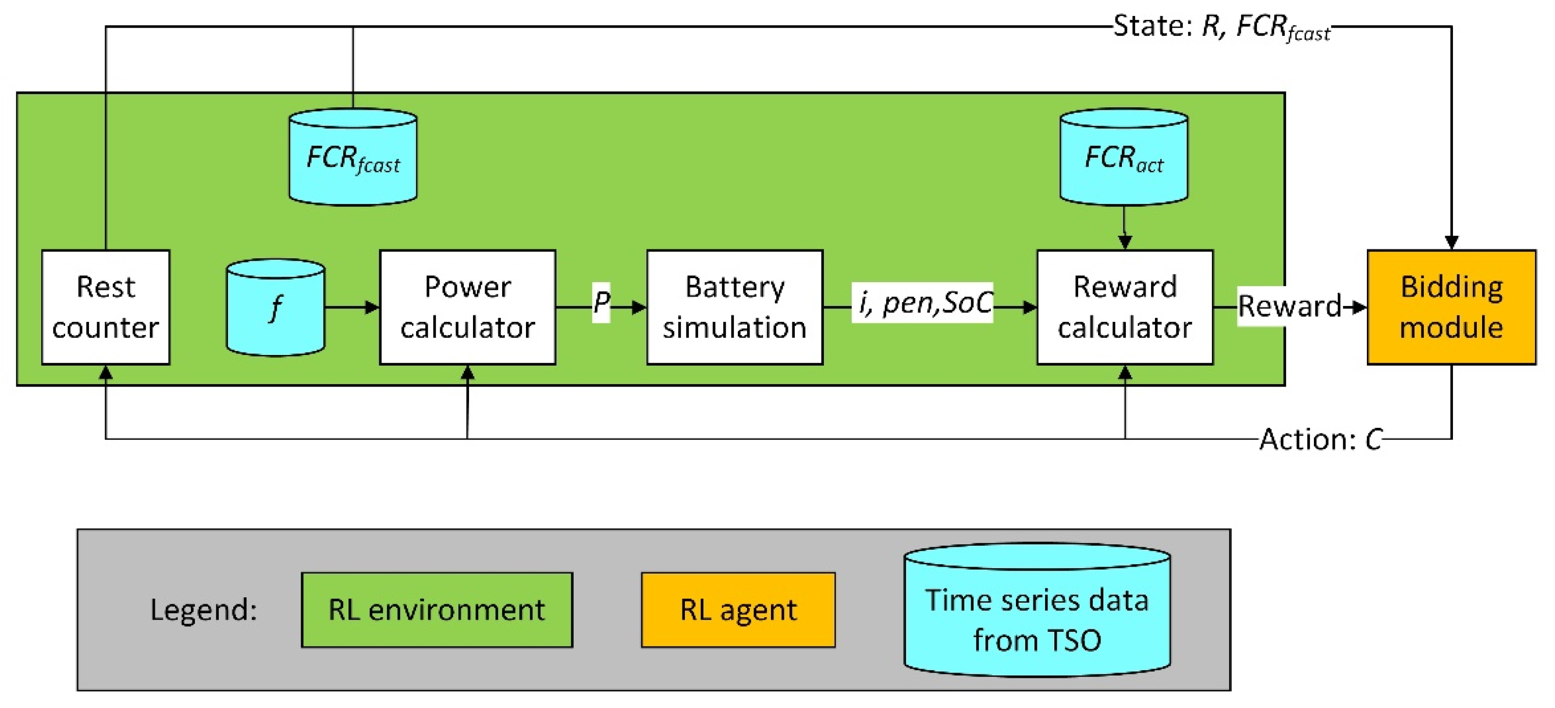
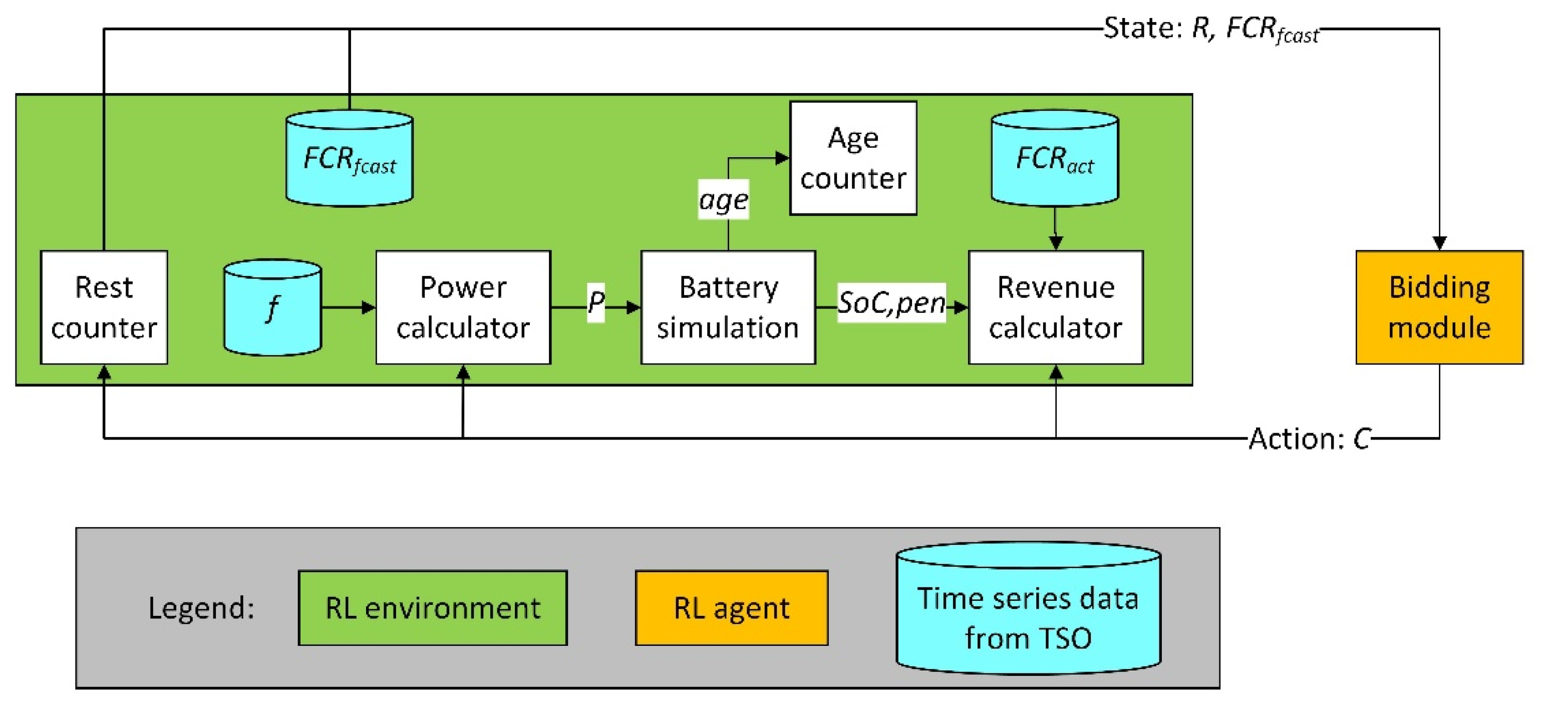
3. Methodology
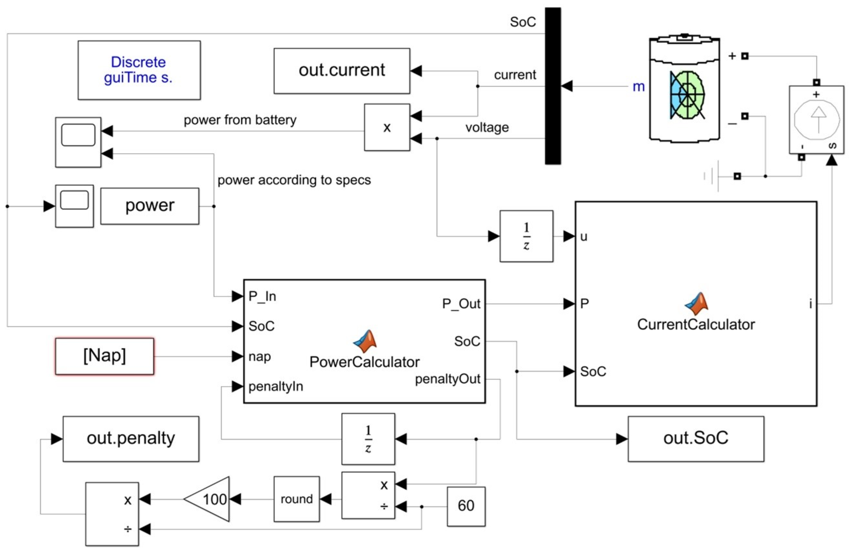
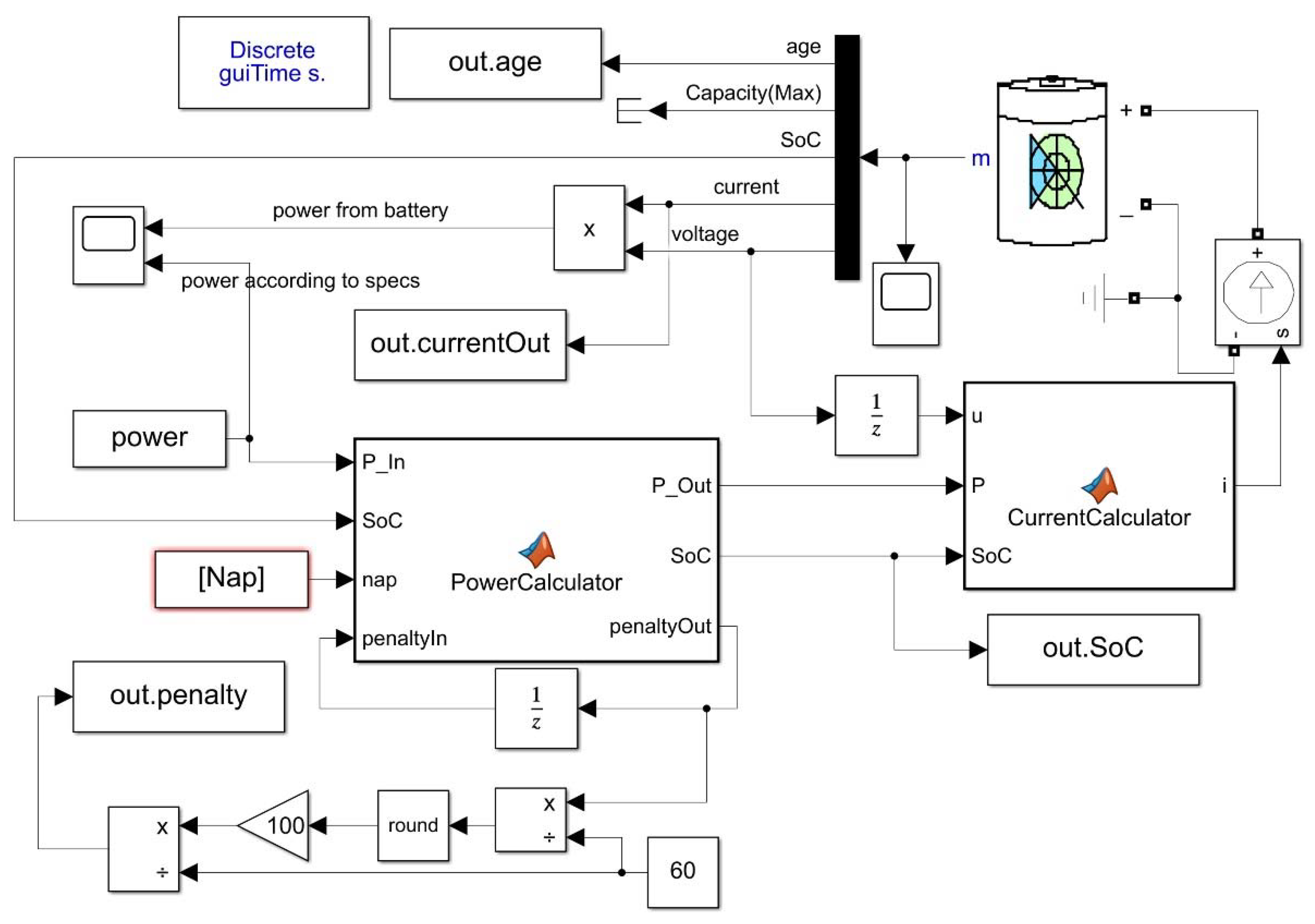
4. Implementation
5. Results
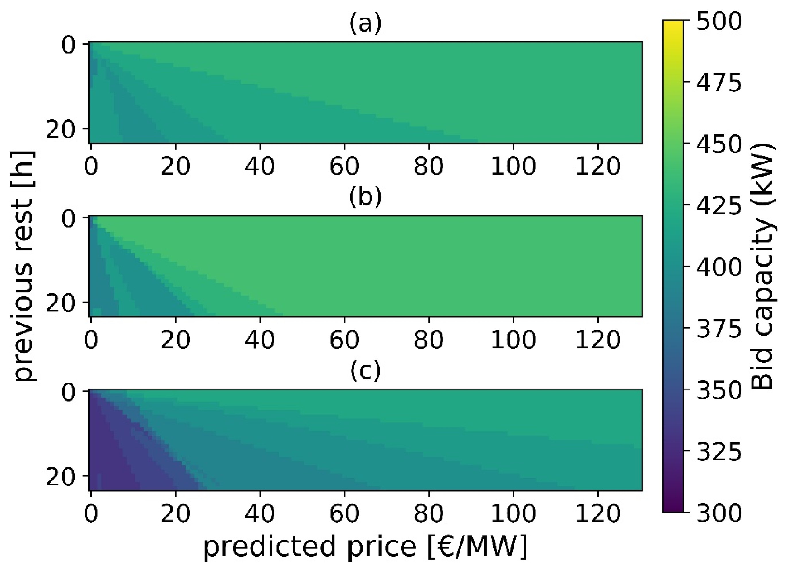
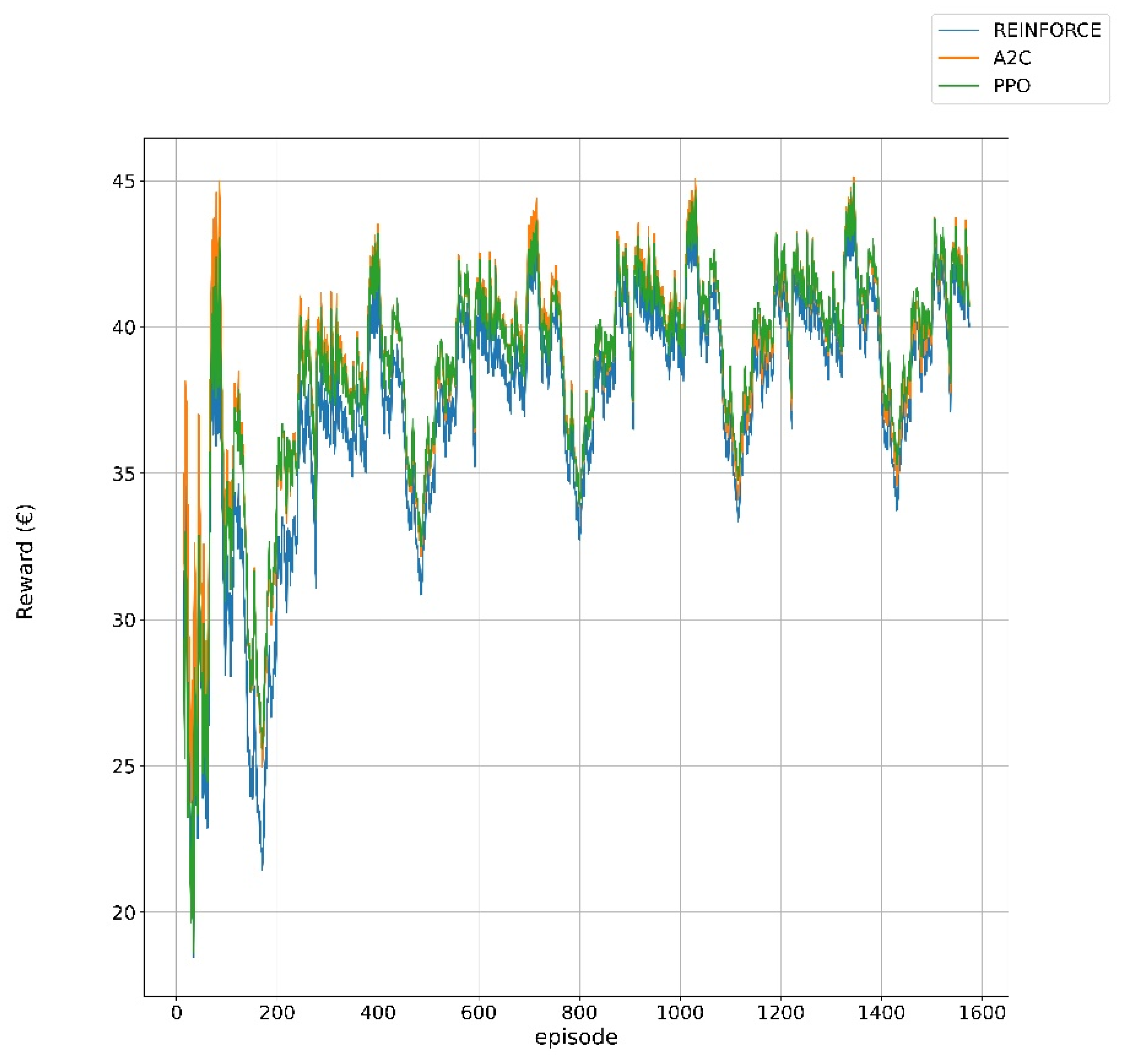
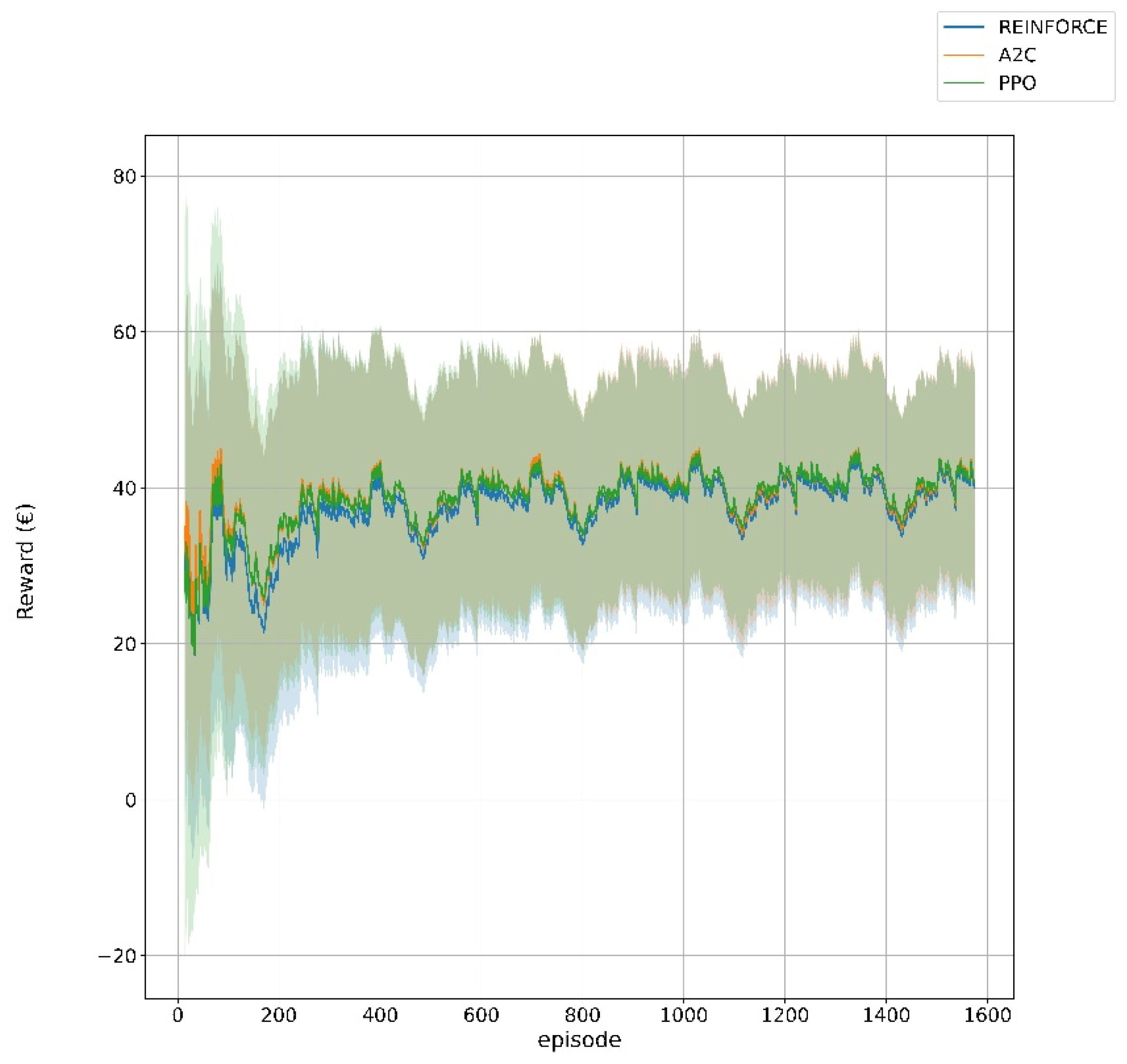
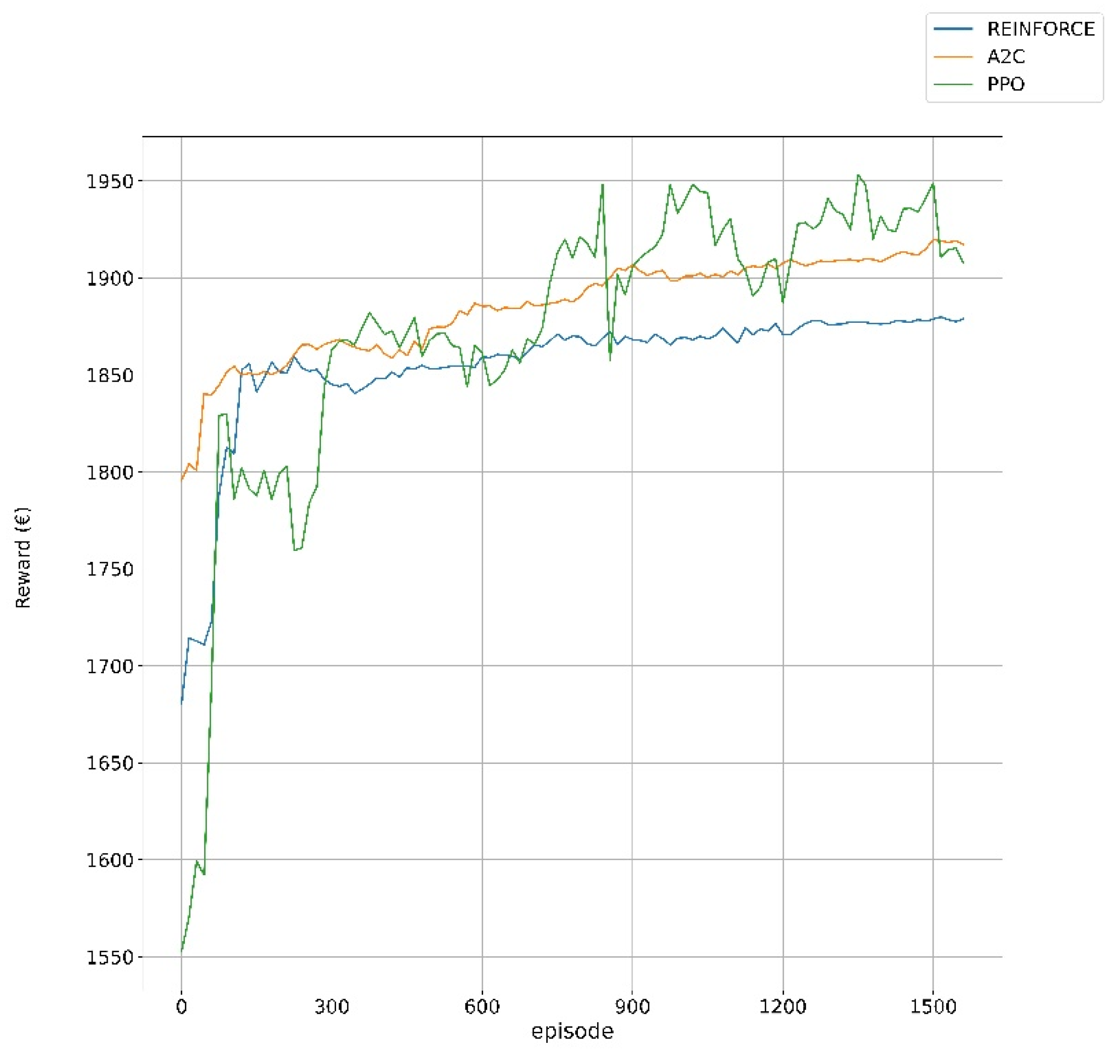
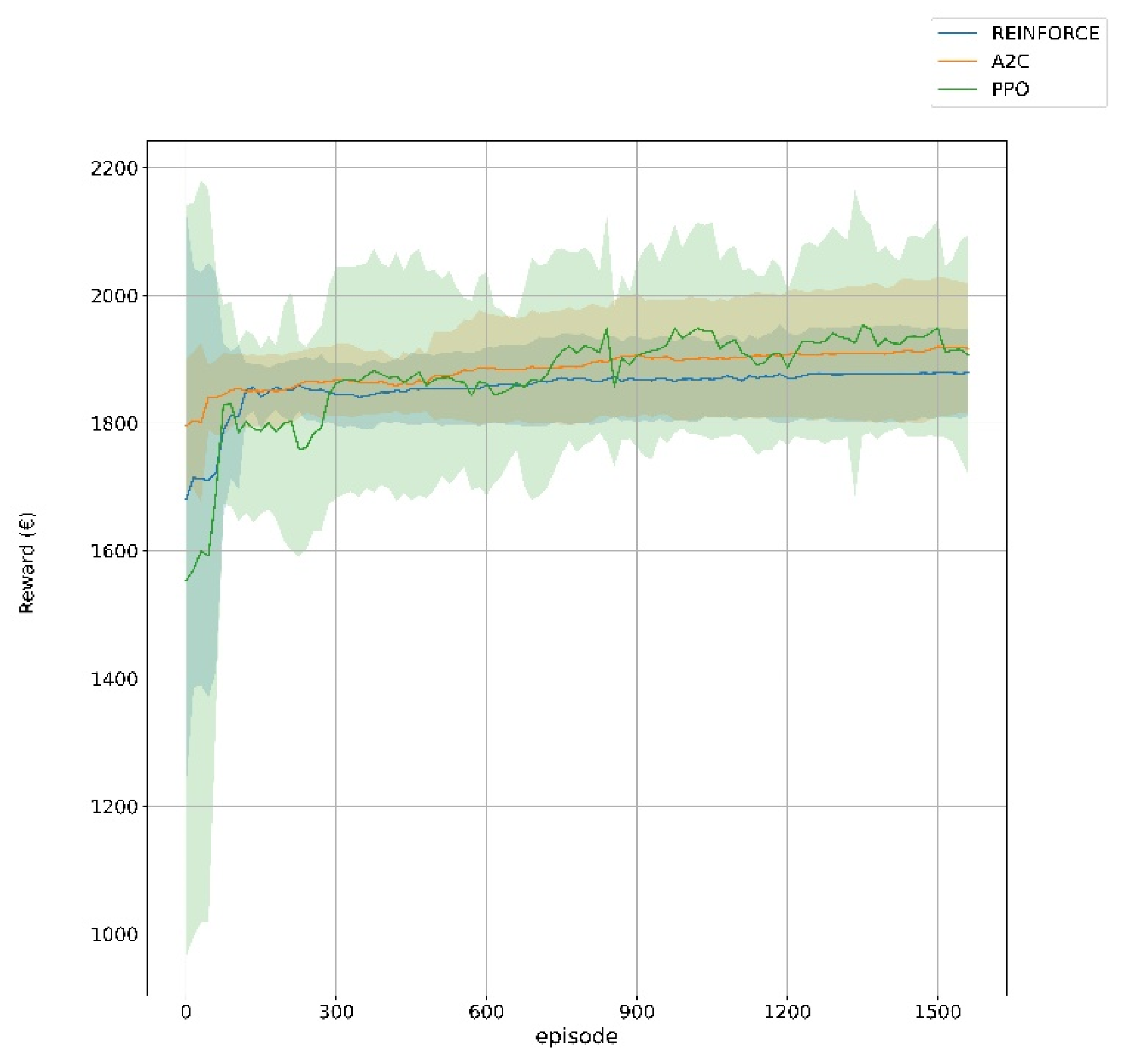
5.1. Training and Validation
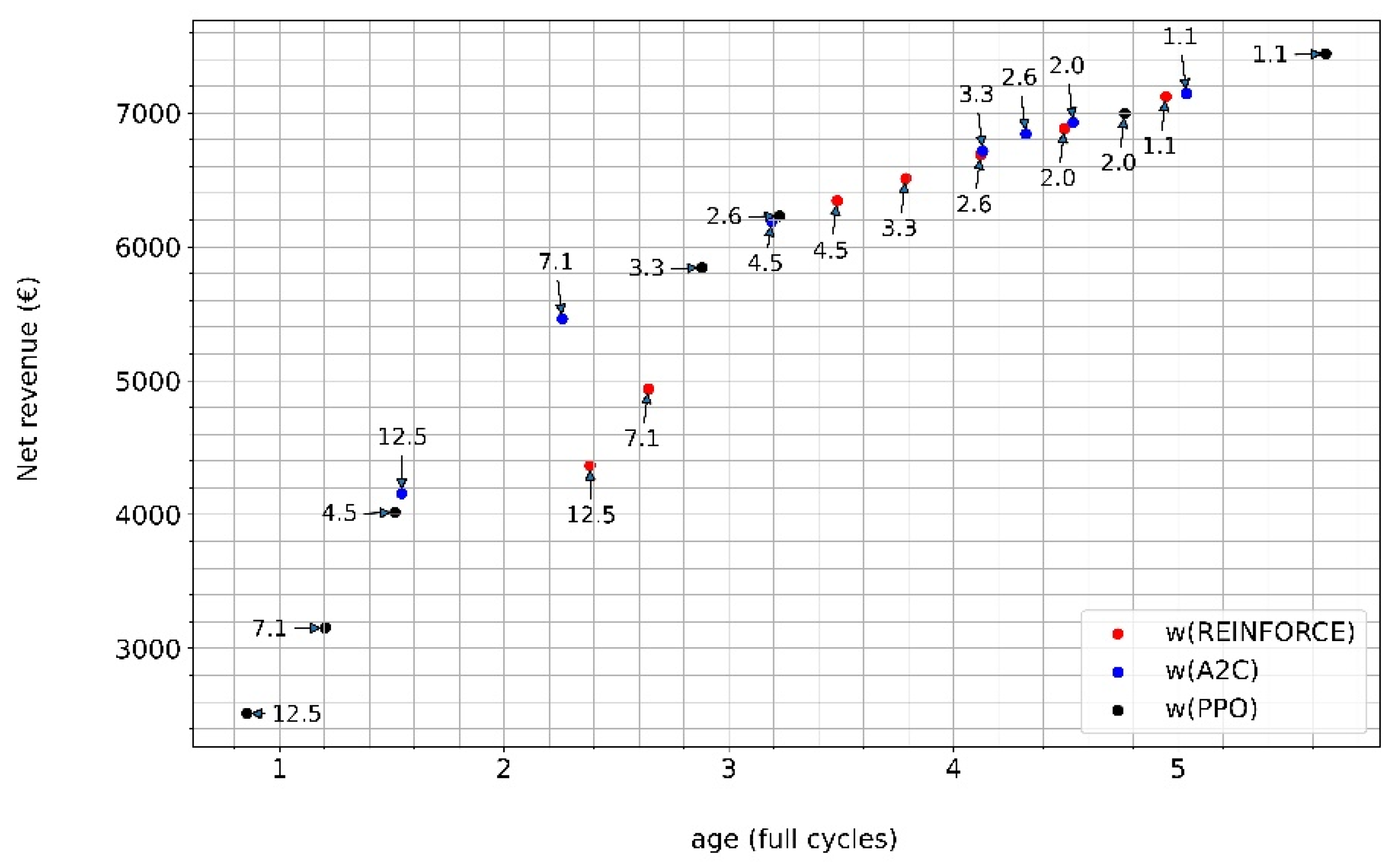
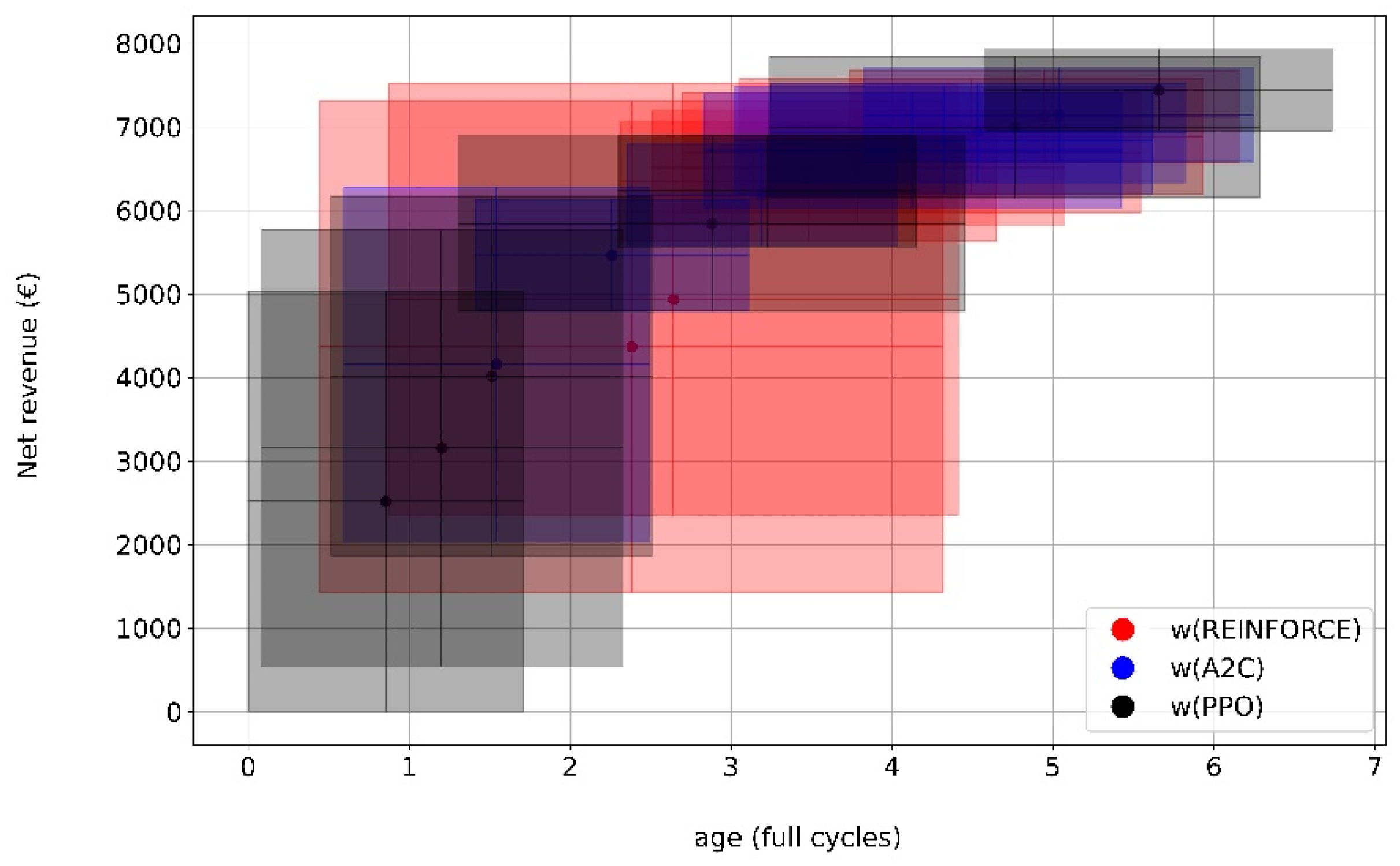
5.2. Performance Evaluation
6. Discussion
7. Conclusions
Author Contributions
Funding
Institutional Review Board Statement
Informed Consent Statement
Data Availability Statement
Conflicts of Interest
References
- Han, W.; Wik, T.; Kersten, A.; Dong, G.; Zou, C. Next-Generation Battery Management Systems: Dynamic Reconfiguration. IEEE Ind. Electron. Mag. 2020, 14, 20–31. [Google Scholar] [CrossRef]
- Ben-Idris, M.; Brown, M.; Egan, M.; Huang, Z.; Mitra, J. Utility-Scale Shared Energy Storage: Business Models for Utility-Scale Shared Energy Storage Systems and Customer Participation. IEEE Electrif. Mag. 2021, 9, 47–54. [Google Scholar] [CrossRef]
- Zhang, Y.; Gevorgian, V.; Wang, C.; Lei, X.; Chou, E.; Yang, R.; Li, Q.; Jiang, L. Grid-Level Application of Electrical Energy Storage: Example Use Cases in the United States and China. IEEE Power Energy Mag. 2017, 15, 51–58. [Google Scholar] [CrossRef]
- Tan, X.; Wu, Y.; Tsang, D.H.K. Pareto Optimal Operation of Distributed Battery Energy Storage Systems for Energy Arbitrage under Dynamic Pricing. IEEE Trans. Parallel Distrib. Syst. 2016, 27, 2103–2115. [Google Scholar] [CrossRef]
- Attarha, A.; Amjady, N.; Dehghan, S. Affinely Adjustable Robust Bidding Strategy for a Solar Plant Paired with a Battery Storage. IEEE Trans. Smart Grid 2019, 10, 2629–2640. [Google Scholar] [CrossRef]
- Filippa, A.; Hashemi, S.; Traholt, C. Economic Evaluation of Frequency Reserve Provision Using Battery Energy Storage. In Proceedings of the 2019 IEEE 2nd International Conference on Renewable Energy and Power Engineering (REPE), Toronto, ON, Canada, 2–4 November 2019; pp. 160–165. [Google Scholar]
- Chen, H.; Baker, S.; Benner, S.; Berner, A.; Liu, J. PJM Integrates Energy Storage: Their Technologies and Wholesale Products. IEEE Power Energy Mag. 2017, 15, 59–67. [Google Scholar] [CrossRef]
- Yuan, Z.; Zecchino, A.; Cherkaoui, R.; Paolone, M. Real-Time Control of Battery Energy Storage Systems to Provide Ancillary Services Considering Voltage-Dependent Capability of DC-AC Converters. IEEE Trans. Smart Grid 2021, 12, 4164–4175. [Google Scholar] [CrossRef]
- Liu, Y.; Tang, Z.; Wu, L. On Secured Spinning Reserve Deployment of Energy-Limited Resources Against Contingencies. IEEE Trans. Power Syst. 2022, 37, 518–529. [Google Scholar] [CrossRef]
- AlSkaif, T.; Crespo-Vazquez, J.L.; Sekuloski, M.; van Leeuwen, G.; Catalao, J.P.S. Blockchain-Based Fully Peer-to-Peer Energy Trading Strategies for Residential Energy Systems. IEEE Trans. Ind. Inform. 2022, 18, 231–241. [Google Scholar] [CrossRef]
- Borowski, P.F. Zonal and Nodal Models of Energy Market in European Union. Energies 2020, 13, 4182. [Google Scholar] [CrossRef]
- Mohsenian-Rad, H. Coordinated Price-Maker Operation of Large Energy Storage Units in Nodal Energy Markets. IEEE Trans. Power Syst. 2016, 31, 786–797. [Google Scholar] [CrossRef] [Green Version]
- Vedullapalli, D.T.; Hadidi, R.; Schroeder, B. Combined HVAC and Battery Scheduling for Demand Response in a Building. IEEE Trans. Ind. Appl. 2019, 55, 7008–7014. [Google Scholar] [CrossRef]
- Xu, B.; Zhao, J.; Zheng, T.; Litvinov, E.; Kirschen, D. Factoring the Cycle Aging Cost of Batteries Participating in Electricity Markets. In Proceedings of the 2018 IEEE Power & Energy Society General Meeting (PESGM), Portland, OR, USA, 5–10 August 2018; p. 1. [Google Scholar]
- Akbari-Dibavar, A.; Mohammadi-Ivatloo, B.; Anvari-Moghaddam, A.; Nojavan, S.; Vahid-Ghavidel, M.; Shafie-khah, M.; Catalao, J.P.S. Optimal Battery Storage Arbitrage Considering Degradation Cost in Energy Markets. In Proceedings of the 2020 IEEE 29th International Symposium on Industrial Electronics (ISIE), Delft, The Netherlands, 17–19 June 2020; pp. 929–934. [Google Scholar]
- Padmanabhan, N.; Ahmed, M.; Bhattacharya, K. Battery Energy Storage Systems in Energy and Reserve Markets. IEEE Trans. Power Syst. 2020, 35, 215–226. [Google Scholar] [CrossRef]
- He, G.; Chen, Q.; Kang, C.; Pinson, P.; Xia, Q. Optimal Bidding Strategy of Battery Storage in Power Markets Considering Performance-Based Regulation and Battery Cycle Life. IEEE Trans. Smart Grid 2016, 7, 2359–2367. [Google Scholar] [CrossRef] [Green Version]
- Guo, C.; Wang, X.; Zheng, Y.; Zhang, F. Optimal Energy Management of Multi-Microgrids Connected to Distribution System Based on Deep Reinforcement Learning. Int. J. Electr. Power Energy Syst. 2021, 131, 107048. [Google Scholar] [CrossRef]
- Oh, E. Reinforcement-Learning-Based Virtual Energy Storage System Operation Strategy for Wind Power Forecast Uncertainty Management. Appl. Sci. 2020, 10, 6420. [Google Scholar] [CrossRef]
- Natella, D.; Vasca, F. Battery State of Health Estimation via Reinforcement Learning. In Proceedings of the 2021 European Control Conference (ECC), Delft, The Netherlands, 29 June–2 July 2021; pp. 1657–1662. [Google Scholar]
- Aaltonen, H.; Sierla, S.; Subramanya, R.; Vyatkin, V. A Simulation Environment for Training a Reinforcement Learning Agent Trading a Battery Storage. Energies 2021, 14, 5587. [Google Scholar] [CrossRef]
- Huang, B.; Wang, J. Deep-Reinforcement-Learning-Based Capacity Scheduling for PV-Battery Storage System. IEEE Trans. Smart Grid 2021, 12, 2272–2283. [Google Scholar] [CrossRef]
- Dong, Y.; Dong, Z.; Zhao, T.; Ding, Z. A Strategic Day-Ahead Bidding Strategy and Operation for Battery Energy Storage System by Reinforcement Learning. Electr. Power Syst. Res. 2021, 196, 107229. [Google Scholar] [CrossRef]
- Knezevic, G.; Maligec, M.; Golub, V.; Topic, D. The Optimal Utilization of the Battery Storage for a Virtual Prosumer Participating on a Day-Ahead Market. In Proceedings of the 2020 International Conference on Smart Systems and Technologies (SST), Osijek, Croatia, 14–16 October 2020; pp. 155–160. [Google Scholar]
- Liu, M.; Lee, W.-J.; Lee, L.K. Financial Opportunities by Implementing Renewable Sources and Storage Devices for Households Under ERCOT Demand Response Programs Design. IEEE Trans. Ind. Appl. 2014, 50, 2780–2787. [Google Scholar] [CrossRef]
- Motta, S.; Aro, M.; Evens, C.; Hentunen, A.; Ikäheimo, J. A Cost-Benefit Analysis Of Large-Scale Battery Energy Storage Systems for Frequency Markets. In Proceedings of the CIRED 2021—The 26th International Conference and Exhibition on Electricity Distribution; Institution of Engineering and Technology, Online Conference, 20–23 September 2021; pp. 3130–3134. [Google Scholar]
- Meng, Z.; Xu, Q.; Mao, T.; Li, M.; He, D. Research on the Full-Life-Cycle Operation Benefit Estimation of the Battery Energy Storage Station Anticipating the Ancillary Service Market in China. In Proceedings of the 2019 IEEE 3rd International Electrical and Energy Conference (CIEEC), Beijing, China, 7–9 September 2019; pp. 1086–1090. [Google Scholar]
- Moolman, J.; Das, K.; Sørensen, P. Operation of Battery Storage in Hybrid Power Plant in Australian Electricity Market. In Proceedings of the 9th Renewable Power Generation Conference (RPG Dublin Online 2021), Institution of Engineering and Technology, Online Conference, 1–2 March 2021; pp. 349–354. [Google Scholar]
- Goujard, G.; Badoual, M.D.; Janin, K.A.; Schwarz, S.; Moura, S.J. Optimal Siting, Sizing and Bid Scheduling of a Price-Maker Battery on a Nodal Wholesale Market. In Proceedings of the 2021 American Control Conference (ACC), Online Conference, 25–28 May 2021; pp. 602–607. [Google Scholar]
- Lujano-Rojas, J.M.; Yusta, J.M.; Dominguez-Navarro, J.A.; Osorio, G.J.; Shafie-khah, M.; Wang, F.; Catalao, J.P.S. Combining Genetic and Gravitational Search Algorithms for the Optimal Management of Battery Energy Storage Systems in Real-Time Pricing Markets. In Proceedings of the 2020 IEEE Industry Applications Society Annual Meeting, Detroit, MI, USA, 10–16 October 2020; pp. 1–7. [Google Scholar]
- Benini, M.; Canevese, S.; Cirio, D.; Gatti, A. Participation of Battery Energy Storage Systems in the Italian Balancing Market: Management Strategies and Economic Results. In Proceedings of the 2018 IEEE International Conference on Environment and Electrical Engineering and 2018 IEEE Industrial and Commercial Power Systems Europe (EEEIC/I&CPS Europe), Palermo, Italy, 12–15 June 2018; pp. 1–6. [Google Scholar]
- Mohsenian-Rad, H. Optimal Bidding, Scheduling, and Deployment of Battery Systems in California Day-Ahead Energy Market. IEEE Trans. Power Syst. 2016, 31, 442–453. [Google Scholar] [CrossRef] [Green Version]
- Robson, S.; Alharbi, A.M.; Gao, W.; Khodaei, A.; Alsaidan, I. Economic Viability Assessment of Repurposed EV Batteries Participating in Frequency Regulation and Energy Markets. In Proceedings of the 2021 IEEE Green Technologies Conference (GreenTech), Denver, CO, USA, 7–9 April 2021; pp. 424–429. [Google Scholar]
- Khalilisenobari, R.; Wu, M. Impact of Battery Degradation on Market Participation of Utility-Scale Batteries: Case Studies. In Proceedings of the 2020 52nd North American Power Symposium (NAPS), Tempe, AZ, USA, 11–14 April 2021; pp. 1–6. [Google Scholar]
- Gupta, A.; Vaishya, S.R.; Gupta, M.; Abhyankar, A.R. Participation of Battery Energy Storage Technologies in Co-Optimized Energy and Reserve Markets. In Proceedings of the 2020 21st National Power Systems Conference (NPSC), Gandhinagar, India, 17–19 December 2020; pp. 1–6. [Google Scholar]
- Padmanabhan, N.; Bhattacharya, K. Including Demand Response and Battery Energy Storage Systems in Uniform Marginal Price Based Electricity Markets. In Proceedings of the 2021 IEEE Power & Energy Society Innovative Smart Grid Technologies Conference (ISGT), Washington, DC, USA, 16–18 February 2021; pp. 1–5. [Google Scholar]
- Kadri, A.; Mohammadi, F. Battery Storage System Optimization for Multiple Revenue Streams and Savings. In Proceedings of the 2020 IEEE Canadian Conference on Electrical and Computer Engineering (CCECE), London, ON, Canada, 30 August–2 September 2020; pp. 1–5. [Google Scholar]
- Prudhviraj, D.; Kiran, P.B.S.; Pindoriya, N.M. Stochastic Energy Management of Microgrid with Nodal Pricing. J. Mod. Power Syst. Clean Energy 2020, 8, 102–110. [Google Scholar] [CrossRef]
- Chen, C.; Wei, Z.; Knoll, A.C. Charging Optimization for Li-Ion Battery in Electric Vehicles: A Review. IEEE Trans. Transp. Electrif. 2021, 1. [Google Scholar] [CrossRef]
- Wu, J.; Wei, Z.; Li, W.; Wang, Y.; Li, Y.; Sauer, D.U. Battery Thermal- and Health-Constrained Energy Management for Hybrid Electric Bus Based on Soft Actor-Critic DRL Algorithm. IEEE Trans. Ind. Inform. 2021, 17, 3751–3761. [Google Scholar] [CrossRef]
- Nefedov, E.; Sierla, S.; Vyatkin, V. Internet of Energy Approach for Sustainable Use of Electric Vehicles as Energy Storage of Prosumer Buildings. Energies 2018, 11, 2165. [Google Scholar] [CrossRef] [Green Version]
- Ansari, M.; Al-Awami, A.T.; Sortomme, E.; Abido, M.A. Coordinated Bidding of Ancillary Services for Vehicle-to-Grid Using Fuzzy Optimization. IEEE Trans. Smart Grid 2015, 6, 261–270. [Google Scholar] [CrossRef]
- Zeng, M.; Leng, S.; Maharjan, S.; Gjessing, S.; He, J. An Incentivized Auction-Based Group-Selling Approach for Demand Response Management in V2G Systems. IEEE Trans. Ind. Inform. 2015, 11, 1554–1563. [Google Scholar] [CrossRef] [Green Version]
- Rassaei, F.; Soh, W.-S.; Chua, K.-C. Demand Response for Residential Electric Vehicles With Random Usage Patterns in Smart Grids. IEEE Trans. Sustain. Energy 2015, 6, 1367–1376. [Google Scholar] [CrossRef]
- Zhou, M.; Wu, Z.; Wang, J.; Li, G. Forming Dispatchable Region of Electric Vehicle Aggregation in Microgrid Bidding. IEEE Trans. Ind. Inform. 2021, 17, 4755–4765. [Google Scholar] [CrossRef]
- Tan, J.; Wang, L. A Game-Theoretic Framework for Vehicle-to-Grid Frequency Regulation Considering Smart Charging Mechanism. IEEE Trans. Smart Grid 2017, 8, 2358–2369. [Google Scholar] [CrossRef]
- Donadee, J.; Ilic, M.D. Stochastic Optimization of Grid to Vehicle Frequency Regulation Capacity Bids. IEEE Trans. Smart Grid 2014, 5, 1061–1069. [Google Scholar] [CrossRef]
- Sortomme, E.; El-Sharkawi, M.A. Optimal Charging Strategies for Unidirectional Vehicle-to-Grid. IEEE Trans. Smart Grid 2011, 2, 131–138. [Google Scholar] [CrossRef]
- De Silva, D.; Sierla, S.; Alahakoon, D.; Osipov, E.; Yu, X.; Vyatkin, V. Toward Intelligent Industrial Informatics: A Review of Current Developments and Future Directions of Artificial Intelligence in Industrial Applications. IEEE Ind. Electron. Mag. 2020, 14, 57–72. [Google Scholar] [CrossRef]
- Kahawala, S.; de Silva, D.; Sierla, S.; Alahakoon, D.; Nawaratne, R.; Osipov, E.; Jennings, A.; Vyatkin, V. Robust Multi-Step Predictor for Electricity Markets with Real-Time Pricing. Energies 2021, 14, 4378. [Google Scholar] [CrossRef]
- Kempitiya, T.; Sierla, S.; de Silva, D.; Yli-Ojanperä, M.; Alahakoon, D.; Vyatkin, V. An Artificial Intelligence Framework for Bidding Optimization with Uncertainty in Multiple Frequency Reserve Markets. Appl. Energy 2020, 280, 115918. [Google Scholar] [CrossRef]
- Beltrán, S.; Castro, A.; Irizar, I.; Naveran, G.; Yeregui, I. Framework for Collaborative Intelligence in Forecasting Day-Ahead Electricity Price. Appl. Energy 2022, 306, 118049. [Google Scholar] [CrossRef]
- Haputhanthri, D.; de Silva, D.; Sierla, S.; Alahakoon, D.; Nawaratne, R.; Jennings, A.; Vyatkin, V. Solar Irradiance Nowcasting for Virtual Power Plants Using Multimodal Long Short-Term Memory Networks. Front. Energy Res. 2021, 9, 722212. [Google Scholar] [CrossRef]
- Wood, D.A. Trend Decomposition Aids Short-Term Countrywide Wind Capacity Factor Forecasting with Machine and Deep Learning Methods. Energy Convers. Manag. 2022, 253, 115189. [Google Scholar] [CrossRef]
- Pallonetto, F.; Jin, C.; Mangina, E. Forecast Electricity Demand in Commercial Building with Machine Learning Models to Enable Demand Response Programs. Energy AI 2022, 7, 100121. [Google Scholar] [CrossRef]
- Cao, J.; Harrold, D.; Fan, Z.; Morstyn, T.; Healey, D.; Li, K. Deep Reinforcement Learning-Based Energy Storage Arbitrage With Accurate Lithium-Ion Battery Degradation Model. IEEE Trans. Smart Grid 2020, 11, 4513–4521. [Google Scholar] [CrossRef]
- Wang, Y.; Lin, X.; Pedram, M. A Near-Optimal Model-Based Control Algorithm for Households Equipped With Residential Photovoltaic Power Generation and Energy Storage Systems. IEEE Trans. Sustain. Energy 2016, 7, 77–86. [Google Scholar] [CrossRef]
- Chasparis, G.C.; Lettner, C. Reinforcement-Learning-Based Optimization for Day-Ahead Flexibility Extraction in Battery Pools. IFAC-PapersOnLine 2020, 53, 13351–13358. [Google Scholar] [CrossRef]
- Lee, S.; Choi, D.-H. Energy Management of Smart Home with Home Appliances, Energy Storage System and Electric Vehicle: A Hierarchical Deep Reinforcement Learning Approach. Sensors 2020, 20, 2157. [Google Scholar] [CrossRef] [PubMed] [Green Version]
- Lee, S.; Choi, D.-H. Reinforcement Learning-Based Energy Management of Smart Home with Rooftop Solar Photovoltaic System, Energy Storage System, and Home Appliances. Sensors 2019, 19, 3937. [Google Scholar] [CrossRef] [Green Version]
- Yang, J.J.; Yang, M.; Wang, M.X.; Du, P.J.; Yu, Y.X. A Deep Reinforcement Learning Method for Managing Wind Farm Uncertainties through Energy Storage System Control and External Reserve Purchasing. Int. J. Electr. Power Energy Syst. 2020, 119, 105928. [Google Scholar] [CrossRef]
- Liu, W.; Zhuang, P.; Liang, H.; Peng, J.; Huang, Z. Distributed Economic Dispatch in Microgrids Based on Cooperative Reinforcement Learning. IEEE Trans. Neural Netw. Learn. Syst. 2018, 29, 2192–2203. [Google Scholar] [CrossRef]
- Zhou, S.; Hu, Z.; Gu, W.; Jiang, M.; Zhang, X.-P. Artificial Intelligence Based Smart Energy Community Management: A Reinforcement Learning Approach. CSEE J. Power Energy Syst. 2019, 5, 1–10. [Google Scholar] [CrossRef]
- Wang, S.; Du, L.; Fan, X.; Huang, Q. Deep Reinforcement Scheduling of Energy Storage Systems for Real-Time Voltage Regulation in Unbalanced LV Networks With High PV Penetration. IEEE Trans. Sustain. Energy 2021, 12, 2342–2352. [Google Scholar] [CrossRef]
- Qiu, X.; Nguyen, T.A.; Crow, M.L. Heterogeneous Energy Storage Optimization for Microgrids. IEEE Trans. Smart Grid 2016, 7, 1453–1461. [Google Scholar] [CrossRef]
- Hofstetter, J.; Bauer, H.; Li, W.; Wachtmeister, G. Energy and Emission Management of Hybrid Electric Vehicles Using Reinforcement Learning. IFAC-PapersOnLine 2019, 52, 19–24. [Google Scholar] [CrossRef]
- Zhou, J.; Xue, S.; Xue, Y.; Liao, Y.; Liu, J.; Zhao, W. A Novel Energy Management Strategy of Hybrid Electric Vehicle via an Improved TD3 Deep Reinforcement Learning. Energy 2021, 224, 120118. [Google Scholar] [CrossRef]
- Hua, H.; Qin, Y.; Hao, C.; Cao, J. Optimal Energy Management Strategies for Energy Internet via Deep Reinforcement Learning Approach. Appl. Energy 2019, 239, 598–609. [Google Scholar] [CrossRef]
- Muriithi, G.; Chowdhury, S. Optimal Energy Management of a Grid-Tied Solar PV-Battery Microgrid: A Reinforcement Learning Approach. Energies 2021, 14, 2700. [Google Scholar] [CrossRef]
- Yang, T.; Zhao, L.; Li, W.; Zomaya, A.Y. Dynamic Energy Dispatch Strategy for Integrated Energy System Based on Improved Deep Reinforcement Learning. Energy 2021, 235, 121377. [Google Scholar] [CrossRef]
- Chen, Z.; Hu, H.; Wu, Y.; Xiao, R.; Shen, J.; Liu, Y. Energy Management for a Power-Split Plug-In Hybrid Electric Vehicle Based on Reinforcement Learning. Appl. Sci. 2018, 8, 2494. [Google Scholar] [CrossRef] [Green Version]
- Wu, J.; Wei, Z.; Liu, K.; Quan, Z.; Li, Y. Battery-Involved Energy Management for Hybrid Electric Bus Based on Expert-Assistance Deep Deterministic Policy Gradient Algorithm. IEEE Trans. Veh. Technol. 2020, 69, 12786–12796. [Google Scholar] [CrossRef]
- Wei, Z.; Quan, Z.; Wu, J.; Li, Y.; Pou, J.; Zhong, H. Deep Deterministic Policy Gradient-DRL Enabled Multiphysics-Constrained Fast Charging of Lithium-Ion Battery. IEEE Trans. Ind. Electron. 2022, 69, 2588–2598. [Google Scholar] [CrossRef]
- Karhula, N.; Sierla, S.; Vyatkin, V. Validating the Real-Time Performance of Distributed Energy Resources Participating on Primary Frequency Reserves. Energies 2021, 14, 6914. [Google Scholar] [CrossRef]
- Giovanelli, C.; Kilkki, O.; Sierla, S.; Seilonen, I.; Vyatkin, V. Task Allocation Algorithm for Energy Resources Providing Frequency Containment Reserves. IEEE Trans. Ind. Inform. 2018, 15, 677–688. [Google Scholar] [CrossRef]
- Giovanelli, C.; Sierla, S.; Ichise, R.; Vyatkin, V. Exploiting Artificial Neural Networks for the Prediction of Ancillary Energy Market Prices. Energies 2018, 11, 1906. [Google Scholar] [CrossRef] [Green Version]
- Hua, H.; Qin, Z.; Dong, N.; Qin, Y.; Ye, M.; Wang, Z.; Chen, X.; Cao, J. Data-Driven Dynamical Control for Bottom-up Energy Internet System. IEEE Trans. Sustain. Energy 2022, 13, 315–327. [Google Scholar] [CrossRef]
- Chen, W.; Wu, N.; Huang, Y. Real-Time Optimal Dispatch of Microgrid Based on Deep Deterministic Policy Gradient Algorithm. In Proceedings of the 2021 International Conference on Big Data and Intelligent Decision Making (BDIDM), Guilin, China, 23–25 July 2021; pp. 24–28. [Google Scholar]
- Yi, Y.; Verbic, G.; Chapman, A.C. Optimal Energy Management Strategy for Smart Home with Electric Vehicle. In Proceedings of the 2021 IEEE Madrid PowerTech, Madrid, Spain, 28 June–2 July 2021; pp. 1–6. [Google Scholar]
- Opalic, S.M.; Goodwin, M.; Jiao, L.; Nielsen, H.K.; Lal Kolhe, M. A Deep Reinforcement Learning Scheme for Battery Energy Management. In Proceedings of the 2020 5th International Conference on Smart and Sustainable Technologies (SpliTech), Split, Croatia, 23–26 September 2020; pp. 1–6. [Google Scholar]
- Sutton, R.; Barto, A. Reinforcement Learning: An Introduction; MIT Press: Cambridge, MA, USA, 2020. [Google Scholar]
- Omar, N.; Monem, M.A.; Firouz, Y.; Salminen, J.; Smekens, J.; Hegazy, O.; Gaulous, H.; Mulder, G.; van den Bossche, P.; Coosemans, T.; et al. Lithium Iron Phosphate Based Battery—Assessment of the Aging Parameters and Development of Cycle Life Model. Appl. Energy 2014, 113, 1575–1585. [Google Scholar] [CrossRef]
- Tremblay, O.; Dessaint, L.-A. Experimental Validation of a Battery Dynamic Model for EV Applications. World Electr. Veh. J. 2009, 3, 289–298. [Google Scholar] [CrossRef] [Green Version]
- MathWorks Battery. Available online: https://www.mathworks.com/help/physmod/sps/powersys/ref/battery.html (accessed on 16 May 2022).

| Symbol | Description |
|---|---|
| SoC | State of charge of the battery in percent |
| DoD | Depth of discharge—the complement of SoC, i.e., DoD = 100% − SoC |
| i | Charging/discharging current of the battery—negative values mean discharging |
| u | Voltage of the battery |
| P | Charging/discharging power of the battery, P = u i. |
| R | Hours since the battery last rested, i.e., did not participate on the market and was charged/discharged to 50% SoC with constant power |
| FCRact | Actual price (EUR/MW)on that particular hour on the Finnish FCR-N market |
| FCRfcast | Forecasted price (EUR/MW) on that particular hour on the Finnish FCR-N market |
| T | Number of seconds in one market interval of FCR-N. At the time of writing, T = 3600 |
| C | Capacity of the bid made to the FCR-N market. The capacity is in MW and specifies the value of P when the full activation is required. The full activation occurs when the power grid frequency deviation exceeds the limit at which the FCR-N technical specification requires 100% activation of the capacity. In our RL formulation, four discrete values for capacity are used: 0 MW, 0.3 MW, 0.4 MW and 0.5 MW |
| age | Age of the battery (equivalent full cycles) |
| pen | Market penalty for failing to deliver the capacity C. The penalty is expressed as a percentage of the duration of the market interval, during which the battery is not available due to the SoC exceeding a minimum or maximum threshold |
| A | Aging penalty (component of the reward function) |
| w | Weight for the aging penalty A |
| Symbol | Description | Constant Value |
|---|---|---|
| H | The cycle number constant in cycles | YES |
| The exponent factor for DoD | YES | |
| The Arrhenius rate constant for the cycle number | YES | |
| Reference temperature | YES | |
| Ambient temperature | YES | |
| The average discharge current in A during a half cycle duration | NO | |
| The average charge current in A during a half cycle duration | NO | |
| The exponent factor for the discharge current | YES | |
| The exponent factor for the charge current | YES |
| REINFORCE | A2C | PPO | |
|---|---|---|---|
| Gamma (discount factor) | 0.5 | 0.5 | 0.5 |
| Alpha (learning rate) | 0.01 | 0.01 | 0.01 |
| Input states | 2 | 2 | 2 |
| Number of hidden layers | 1 | 1 | 1 |
| Nodes on hidden layer 1 | 20 | 20 | 20 |
| Hidden layer activation function | Sigmoid | Sigmoid | Sigmoid |
| Output actions | 4 | 4 | 4 |
| Output layer activation function | Softmax | Softmax | Softmax |
| Dropout | Not used | Not used | Not used |
| Optimizer | Adam | Adam | Adam |
| Number of seeds | 10 | 10 | 10 |
| N (length of memory) | 24 | ||
| Batch size | 6 | ||
| Number of epochs | 4 | ||
| Gae lambda | 0.95 | ||
| Policy clip | 0.2 |
| Nominal voltage (V) | 772.8 |
| Rated capacity (Ah) | 700.0 |
| Battery response time (s) | 2.0 |
| Sample time (s) | 1.0 |
| Maximum capacity | 700.0 |
| Cut-off voltage (V) | 504.0 |
| Fully charged voltage | 907.4 |
| Nominal discharge current (A) | 304.3478 |
| Internal resistance (Ohms) | 0.01104 |
| Capacity (Ah) at nominal voltage | 633.0435 |
| Exponential zone [voltage (V), capacity (Ah)] | [834.9222, 34.3913] |
| Initial battery age (equivalent full cycles) | 0.0 |
| Aging model sampling time (s) | 2.0 |
| Ambient temperatur Ta1 (deg. C) | 25.0 |
| Capacity at End of Life (EOL) (Ah) | 633.0435 × 0.9 |
| Internal resistance at EOL (Ohms) | 0.01104 × 1.2 |
| Charge current (nominal, maximum) [Ic (A), Icmax (A)] | [304.3478, 304.3478 × 3] |
| Discharge current (nominal, maximum) [Id (A), Idmax (A)] | [304.3478, 304.3478 × 3] |
| Cycle life at 100% DOD, Ic and Id (cycles) | 20,000.0 |
| Cycle life at 25% DOD, Ic and Id (cycles) | 40,000.0 |
| Cycle life at 100% DOD, Ic and Idmax (cycles) | 8000.0 |
| Cycle life at 100% DOD, Icmax and Id (cycles) | 8000.0 |
| Ambient temperatur Ta2 (deg. C) | 45.0 |
| Cycle life at 100% DOD, Ic and Id (cycles) | 950.0 |
| Algorithm | REINFORCE | A2C | PPO |
|---|---|---|---|
| Training reward | 40.03 | 40.78 | 40.72 |
| Training rewards std | 15.17 | 17.74 | 14.05 |
| Validation reward | 1878.87 | 1917.16 | 1907.51 |
| Validation reward std | 68.03 | 101.43 | 187.03 |
Publisher’s Note: MDPI stays neutral with regard to jurisdictional claims in published maps and institutional affiliations. |
© 2022 by the authors. Licensee MDPI, Basel, Switzerland. This article is an open access article distributed under the terms and conditions of the Creative Commons Attribution (CC BY) license (https://creativecommons.org/licenses/by/4.0/).
Share and Cite
Aaltonen, H.; Sierla, S.; Kyrki, V.; Pourakbari-Kasmaei, M.; Vyatkin, V. Bidding a Battery on Electricity Markets and Minimizing Battery Aging Costs: A Reinforcement Learning Approach. Energies 2022, 15, 4960. https://doi.org/10.3390/en15144960
Aaltonen H, Sierla S, Kyrki V, Pourakbari-Kasmaei M, Vyatkin V. Bidding a Battery on Electricity Markets and Minimizing Battery Aging Costs: A Reinforcement Learning Approach. Energies. 2022; 15(14):4960. https://doi.org/10.3390/en15144960
Chicago/Turabian StyleAaltonen, Harri, Seppo Sierla, Ville Kyrki, Mahdi Pourakbari-Kasmaei, and Valeriy Vyatkin. 2022. "Bidding a Battery on Electricity Markets and Minimizing Battery Aging Costs: A Reinforcement Learning Approach" Energies 15, no. 14: 4960. https://doi.org/10.3390/en15144960
APA StyleAaltonen, H., Sierla, S., Kyrki, V., Pourakbari-Kasmaei, M., & Vyatkin, V. (2022). Bidding a Battery on Electricity Markets and Minimizing Battery Aging Costs: A Reinforcement Learning Approach. Energies, 15(14), 4960. https://doi.org/10.3390/en15144960