Abstract
When a single-phase grounding fault occurs in a resonant grounding system, the determination of the fault location remains a significant challenge due to the small fault current and the instability of the grounding arc. In order to solve the problem of low protection sensitivity when a high-resistance grounding fault occurs in a resonant grounding system, this paper proposes a fault location method based on the combination of dynamic time warping (DTW) distance and fuzzy C-means (FCM) clustering. By analyzing the characteristics of the zero-sequence current upstream and downstream of the fault point when a single-phase grounding fault occurs in the resonant grounding system, it is concluded that the waveform similarity on both sides of the fault point is low. DTW distance can be used to measure the similarity of two time series, and has the characteristics of good fault tolerance and synchronization error tolerance. According to the rule that the DTW value of faulty section is much larger than that of nonfaulty sections, FCM clustering is used to classify the DTW value of each section. The membership degree matrix and cluster centers are obtained. In the membership degree matrix, the section corresponding to the data in a class of their own is the faulty section, and all other data correspond to the nonfaulty section; otherwise, it is a fault occurring at the end of the line. The simulation results of MATLAB/Simulink and the field data test show that the method can accurately locate the faulty section.
1. Introduction
The neutral point grounding modes of China’s distribution network mainly include direct grounding, nongrounding, small-resistance grounding and resonance grounding [1]. When a single-phase ground fault occurs in the resonant system, the system can run with the fault for a period of time, and the power supply reliability is high [2]. However, due to the arc-extinguishing effect of the arc suppression coil, the fault current is small, especially when a high-resistance grounding fault occurs, and the transient information is not obvious, which increases the difficulty of faulty line selection and faulty section location [3].
At present, the protection and processing of single-phase grounding faults in small-current grounding systems can be divided into two categories: active and passive positioning [4]. Among them, the active positioning method is based on the signal characteristics of the active injection system. This includes the addition function method [5], S injection method [6], etc. Such methods are greatly affected by the distribution network structure and detection equipment, and the positioning effect is not ideal. The passive positioning method seeks to locate the faulty section according to the collected voltage and current signals. It mainly includes the correlation coefficient method [7], transient power direction method [8], frequency method [9] and so on. Among them, the correlation coefficient method introduces the correlation coefficient to measure the degree of correlation between the feature quantities of the monitoring points, and it locates the faulty section accordingly. The transient power direction method locates the faulty section according to the different characteristics of the upstream and downstream transient power directions of the fault point. The frequency method uses the current frequency difference upstream and downstream of the fault point to locate the faulty section. The above fault location method is greatly affected by the fault conditions, reflecting the weak transition resistance capability, and brings challenges to the determination of the fault location as the distributed power source is connected to the distribution network [10].
In order to improve the sensitivity of single-phase high-resistance grounding fault locations, this paper proposes a faulty section location method for resonant grounding systems based on dynamic time warping distance. Firstly, the zero-sequence current of each monitoring point of the faulty line is projected onto the transient zero-sequence voltage of the busbar by the transient projection method. Then, we calculate the DTW distance between the projection values of each monitoring point, and then perform FCM clustering on it to obtain the cluster center and membership degree matrix. The faulty section can be located by using the membership degree matrix. The MATLAB/Simulink simulation test and the field data test verify the feasibility of the method. The main contributions of this paper are summarized as follows:
- We are able to determine the faulty section or line end fault under diverse fault conditions;
- The method is applicable for single-phase grounding faults in a distribution network with distributed generation connected;
- The faulty section location method proposed in this paper is suitable for high-resistance grounding faults, reflecting the transition resistance capability of up to 5000 Ω;
- Under extreme fault conditions, the faulty section location accuracy of the method proposed in this paper is higher than that of the existing traditional methods.
2. Materials and Methods
2.1. Characteristics of Single-Phase Grounding Fault Current in Resonant Grounding System
In order to locate the faulty section, the fault current must be analyzed when a single-phase-to-ground fault occurs in a resonant grounded system. The single-phase grounding fault transient equivalent circuit of the resonant grounding system is shown in Figure 1. Suppose that line 3 has a single-phase ground fault at point F, and M, N, P and E are monitoring points.
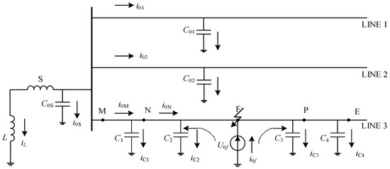
Figure 1.
Transient equivalent circuit of single-phase grounding fault in resonant grounding system.
Here,
C0s is the ground capacitance of the generator;
C01, C02 are the ground capacitances of lines 1 and 2, respectively;
C1, C2, C3 and C4 are the ground capacitances of MN, NF, FP and PE sections in line 3, respectively;
L is the inductance of the arc suppression coil.
According to the equivalent circuit, the zero-sequence current relationship between M and N is as follows:
In Equation (1), i0M is the sum of the zero-sequence-to-ground capacitance currents of all nonfaulty lines, and iC1 is the zero-sequence capacitive current of section MN to ground. Due to the small distance between sampling points, iC1 is very small compared to i0M and can be ignored, so i0M ≈ i0N, i.e., the zero-sequence current similarity of the two adjacent monitoring points, M and N, is very high.
However, due to the single-phase ground fault at point F, a virtual voltage source is generated. The dotted line in Figure 1 represents the zero-sequence current flowing from the fault point; part of it flows from the fault point to the busbar direction, while the other part flows from the fault point to the end of the line. Therefore, the transient zero-sequence currents detected at points N and P have opposite polarities, and the similarity is very low. From the above analysis, it can be seen that the similarity of the zero-sequence currents at both ends of the faulty section is low, and the similarity of the zero-sequence currents at both ends of the nonfaulty section is high. The above current distribution law will not be changed when the arc suppression coil is connected to the power system [11].
2.2. The Principle of Fault Location
2.2.1. Transient Signal Preprocessing
As the transition resistance increases, the magnitude of the zero-sequence current will become smaller. The difference between the transient information of the faulty section and the nonfaulty section will become smaller, which makes it difficult to locate the fault. In order to overcome the problems of inconspicuous transient signals and low protection sensitivity caused by high-resistance ground faults, this paper selects the transient zero-sequence voltage of the busbar, which is less affected by the transition resistance than the zero-sequence current transient signal. Projecting the transient zero-sequence current of each monitoring point of the faulty line onto the busbar transient zero-sequence voltage can more clearly characterize the fault characteristics. Therefore, it can compensate for the shortcoming whereby the transient zero-sequence current is too small when the high-resistance ground fault occurs.
The schematic diagram of the transient projection method is shown in Figure 2. α is the angle between the vectors and . is the projection size of onto , and the projection vector is .
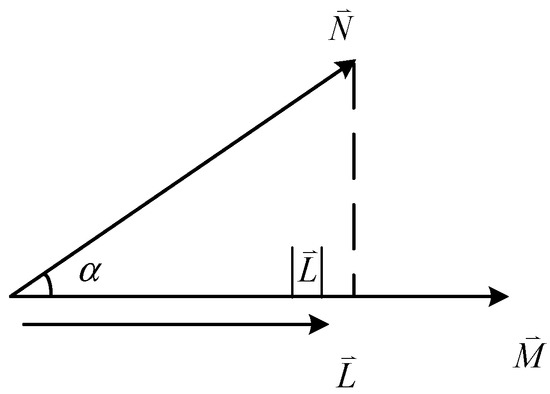
Figure 2.
Projection vector diagram.
The relationship between the variables can be obtained from Figure 2.
Then, the calculation formula of the projection of onto is
where is the inner product of vectors and . The projection of the line transient zero-sequence current onto the busbar transient zero-sequence voltage can be calculated by Equation (3) [12]. is analogous to the zero-sequence current of the monitoring point (i = 1, 2, …, n), and is analogous to the zero-sequence voltage of busbar . Then, the projection value of the transient zero-sequence current of each monitoring point on the transient zero-sequence voltage of the busbar is
The transient projection method has a better effect on transient signals and is also suitable for high-resistance ground faults.
2.2.2. Dynamic Time Warping Distance
Principle of DTW Algorithm
Dynamic time warping distance was first proposed by Japanese scholars in the 1960s and applied to the field of speech recognition. Suppose that there are two time series and with sequence lengths m and n, respectively. DTW uses the idea of dynamic programming to adjust the correspondence between the two sequences to obtain an optimal path that minimizes the distance between the two sequences along the path [13]. A schematic diagram of the DTW path is shown in Figure 3.
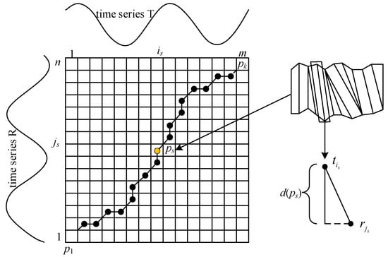
Figure 3.
Schematic diagram of DTW path.
In the path diagram shown in Figure 3, the path formed by the black dots is the curved path, i.e., , where Ps is the s-th point in the curved path, and its co-ordinate is ps = (is,js); it indicates that the is-th point in the sequence T corresponds to the js-th point in the sequence R. Then, the distance between two points is ; thereby, the distance matrix D of the corresponding points of the two sequences can be obtained.
The selection of the curved path should satisfy the following constraints:
- (1)
- Boundary conditions: the starting point is (1, 1) and the end point is (m, n).
- (2)
- Boundedness: the sequence of time series cannot be changed. , where K is the total number of steps of the curved path P.
- (3)
- Monotonicity: If the curved path moves from point ps to the next point ps+1, it must satisfy is+1 ≥ is, js+1 ≥ js, i.e., phenomenon ① in Figure 4 is not allowed.
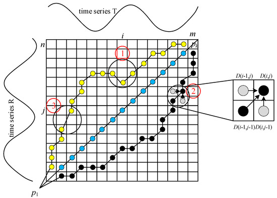 Figure 4. Schematic diagram of DTW constraint path.
 - (4)
- Continuity: The path can only proceed along adjacent points, i.e., in Figure 3, if the ps in the curved path reaches the next step ps+1, it needs to satisfy is+1 − is ≤ 1, js+1 − js ≤ 1. As shown in Figure 4, in order to ensure continuity, in ②, the path to point D(i, j) must pass through one of D(i − 1, j − 1), D(i − 1, j), D(i, j − 1), and the discontinuity in ③ is not allowed.
There will be multiple paths P between the two time series that satisfy the constraints, and all paths can form a path space W, where the shortest path length is the DTW distance between the two time series:
The larger the DTW value, the lower the similarity between the two time series, and the smaller the DTW value, the higher the similarity between the time series. Because DTW distance has high sensitivity and strong resistance to synchronization error, it can be used to identify the similarity of waveforms.
Relationship between DTW Distance and Zero-Sequence Current Difference
When a single-phase grounding fault occurs in the resonant grounding system, the frequency and amplitude of the zero-sequence current on both sides of the fault point are significantly different, so that the faulty section can be located. The zero-sequence currents flowing through the two monitoring points are represented by the new sequences and , respectively. The amplitude H increases from 1 to 10, and k takes 1, 5, 10 and 100, respectively [14]. The relationship between the exploration and the zero-sequence current amplitude and frequency difference is shown in Figure 5.
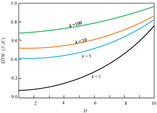
Figure 5.
Relationship between DTW distance and the amplitude and frequency difference of zero-sequence current.
By analyzing Figure 5, it can be seen that when k is constant, as H increases, the amplitude difference in the two sequences increases, and the DTW distance increases accordingly; when H is constant, as k increases, the representative frequency difference increases, and the DTW distance also increases. The frequency and amplitude of the zero-sequence current on both sides of the fault point are significantly different, so the DTW distance is large. However, the difference in the frequency and amplitude of the zero-sequence current on the same side of the fault point is small, and the DTW distance is small. This can be used as a criterion to locate the faulty section.
2.2.3. FCM Clustering
Fuzzy C-means clustering is referred to as FCM clustering; it is widely used in the cluster analysis of data [15]. FCM clustering classifies the input data into different cluster centers and iteratively corrects the membership degree matrix and the cluster centers to reduce the weighted distance of membership between the data and the cluster centers, so as to classify the data.
In this paper, FCM clustering is used to divide the DTW value of each section of the faulty line into two categories. The objective function of FCM clustering is
Among the terms, X is the membership degree matrix; Y is the cluster center; Q is the weighting coefficient, which is generally taken as 2. yj is the j-th cluster center, and the cluster center and membership degree matrix are obtained after iteration.
Using the Lagrange multiplier method, the cluster center Y is obtained as
The membership degree matrix X is
The two cluster centers in Y are the cluster center of the faulty section and the cluster center of the nonfaulty section, respectively. xji is the membership degree of the i-th section to the j-th cluster center. When a single-phase grounding fault occurs in the resonant grounding system, the DTW value of the faulty section is large, and the DTW value of the nonfaulty section is small. Therefore, the section corresponding to the value of its own kind in the membership degree matrix is the faulty section, and all the other data correspond to the nonfaulty section—this enables fault localization. The advantage of the membership degree matrix is that the fault location determination can be completed without setting thresholds.
2.2.4. Faulty Section Location Process
Based on the above analysis, it can be seen that when a single-phase grounding fault occurs in the resonant grounding system, the fault location determination can be carried out by using the data of their own kind in the membership degree matrix. A flowchart of the fault location method is shown in Figure 6. The specific location process is as follows:
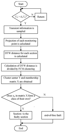
Figure 6.
Flowchart of fault location.
- (1)
- When it is detected that the instantaneous value of the busbar zero-sequence voltage is greater than the threshold value KuUn (Un is the rated voltage of the busbar, and the coefficient Ku is usually 0.35), the faulty section location procedure is started.
- (2)
- The transient zero-sequence voltage of the busbar and the transient zero-sequence current of each monitoring point of the faulty line are extracted.
- (3)
- The transient zero-sequence current of each monitoring point of the faulty line is projected onto the transient zero-sequence voltage of the busbar, and then we calculate the DTW distance of the projected value at both ends of each section; finally, the DTW distance of each section is clustered and divided by the FCM clustering algorithm to realize fault location.
3. Results and Discussion
3.1. Simulation Model and Parameters
The simulation test was carried out in MATLAB/Simulink to verify the fault location method proposed in this paper. The simulation model is shown in Figure 7.
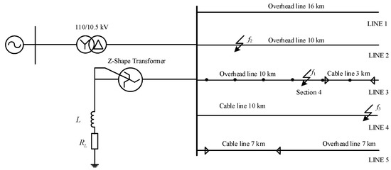
Figure 7.
Schematic diagram of single-phase grounding fault simulation of resonant grounding system.
The system was a 10 kV overhead-cable hybrid line distribution network, and the transformer transformation ratio was 110/10.5 kV. The load was three-phase balanced, the power was 1 MW, and the system frequency was 50 Hz. The system included five outgoing lines, of which line 4 was a pure cable line, line 1 and line 2 were pure overhead lines, and the remainder of the lines were hybrid lines. The lengths of these five lines are 16 km, 10 km, 13 km, 10 km and 14 km. The line parameters are shown in Table 1.

Table 1.
Line parameters of the simulation model.
In Table 1, R0 and C0 and L0 are zero-sequence resistance, capacitance and inductance, respectively. R1, C1 and L1 are the positive sequence resistance, capacitance and inductance, respectively.
We selected lines 2, 3 and 4 for simulation under different fault conditions when a single-phase ground fault occurs at 0.04 s, and we selected phase A as the faulty phase. Among them, f1 was 7 km away from the busbar, f2 was 3 km away from the busbar and f3 was 11.5 km away from the busbar.
The compensation degree of the arc suppression coil was −10%, which indicated an overcompensation state, and the inductance L of the arc suppression coil was
In Equation (10), fN is the power frequency, and the value is 50 Hz; C0 is the zero-sequence capacitance of the line; v is the compensation degree; l is the total length of the line. is the sum of zero-sequence capacitances of all lines.
Since v = −10%, L = 0.643 H can be obtained from Equation (10).
The resistance of the arc suppression coil was approximately 2.5~5.0% of the inductance, and a value of 3% was adopted in this study.
3.2. Simulation Results and Analysis under Different Fault Conditions
In order to verify whether the method is affected by the neutral point transition resistance, the initial phase angle of the fault, the location of the fault point, white Gaussian noise and distributed generation, and the simulation results were grouped according to the principles of the control variables.
- (1)
- Different transition resistances
Assuming that, in the resonant grounding system, line 3 has a single-phase grounding fault at point f1, and the initial phase angle of the fault is 0°, then the effectiveness of the faulty section location method under different transition resistances is verified. Table 2 shows the fault location results after using FCM clustering to process the DTW distance of each section.
Table 2.
Location results under different transition resistances.
Table 2.
Location results under different transition resistances.
| Transition Resistance/Ω | Cluster Center | Membership Degree Matrix | Location Result |
|---|---|---|---|
| 0 | Section 4 | ||
| 10 | Section 4 | ||
| 100 | Section 4 | ||
| 1000 | Section 4 | ||
| 3000 | Section 4 | ||
| 5000 | Section 4 |
From the analysis of Table 2, it can be seen that with the increase in the transition resistance, the value of the cluster center decreases. When the transition resistance increases to 1000 Ω, by analyzing the membership degree matrix, it can be seen that Section 4 is a class of its own, the membership value is 1.00 and the criterion is still obvious. When the transition resistance reaches 5000 Ω, although the value of the cluster center decreases, the change in the membership degree in the membership degree matrix is small, which shows that the fault location can still be achieved in the case of high-resistance grounding.
- (2)
- Initial phase angle of different faults
Assuming that, in the resonant grounding system, line 3 has a single-phase grounding fault at point f1, and the transition resistance is 10 Ω, the effectiveness of the faulty section location method under different fault initial phase angles is verified. Table 3 shows the fault location results after using FCM clustering to process the DTW distance of each section.
Table 3.
Location results of different fault initial phase angles.
Table 3.
Location results of different fault initial phase angles.
| Fault Initial Phase Angle/° | Cluster Center | Membership Degree Matrix | Location Result |
|---|---|---|---|
| 0 | Section 4 | ||
| 30 | Section 4 | ||
| 45 | Section 4 | ||
| 60 | Section 4 | ||
| 90 | Section 4 |
From the analysis of Table 3, it can be found that as the initial phase angle of the fault increases from 0° to 90°, the membership value of the faulty section and the nonfaulty section changes little, the value corresponding to the faulty section is always in a class of its own and the faulty section can still be located.
- (3)
- Fault occurring at the end of the line
Assuming that, in the resonant grounding system, a single-phase grounding fault occurs on line 4 at point f3, then the effectiveness of the method for locating the faulty section in the case of line-end faults is verified. Table 4 shows the fault location results after using FCM clustering to process the DTW distance of each section.
Table 4.
Location results of line-end faults.
Table 4.
Location results of line-end faults.
| Transition Resistance/Ω | Fault Initial Phase Angle/° | Cluster Center | Membership Degree Matrix | Location Result |
|---|---|---|---|---|
| 10 | 0 | line end fault | ||
| 500 | 90 | line end fault |
For the case in which a single-phase-to-ground fault occurs at the end of the line, simulations were carried out for different transition resistance and initial fault angle conditions, respectively. It can be seen from the membership degree matrix in Table 4 that there are no data of their own kind in the membership degree matrix, so it is determined that the line end is faulty.
- (4)
- Influence of white Gaussian noise
Assuming that, in the resonant grounding system, a single-phase grounding fault occurs on line 3 at point f1, then the transition resistance is 10 Ω, and the initial phase angle of the fault is 0°. We can verify the effectiveness of the faulty section location method under the influence of Gaussian white noise. Table 5 shows the fault location results after using FCM clustering to process the DTW distance of each section.
Table 5.
Localization results under the influence of white Gaussian noise.
Table 5.
Localization results under the influence of white Gaussian noise.
| Signal-to-Noise Ratio/db | Cluster Center | Membership Degree Matrix | Location Result |
|---|---|---|---|
| 30 | Section 4 | ||
| 60 | Section 4 | ||
| 90 | Section 4 |
It can be seen from Table 5 that adding Gaussian white noise interference with signal-to-noise ratios of 30, 60 and 90 db has little effect on the membership values of the faulty section and nonfaulty section, and will not affect the accuracy of fault location.
- (5)
- Influence of distributed generation access
Considering the influence of distributed generation access on the relay protection of the distribution network [16], the simulation tested the positioning results in the case of distributed power supply access. We assumed that, in the resonant grounding system, a single-phase grounding fault occurs on line 3 at point f1, and the busbar and line 5 are, respectively, connected to distributed power sources. We could verify the effectiveness of the method for locating the faulty section when the distributed power source is connected to the distribution network. Table 6 shows the fault location results after using FCM clustering to process the DTW distance of each section.
Table 6.
Positioning results of distributed generation connected to distribution network.
Table 6.
Positioning results of distributed generation connected to distribution network.
| Transition Resistance/Ω | Fault Initial Phase Angle/° | Cluster Center | Membership Degree Matrix | Location Result |
|---|---|---|---|---|
| 0 | 0 | Section 4 | ||
| 10 | 30 | Section 4 | ||
| 50 | 45 | Section 4 | ||
| 100 | 60 | Section 4 | ||
| 500 | 90 | Section 4 |
It can be seen from Table 6 that in the case of distributed power supply access, with the change in the transition resistance and the initial phase angle of the fault, the membership value of the faulty section and the nonfaulty section does not change significantly. The data of the faulty section in the membership degree matrix are always in a class of their own, which can realize fault location.
3.3. Comparative Analysis with other Positioning Methods
In order to demonstrate the superiority of the method proposed in this paper, a comparison between this method and the correlation coefficient method, the grey correlation degree method and the empirical mode decomposition was performed.
In the resonant grounding system, a single-phase grounding fault occurs at point f2 of line 2, the initial phase angle is 90°, and the transition resistance is 500 Ω. The fault location results after using FCM clustering to process the DTW distance of each section are shown in Table 7.
Table 7.
Comparison with other positioning methods.
Through the analysis of Table 7, it can be seen that under extreme working conditions, although the correlation coefficient method and the grey correlation degree method can locate the fault section, the criterion is not obvious. Using the empirical mode decomposition method to locate the fault, the difference between the adjacent energy weight coefficients of Section 2 and Section 4 is positive, and the criterion is invalid. However, the method proposed in this paper can still locate accurately under extreme fault conditions, and the criterion is obvious.
3.4. Field Data Test and Analysis
In order to confirm the effect of the method proposed in this paper, it was verified using the fault recording data. Two single-phase grounding faults occurred in a substation in a certain area, and the data recorded the zero-sequence currents of the four monitoring points of the faulty line, respectively. Figure 8 shows the fault zero-sequence current waveform plotted by MATLAB. The positioning results are shown in Table 8.
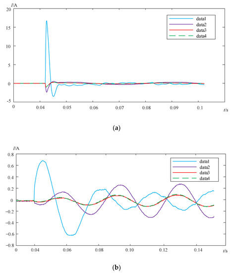
Figure 8.
Zero-sequence current waveform of each monitoring point of faulty line. (a) First fault data. (b) Second fault data.
Table 8.
The location results of field data test.
4. Conclusions
When a single-phase grounding fault occurs in the resonant grounding system, the transient zero-sequence current waveforms in the faulty section and the sound section are significantly different. In this paper, the transient zero-sequence current of each section of the faulty line is projected onto the transient zero-sequence voltage of the busbar, and the projected dynamic time warping (DTW) distance of each section is calculated. Finally, the DTW value of each section is classified by FCM clustering, and the membership degree matrix and cluster center are obtained. In the membership degree matrix, the section corresponding to the data in a class of their own is the faulty section, and all the other data correspond to the nonfaulty section. The conclusions are as follows:
- (1)
- The transient zero-sequence current of each section of the faulty line is projected onto the transient zero-sequence voltage of the busbar by the transient projection method, so that the difference between the faulty section and the nonfaulty section is more obvious, which can improve the location accuracy of single-phase grounding faults in resonant grounding systems.
- (2)
- The location method proposed in this paper can accurately locate a fault under the conditions of different transition resistances, different initial phase angles of faults and different fault points, and it has the ability to resist the interference of Gaussian white noise.
- (3)
- The positioning method proposed in this paper is also applicable to the case of distributed power access.
- (4)
- A large number of simulation data show that the positioning method proposed in this paper has strong adaptability to the high-resistance grounding fault in the resonant grounding system, reflecting that the transition resistance capability can reach 5000 Ω.
- (5)
- The method proposed in this paper is verified by the field data test.
In brief, the advantages of the method proposed in this paper are as follows:
- (1)
- No need to set threshold of fault location criterion.
- (2)
- Suitable for high resistance grounding fault.
- (3)
- Suitable for grid with distributed power access. Compared with steady-state positioning method, the transient positioning method proposed in this paper is relatively complex and requires higher data acquisition and processing capabilities of the positioning device.
Author Contributions
Conceptualization, Y.H. and X.Z.; software, R.W.; validation, M.C.; writing—original draft preparation, Z.G.; writing—review and editing, Z.Z.; visualization, W.Y. All authors have read and agreed to the published version of the manuscript.
Funding
This work was funded by the University and Zhangdian District Integration Development Project (2021JSCG0006).
Data Availability Statement
Not applicable.
Acknowledgments
The authors are very grateful to the anonymous referees for their helpful comments and constructive suggestions.
Conflicts of Interest
The authors declare no conflict of interest.
References
- Bingyin, X.; Yongduan, X.; Tianyou, L. Review of line selection of grounding fault in non-effectively grounding network techniques. Electr. Equip. 2005, 6, 1–7. [Google Scholar]
- Xue, Y.; Li, J.; Chen, X.; Xu, B.; Li, T. Faulty feeder selection and transition resistance identification of high impedance fault in a resonant grounding system using transient signals. In Proceedings of the CSEE, Savannah, GA, USA, 7–9 November 2017; Volume 37, pp. 5037–5048. [Google Scholar]
- Fang, Y.; Xue, Y.; Song, H.; Guan, T.; Yang, F.; Xu, B. Transient Energy Analysis and Faulty Feeder Identification Method of High Impedance Fault in the Resonant Grounding System. Proc. CSEE 2018, 38, 5636–5646. [Google Scholar]
- Ji, T.; Sun, T.J.; Xue, Y.D.; Xu, B.Y.; Chen, P. Current status and development of fault location technique for distribution network. Relay 2005, 33, 32–37. [Google Scholar]
- Zhensheng, W.U.; Xuechang, Y.A. Test on a transfer function algorithm for locating ground faults in power distribution networks. Autom. Electr. Power Syst. 2003, 27, 34–37. [Google Scholar]
- Huifen, Z.; Fan, Z.; Zhencun, P. Automatic fault locating algorithm based on signal injection method for distribution system. Electr. Power Autom. Equip. 2008, 28, 39–43. [Google Scholar]
- Zhang, L.; Wang, J.; Wang, L.; Jin, N.; Chen, M.; Jiang, W. A fault section location method for active distribution network based on discrete orthogonal S-transform and energy similarity. Electr. Meas. Instrum. 2019, 56, 50–55. [Google Scholar] [CrossRef]
- Yongduan, X.; Yining, S.; Riliang, L.; Bingyin, X.; Xiaoyong, Y. The processing technology of single-phase earth fault based on the transient power direction in non-solidly earthed network. Distrib. Util. 2018, 35, 3–8. [Google Scholar]
- Linli, Z.; Zhenzhen, G.; Shidong, Z. Location approach for single phase-to-earth fault in distribution network by comparing transient frequencies. Proc. CSU-EPSA 2017, 29, 135–138. [Google Scholar]
- Zheng, Q.; Tianqi, H.; Jianxiong, L. Analysis on grounding fault mechanism of DC filter in HVDC Transmission system. Autom. Electr. Power Syst. 2018, 42, 144–152. [Google Scholar]
- Weiguo, L.; Wenwen, X.; Zhenyu, Q. Fault location method of distribution network based on concave convex characteristics of transient zero sequence current. Power Syst. Prot. Control 2020, 48, 164–173. [Google Scholar] [CrossRef]
- Zhan, Q. Distribution Network High Impedance Fault Resolving Technique Study Based on Transition State Projection Method. Master’s Thesis, Fuzhou University, Fuzhou, China, 2018. [Google Scholar]
- Huang, C.; Liu, P.; Jiang, Y.; Leng, H.; Zhu, J. Line Differential Protection Based on Dynamic Time Warping Distance in Active Distribution Network. Trans. China Electrotech. Soc. 2017, 32, 240–247. (In Chinese) [Google Scholar]
- Penghui, L.I.; Chun, H. A fault section location method for small-current grounding fault in distribution network based on dynamic time warping distance. Power Syst. Technol. 2016, 40, 952–957. [Google Scholar]
- Shao, X.; Guo, M.; You, L. Faulty line selection method using mutual correlation cluster of grounding fault waveforms based on improved DTW method. Electr. Power Autom. Equip. 2018, 38, 63–71. [Google Scholar]
- Darioush, R.; Lu, T. A Literature Review of the Control Challenges of Distributed Energy Resources Based on Microgrids (MGs): Past, Present and Future. Energies 2022, 15, 4676. [Google Scholar] [CrossRef]
Publisher’s Note: MDPI stays neutral with regard to jurisdictional claims in published maps and institutional affiliations. |
© 2022 by the authors. Licensee MDPI, Basel, Switzerland. This article is an open access article distributed under the terms and conditions of the Creative Commons Attribution (CC BY) license (https://creativecommons.org/licenses/by/4.0/).