Article

Common Transmission Point (CTP) Gathers: A New Domain for Amplitude Variation with Offset

by
Lutfi Mulyadi Surachman
* and
Abdullatif Al-Shuhail
Department of Geosciences, King Fahd University of Petroleum & Minerals, Dhahran 31261, Saudi Arabia
*
Author to whom correspondence should be addressed.
Energies 2022, 15(13), 4825; https://doi.org/10.3390/en15134825
Submission received: 28 May 2022 / Revised: 19 June 2022 / Accepted: 23 June 2022 / Published: 1 July 2022
(This article belongs to the Section H3: Fossil)

Abstract

:
Analysis of amplitudes of transmitted waves (TAVO) is an extension of the conventional AVO analysis using amplitudes of reflected waves. In this study, we introduce the common transmission point (CTP) gather, which is a new domain that is convenient for TAVO analysis. A CTP gather is formed by binning traces that have the same transmission point across a layer interface. We use the proposed domain to invert the ratios Δ α α , Δ ρ ρ , Δ β β , and β α in a model consisting of a gas channel nestled within an oil reservoir. The TAVO equations are fitted to amplitudes calculated by Zoeppritz equations within CTPs inside and outside the channel. Within each CTP gather, we use all traces with incidence angles less than 90% of the critical angle (if any) as TAVO approximations break down beyond this point. The proposed CTP TAVO analysis method estimated Δ α α , Δ ρ ρ , Δ β β , and β α in the gas channel within 1% of their corresponding true values.

1. Introduction

Advances in the theory of waves involved the search for practical applications of Amplitude Variation with Offset (AVO), which started four decades ago. The behavior of elastic and light waves was speculated first by Green and Kelvin in the 1800s [1]. Knott in 1899 and Zoeppritz in 1919 used Snell’s law to derive generic expressions of shear and compressional wave reflections at a layer boundary due to changes in the velocities and/or densities of the layers in contact, which became the essential theoretical basis of AVO [2]. Eventually, the use of AVO in industrial applications such as hydrocarbon prospecting became widespread. Further development of the AVO application for hydrocarbon prospecting was reviewed by Foster in 2010 [3]. Selected reviews began with the work of Gregory in 1976 [4] and Domenico in 1977 [5], who discovered that pore fluid significantly affected the P- and S-wave velocity ratio, also known as Poisson’s ratio. A combined observation was made by Ostrander in 1984 that showed how the response of AVO reflection can be utilized to differentiate between the bright seismic amplitudes from nonhydrocarbon-bearing rocks such as basalt and those from gas sands. In this work, he showed that because of the contrast in the velocity difference between the gas sands and the surrounding rocks, at the far offset, many samples of gas sands caused reflections with jumped amplitudes [6].
In general, based on the geometry of seismic surveys, AVO analysis can be divided into conventional P-wave and converted P-SV wave analysis. For example, Goodway (2006) performed a conventional isotropic P-Wave AVO analysis in Calgary, Canada for mapping unconventional gas resources [7]. Effective pressure prediction using 4D seismic AVO data during CO2-EOR and storage was provided by Wang et al. (2020). This article separates the fluid pressure and saturation impact following CO2 injection using Landr’s time-lapse seismic AVO inversion approach. They differentiate the accuracy of Landr’s simplified formula with the AVO simplified equation of Gidlow and Smith that was used before Landr simplified the inversion of the pressure and saturations differences, concluding that the simplified formula of Gidlow and Smith was more accurate [8].
Zong et al. (2015) developed an equation of linearized P-Wave reflectivity in terms of fluid modulus to discriminate geofluids in the study of hydrogeology, geothermic, and exploration geophysics under general conditions [9].
Converted P-SV waves might generate a better signal-to-noise ratio because once propagated in rocks with unsaturated porosity, the attenuation of the S-wave is less than that of the P-wave [10,11,12]. Therefore, the analysis of converted wave AVO provides more information than the conventional P-wave analysis [13]. Gandomi et al. (2019) used specular imaging of converted wave data with the AVO impact. Application of the specular imaging approach to an ocean-bottom cable dataset from the North Sea resulted in a considerable increase in AVO yields [14]. Innanen (2012) use approximate expressions for converted AVO and AVF (amplitude variation with frequency) of a nonelastic target. It was found that 1/QS and 1/QP are proportional to the frequency rate of change of the reflection coefficients [15].
Converted reflected and downward transmitted waves were studied by Galperin et al. (2000). The study looked at how combining measurements from a horizontal and vertical profile allowed for the analysis of converted reflected waves and downward transmitted waves from the closest shot locations and included shallow depths. Converted downward transmitted waves linked with deeper interfaces were observed at larger distances. Converted upward transmitted waves with finely separated horizons arrived at the top region of the cross-section at the same time [16].
Donati and Martin (1998) presented the coefficient of RPS as a series of cosine and sine polynomials. They found that the sine polynomial approximation was more accurate up to a large angle of incidence than the cosine series approximation [17,18].
Ursin et al. (2020) showed that a curved contact changes the phase and amplitude of transmitted and reflected waves in anisotropic material. Seismic data recorded in complicated geological settings must be modified for geometrical spreading before doing analysis of amplitude-versus-angle/amplitude-versus-offset (AVA/AVO). The results of this study describe that the data should be corrected for the effects of interface by using ray theory to investigate the impact of reflector curvature and geometrical spreading on phase and amplitude changes for transmitted and reflected waves within anisotropic materials. An unusual scenario of homogeneous isotropic materials which are separated by a sloping interface was investigated in order to gain a better idea of the focusing effect of the contact [19].
Popoola et al. (2019) introduced the concept of transmission amplitude variation with offset (TAVO) by putting the Aki–Richards TPP approximation [20] in a Shuey-like form and expanding their TPS approximation in an odd-powered sine series [21]. They applied their method using receiver gathers while assuming a laterally homogeneous interface. In this study, we improve the TAVO method by introducing the common transmission point (CTP) gather, where only rays passing through the same transmission point are used for TAVO analysis.
The newly introduced CTP gather is analogous to a common midpoint (CMP) gather that is routinely used for conventional AVO analysis. Similar to a CMP gather, a CTP gather allows AVO analysis of transmitted waves in a vertical seismic profiling (VSP) survey without having to assume a laterally homogeneous interface (e.g., [20,21]).

2. Methodology

The approximate TPP and TPS expressions introduced by Popoola et al. (2019) are:
T PP ( θ ) = A + B tan 2 ( θ )
and
T PS ( θ ) [ C ] sin θ + [ D ] sin 3 ( θ ) + [ E ] sin 5 ( θ )
where:
A = ( 1 Δ ρ 2 ρ Δ α 2 α )
B = Δ α 2 α
C = β α ( Δ ρ ρ + 2 Δ β β ) + Δ ρ 2 ρ
D = β α ( ( Δ β β + Δ ρ 2 ρ ) β α ( 3 Δ ρ 4 ρ + 2 Δ β β ) )
E = 1 8 ( β α ( 2 Δ β β + Δ ρ ρ ) ( β α ) 4 ( 5 2 Δ ρ ρ + 8 Δ β β ) )
A list of all abbreviations is included in Abbreviations. Equations (3)–(7) can be inverted for the rock properties Δ α α , Δ ρ ρ , β α , and Δ β β as follows [18],
Δ α α = 2 B
Δ ρ ρ = 2 ( 1 ( A + B ) )
β α = C ( A + B + C 1 ) 2 D ( A + B 1 ) + A + B + C 1 A + B 1
Δ β β = ( A + B 1 ) ( 2 C ( A + B + C 1 ) 2 D ( A + B 1 ) + A + B + C 1 ) 2 ( C ( A + B + C 1 ) 2 D ( A + B 1 ) + A + B + C 1 )

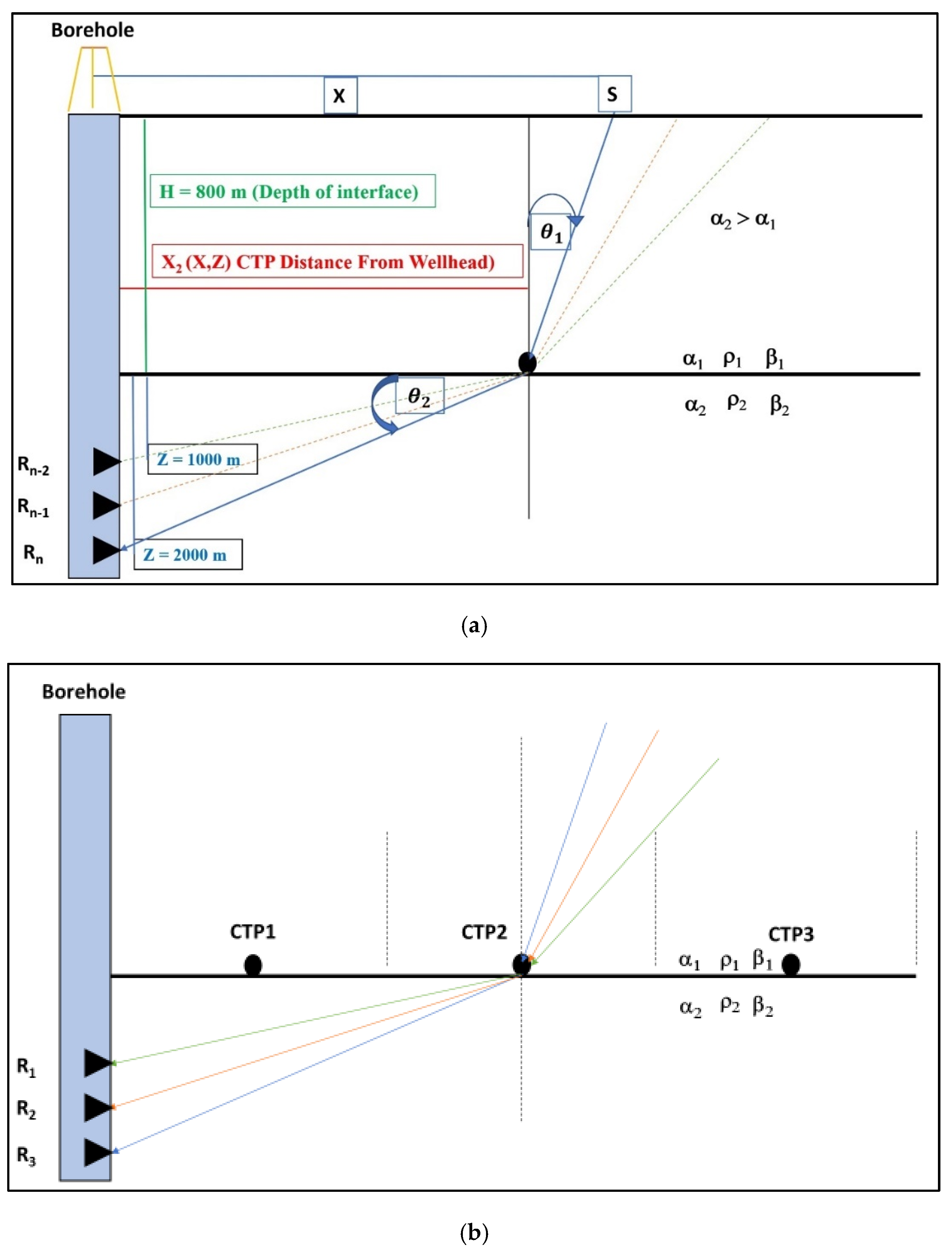
3. Common Transmission Point (CTP) Gather

Figure 1a shows a typical VSP geometry used to explain the CTP gather. A detailed derivation of the offset-angle transformation is given in Popoola et al. (2019). The distance of a transmission point of a ray from the wellhead (X2) is given by the following relation:
X 2 = ( Z H ) [ ( α 2 α 1 ) sin θ 1 1 ( α 2 α 1 ) 2 sin 2   θ 1 ]
The relationship between the incident angle and offset can be obtained generally by an equation derived by Popoola et al. (2019). For the models used in this study, the following fit is used [18]:
θ 1 = 0.0122695 X 6.73194 10 7 X 2
where θ 1 is the incidence angle in radians and X is the offset (horizontal distance between shot position and wellhead). The transmission angle θ 2 is calculated using Snell’s law as:
sin θ 2 = α 2 α 1 sin θ 1
The angle θ is then calculated as the average of θ 1 and θ 2 (see Abbreviations). For models where α 1 < α 2 , the critical angle is calculated as:
θ c = sin 1 ( α 1 α 2 )
A common transmission point (CTP) gather (or bin) will encompass all traces corresponding to rays transmitted within half shot spacing centered around that CTP (i.e., X2(X,Z) = xtpx in the Appendix A). The following workflow was used to generate the CTP gathers from the VSP data:
  • Use Equations (12)–(14) as well as the trace headers (i.e., survey geometry information) to calculate X2, θ 1, θ 2, and θ for every trace.
  • Group traces based on their X2 value lying within a length on the interface equal to one half of the shot spacing. Each of these groups constitutes one CTP gather.
  • Use Equation (15) to calculate the critical angle ( θ c) value for models where α 1 < α 2 .
  • Sort the traces in every CTP gather according to their θ value in increasing order from the trace with the minimum θ value available in that gather until the trace with θ value is less than or equal to (0.9 × θ c). If no critical angle exists, then, all traces of that gather are used.
  • Pick the times and amplitudes of the direct (down going) PP (i.e., TPP) and PS (i.e., TPS) waves on each trace of the CTP gather.
To apply TAVO analysis on a single CTP gather, the following workflow is used:
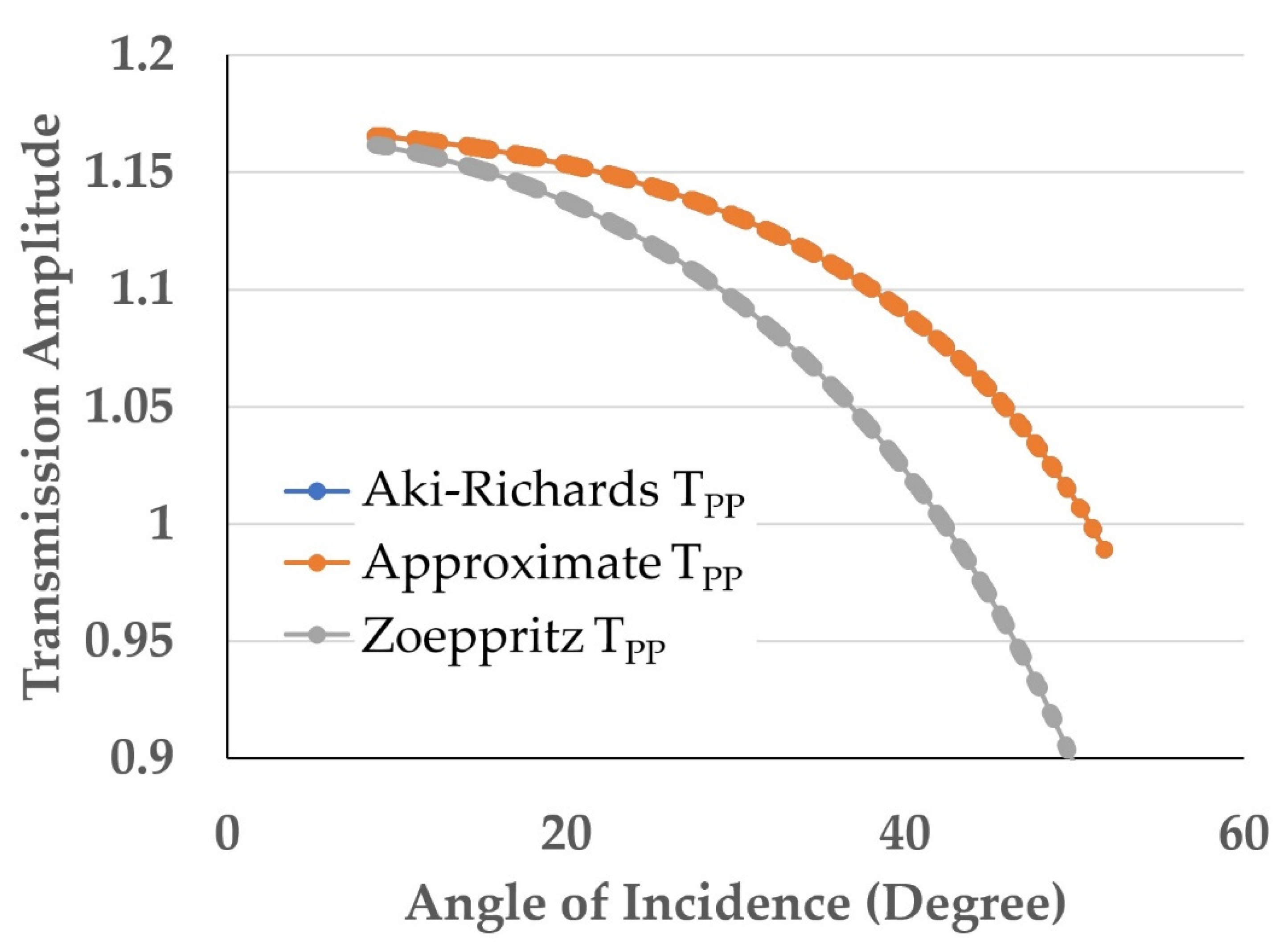
  • For every trace of the CTP gather, plot the picked TPP values versus their corresponding tan 2 θ values.
  • Fit a line to the ( tan 2 θ , TPP) data set. The intercept and gradient of this best-fit line are equal to A and B, respectively.
  • Use Equations (8) and (9) to calculate the rock properties Δ α α and Δ ρ ρ at the position of this CTP gather.
  • For every trace of the CTP gather, calculate sin θ .
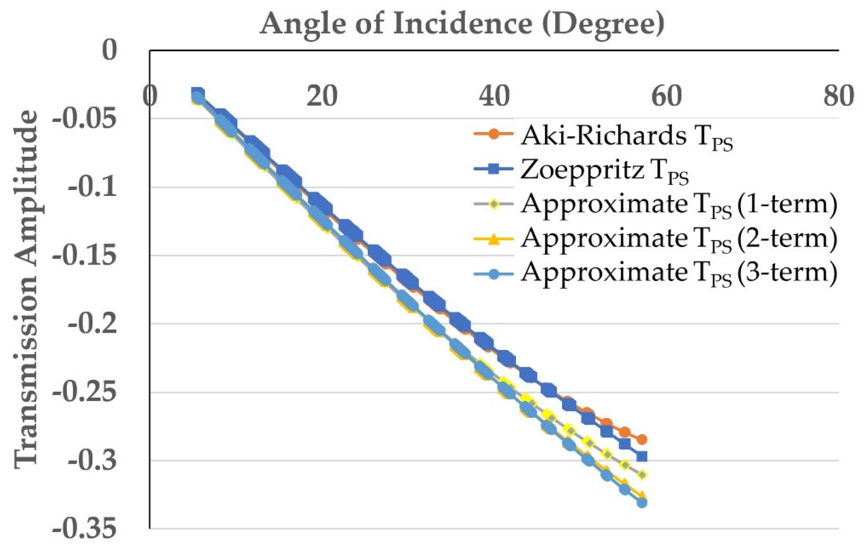
  • For a one-term approximation of the TPS, fit a line with zero intercept (i.e., f(x) = a1 x) to the ( sin θ , TPS) data set. The slope of this line is equal to C (i.e., C = a1)
  • For a two-term approximation of the TPS, fit a polynomial of the form f(x) = a2 x + b2 x3 to the ( sin θ , TPS) data set. Then, C = a2 and D = b2.
  • For a three-term approximation of the TPS, fit a polynomial of the form f(x) = a3 x + b3 x3 + c3 x5 to the ( sin θ , TPS) data set. Then, C = a3 and D = b3.
  • Use Equations (10) and (11) to calculate the rock properties β α and Δ β β at the position of this CTP gather.

4. Results and Discussion

We used the gas channel model shown in Figure 2 to test the performance of the CTP-TAVO analysis in estimating the properties of the gas channel. Table 1 provides the properties of the gas channel model formed from two models from Donati and Martin (1998).
Synthetic shot gathers were generated by the acquisition parameters in Table 2. The shot gathers were then sorted into CTPs and subsurface parameters were estimated using the procedures described in the previous section. The results for each CTP are described next.

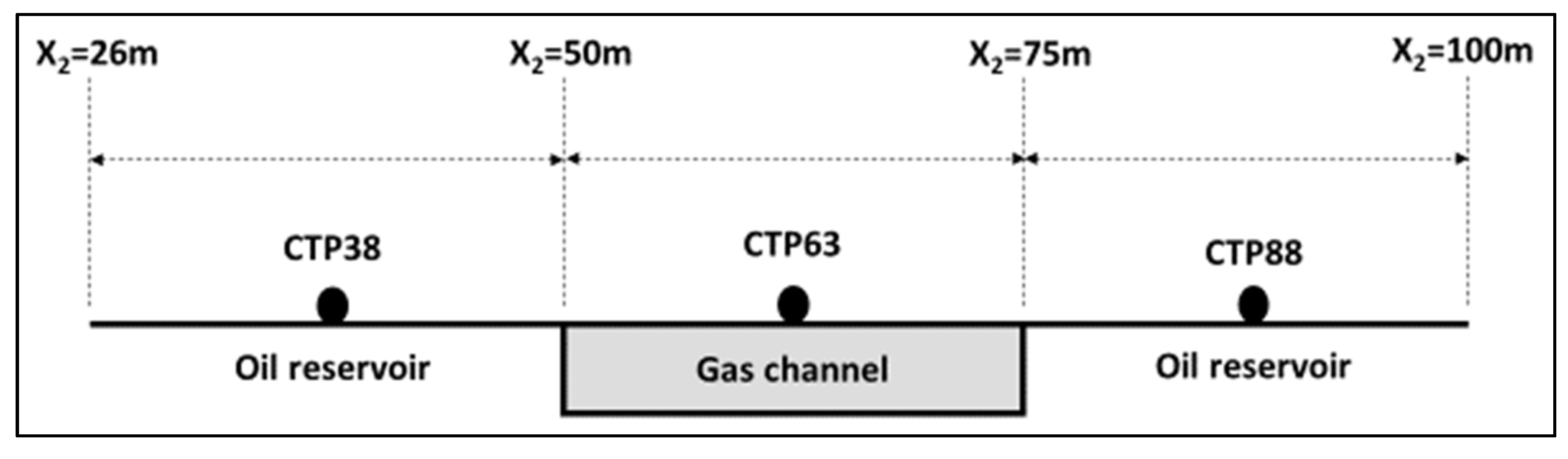
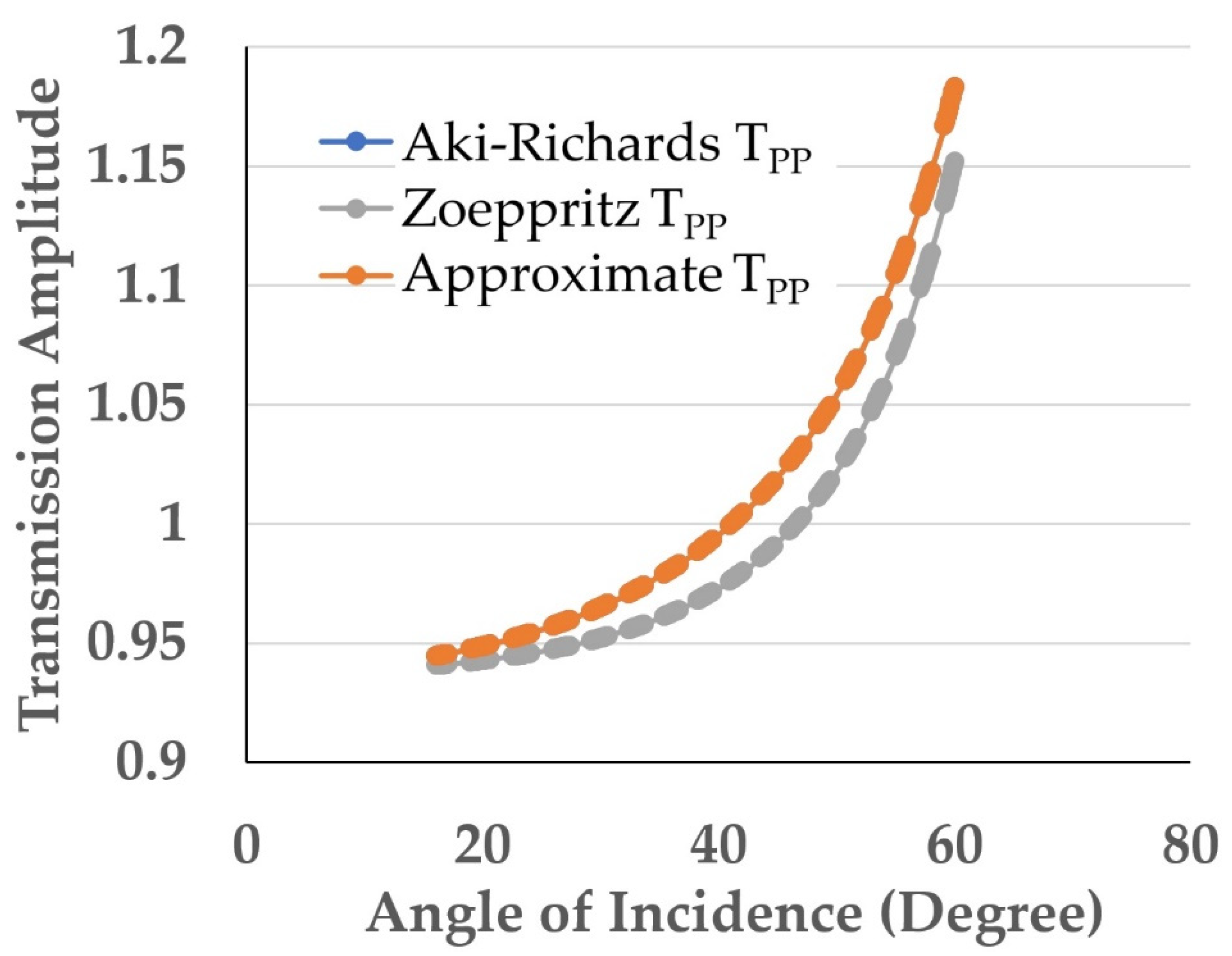
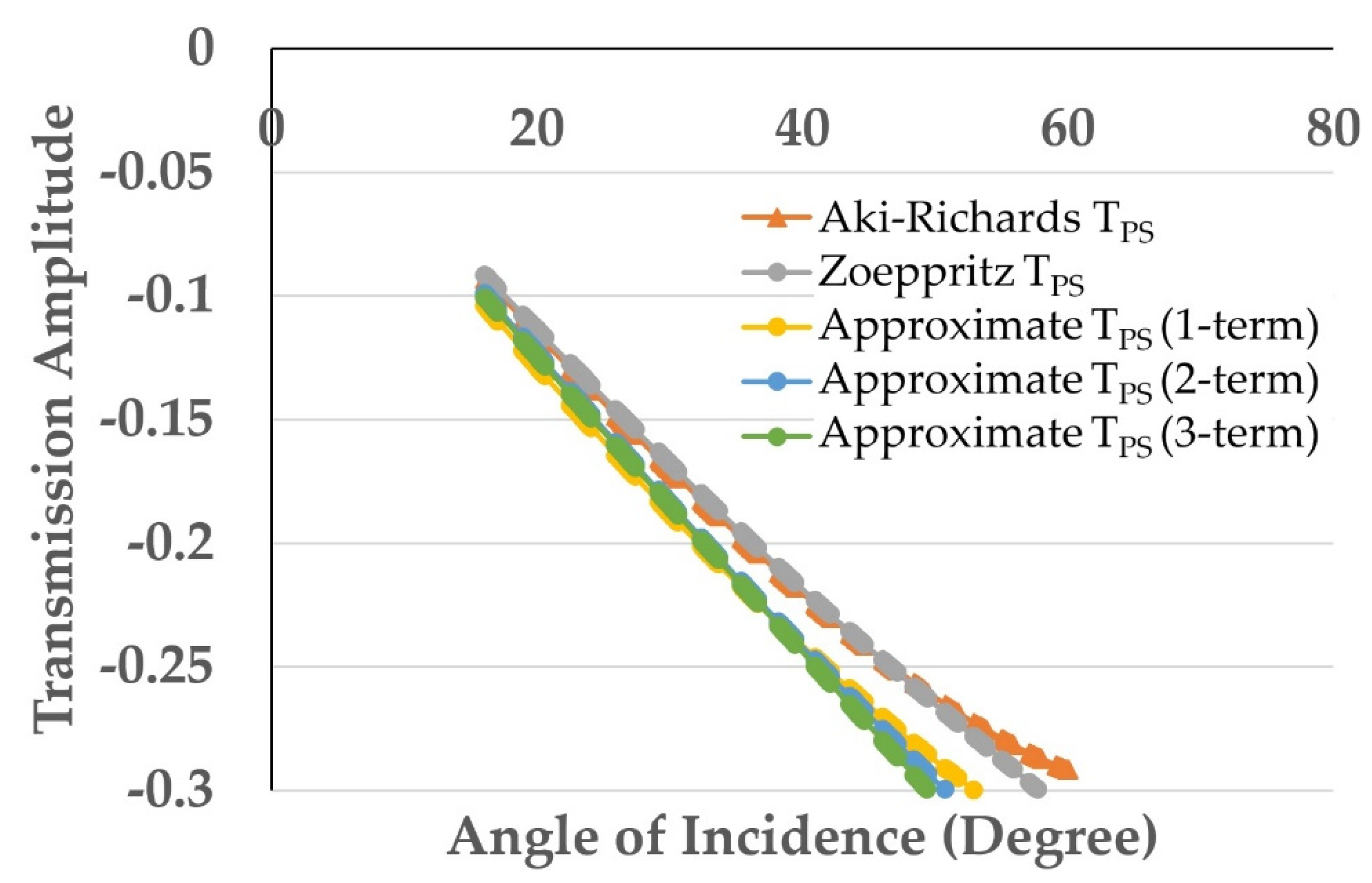
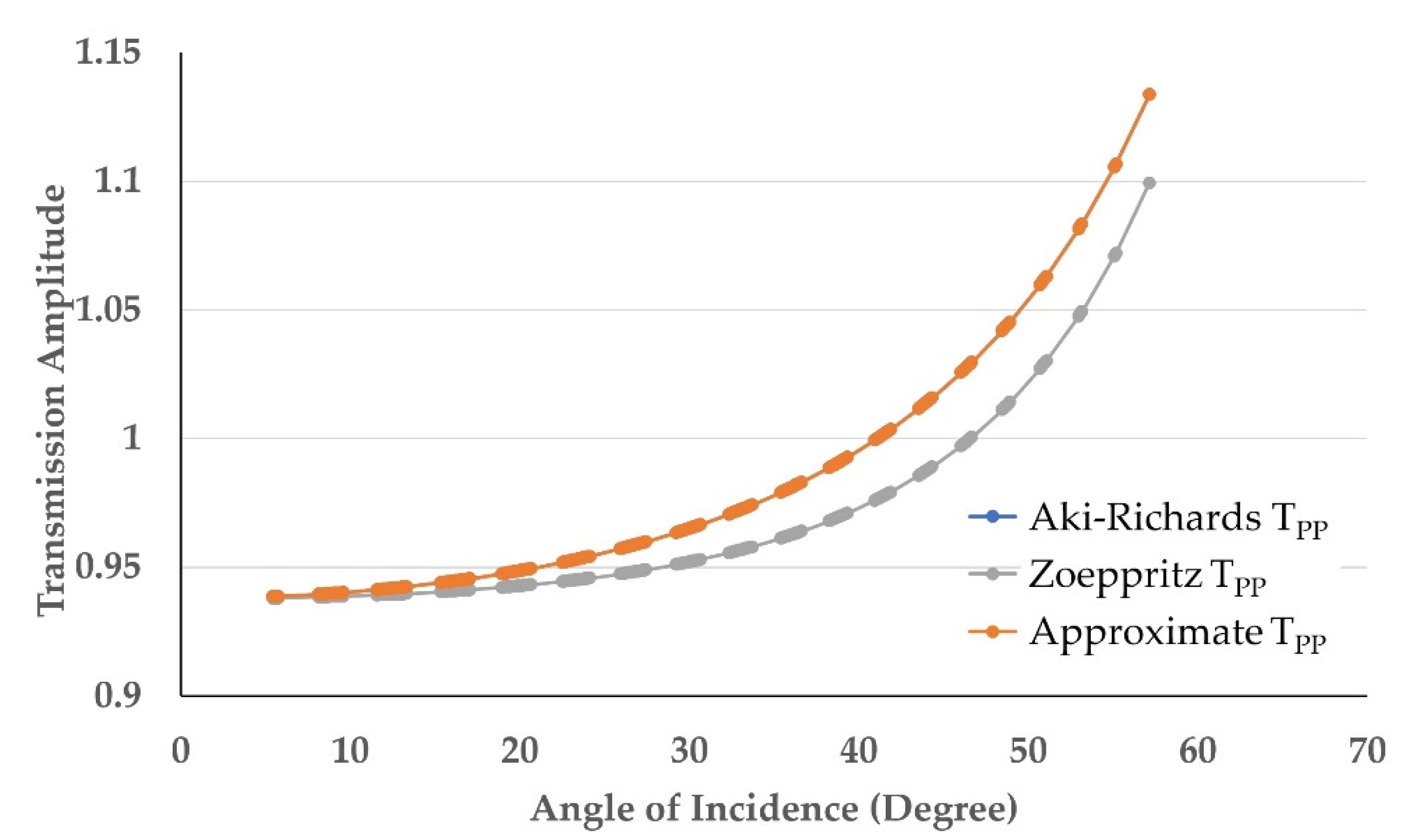
4.1. CTP Gather 26–50 m (CTP 38)

Figure 3 and Figure 4 show plots of TPP and TPS as a function of incident angle for a CTP 38 within the oil reservoir. Based on Figure 3, we can see that the Zoeppritz TPP and Aki–Richards approximations are coincident, while the approximate TPP slightly overestimates the Zoeppritz and Aki–Richards curves. Figure 4 shows the fits of Equation (2) using one, two, and three terms to the TPS angle–amplitude data of this CTP. We also plotted the TPS Aki–Richards approximation and exact Zoeppritz curve in the same figure for comparison. Regardless of the number of terms, all our approximations slightly underestimated both the Aki–Richards approximation and the exact Zoeppritz curve. The values of the fitting parameters (A, B, C, and D) are listed in Table 3. The subsurface parameters Δ α α , Δ ρ ρ , Δ β β , and β α inverted from these fitting parameters at this CTP are listed in Table 4, together with a comparison to their true values calculated from the model parameters.
The estimated values of Δ α α and Δ ρ ρ contained no error from the true values because their corresponding equations did not involve any approximation of Aki–Richards. However, the estimated values of Δ β β and β α involved errors (i.e., 0.58% and 7.8%, respectively) in this nearest CTP gather. One reason for the higher errors involved with this nearest offset CTP gather compared to the middle one might be due to approaching the critical angle, at which our approximations break down.

4.2. CTP Gather 51–75 m (CTP 63)

Figure 5 and Figure 6 show the plots of TPP and TPS as a function of the incident angle for CTP 63, which lies within the gas channel. Based on Figure 5, the Zoeppritz TPP and its Aki–Richard approximations are also coincident, while the approximate TPP curve also slightly overestimate both curves. Figure 6 shows the fits of Equation (2) using one, two, and three terms to the TPS angle–amplitude data of this CTP. We also plotted the TPS Aki–Richard approximation and exact Zoeppritz curve in the same figure for comparison. Regardless of the number of terms, all our approximations slightly overestimate both the Aki–Richards approximation and the exact Zoeppritz curve. The values of fitting parameters are listed in Table 5. The subsurface parameters Δ α α , Δ ρ ρ , Δ β β , and β α inverted from these fitting parameters at this CTP are listed in Table 6, together with a comparison to their true values calculated from the model parameters.
Similar to CTP 38, the estimated values of Δ α α and Δ ρ ρ contained no error from the true values for the same reasons. Moreover, the estimated value of Δ β β involved an error of 0.62%, which is close to that encountered in CTP 38 (0.58%). In comparison, the estimated value of β α involved an error of only 0.23%, which is much less than the error encountered in CTP 38 (7.8%). Compared to the other two CTP gathers, this CTP has similar or less errors in estimating the subsurface parameters Δ α α , Δ ρ ρ , Δ β β , and β α . One reason for less errors involved with this CTP might be attributed to the absence of a critical angle due to velocity inversion across the interface, which causes our approximations to deteriorate.

4.3. CTP Gather 76–100 m (CTP 88)

Figure 7 and Figure 8 show the plots of TPP and TPS as a function of incident angle for the CTP of 88 within the oil reservoir. Similar to the CTP of 38, the Zoeppritz TPP and Aki–Richards approximations are coincident, while the approximate TPP slightly overestimates both curves. Figure 8 shows the fits of Equation (2) using one, two, and three terms to the TPS angle–amplitude data of this CTP. We also plot the TPS Aki–Richards approximation and exact Zoeppritz curve in the same figure for comparison. Regardless of the number of terms, all our approximations slightly underestimate both the Aki–Richards approximation and the exact Zoeppritz curve. The values of the fitting parameters (A, B, C, and D) are listed in Table 7. The subsurface parameters Δ α α , Δ ρ ρ , Δ β β , and β α inverted from these fitting parameters at this CTP are listed in Table 8, together with a comparison to their true values calculated from the model parameters.
In this CTP, the estimated values of Δ α α and Δ ρ ρ also had no errors from the true values for the same reasons mentioned for CTP 38 above. However, the estimated value of Δ β β involved much higher error (6.33%) than errors encountered in CTP gathers 38 and 63. Similarly, the estimated value of β α involved much higher error (13.79%) than the errors encountered in CTP gathers 38 and 63. Moreover, the existence of a critical angle in this CTP (compared to CTP 63) causing our approximations to break down, the limited coverage of incidence angles (15–52°) in this CTP amplified the errors in estimating Δ β β and β α compared to CTP 38 that had a wider coverage of incidence angles (5–57°).

5. Conclusions

In conclusion, a new sorting domain (common transmission point) was introduced, which is suitable for AVO analysis of VSP data. Testing the new domain to estimate subsurface parameters in synthetic seismic data involving a gas channel within an oil reservoir showed that it is particularly effective in inverting gas channel properties. Although oil reservoirs are important to explore, a major target of AVO analysis are gas channels.
The proposed TPP expression offers accurate inversion results within Aki–Richards assumptions of small property contrasts across the interface and no angles close to 90° are involved. In comparison, the accuracy of the proposed TPS expression generally deteriorates near the critical angle and when using incidence angles that do not span both near and far offsets. In addition, geological and recording conditions of the real data may adversely affect the proposed TAVO analysis.
This work successfully developed the CTP concept and demonstrated it on synthetic data. Further work will involve attempting to obtain suitable, real VSP data for testing the proposed approach. Furthermore, development of this work to address anisotropy and viscoelastic effects is also planned.

Author Contributions

Conceptualization, A.A.-S.; methodology, A.A.-S.; software, A.A.-S. and L.M.S.; validation, A.A.-S. and L.M.S.; formal analysis, A.A.-S. and L.M.S.; investigation, A.A.-S. and L.M.S.; resources, A.A.-S.; data curation, A.A.-S. and L.M.S.; writing—original draft preparation, A.A.-S. and L.M.S.; writing—review and editing, A.A.-S. and L.M.S.; visualization, A.A.-S. and L.M.S.; supervision, A.A.-S.; project administration, A.A.-S.; funding acquisition, A.A.-S. All authors have read and agreed to the published version of the manuscript.

Funding

This research received no external funding.

Data Availability Statement

Data of this research are publicly available at: https://doi.org/10.6084/m9.figshare.20152952.

Acknowledgments

The authors would like to thank King Fahd University of Petroleum and Minerals for its support of this research under College of Petroleum Engineering and Geosciences startup fund project number 18060.

Conflicts of Interest

The authors declare no conflict of interest.

Abbreviations

α = α 1 + α 2 2 P-Wave average velocity
β = β 1 + β 2 2 S-Wave average velocity
Δ β = β 2 β 1 S-Wave velocity contrast
Δ α = α 2 α 1 P-Wave velocity contrast
Δ ρ = ρ 2 ρ 1 Density contrast
ρ = ρ 1 + ρ 2 2 Average density
θ = θ 1 + θ 2 2 Average incidence angle
RPPPP-reflection coefficient
RPSPS-reflection coefficient
TPSPS-transmission coefficient
TPPPP-transmission coefficient
CRGCommon receiver gather
VSPVertical seismic profiling
TAVOTransmission AVO

Appendix A. Mathematica and Phyton Codes to Obtain the Common Transmission Points

  • In [294]: = sxmin = 0.; (*min. offset of source*)
  • ns = 61; (*no. sources*)
  • dsx = 50.; (*increment of offset of source*)
  • rzmin = 1000.; (*min. depth of receivers*)
  • n = 101; (*no. receivers*)
  • drz = 10.; (*increment of depth of receivers*)
  • h = 800.; (*layer thickness*)
  • a1 = 3170.; (*P-wave velocity in layer 1*)
  • a2 = 3734.; (*P-wave velocity in layer 2*)
  • In [303]: = theta =
  • 0.0122695*. x - 6.73194 × 10^(-7) * x^2 (*x-theta relation - theta in degrees*)
  • Out [303] = 0.0122695x - 6.73194 × 10^(-7) x^2
  • In [305]: = txr = Pi/180.* theta (*theta in radians*)
  • Out [305] = 0.0174533 (0.0122695 x - 6.73194 × 10^-7 x^2)
  • In [307]: = xtpx = (z – h) * ((a2)/a1) * Sin[txr])/ Sqrt [1 – ((a2/a1) * Sin[txr])^2]
  • Out [307] =
  • 1.17792(-800.+. z) Sin[0.0174533 (0.0122695 x - 6.73194 × 10^−7 x^2)]/
  • Sqrt(1 - 1.38749 Sin[0.0174533(0.0122695 x - 6.73194 × 10^−7 x^2)]^2)
  • In [312]: = xzxtp = Flatten[Table[{(j − 1) * dsx + sxmin, (i − 1) * drz + rzmin,
  • xtpx/. {x -> (j − 1) * dsx + sxmin, z → (i − 1) * drz + rzmin}}, {j, 61}, {i, 101}],
  • 1](*. All possible transmission points*)
  • Out [312] =
  • {0., 1000., 0.}, {0., 1010., 0.}, {0., 1020., 0.}, {0., 1030., 0.},
  • {0., 1040., 0.}, {0., 1050., 0.}, {0., 1060., 0.}, {0., 1070., 0.},
  • {0., 1080., 0.}, {0., 1090., 0.}, {0., 1100., 0.}, {0., 1110., 0.},
  • ⋯6138⋯, {3000., 1900., 829.864}, {3000., 1910., 837.409},
  • {3000., 1920., 844.953}, {3000., 1930., 852.497}, {3000., 1940., 860.041},
  • {3000., 1950., 867.586}, {3000., 1960., 875.13}, {3000., 1970., 882.674},
  • {3000., 1980., 890.218}, {3000., 1990., 897.762}, {3000., 2000., 905.307}
  • large output show less show more show all set size limit...
  • In [313]: = Export[“xzxtp.xlsx”, xzxtp]
  • Out [313] = xzxtp.xlsx
# -*- Phytons code to sort xzxtp according to x2 and collect all rays in each 25m interval into one set *-
  • import pandas as pd
  • #import itertools
  • df = pd.read_excel(‘xzxtp.xlsx’)
  • X2_sorted = df.sort_values([“X2”, “Z”], ascending = True)
  • df1 = X2_sorted[(X2_sorted[‘X2’] >= 0) & (X2_sorted[‘X2’] <= 26)]
  • df2 = X2_sorted[(X2_sorted[‘X2’] >= 26) & (X2_sorted[‘X2’] <= 50)] -*CTP 38*-
  • df3 = X2_sorted[(X2_sorted[‘X2’] >= 51) & (X2_sorted[‘X2’] <= 75)] -*CTP 63*-
  • df4 = X2_sorted[(X2_sorted[‘X2’] >= 76) & (X2_sorted[‘X2’] <= 100)] -*CTP 88*-
  • df5 = X2_sorted[(X2_sorted[‘X2’] >= 101) & (X2_sorted[‘X2’] <= 125)]
  • df6 = X2_sorted[(X2_sorted[‘X2’] >= 126) & (X2_sorted[‘X2’] <= 150)]
  • df7 = X2_sorted[(X2_sorted[‘X2’] >= 151) & (X2_sorted[‘X2’] <= 175)]
  • df8 = X2_sorted[(X2_sorted[‘X2’] >= 176) & (X2_sorted[‘X2’] <= 200)]
  • df9 = X2_sorted[(X2_sorted[‘X2’] >= 200) & (X2_sorted[‘X2’] <= 225)]
  • df10 = X2_sorted[(X2_sorted[‘X2’] >= 226) & (X2_sorted[‘X2’] <= 250)]
  • df11 = X2_sorted[(X2_sorted[‘X2’] >= 251) & (X2_sorted[‘X2’] <= 275)]
  • df12 = X2_sorted[(X2_sorted[‘X2’] >= 276) & (X2_sorted[‘X2’] <= 300)]
  • df13 = X2_sorted[(X2_sorted[‘X2’] >= 301) & (X2_sorted[‘X2’] <= 325)]
  • df14 = X2_sorted[(X2_sorted[‘X2’] >= 326) & (X2_sorted[‘X2’] <= 350)]
  • df15 = X2_sorted[(X2_sorted[‘X2’] >= 351) & (X2_sorted[‘X2’] <= 375)]
  • df16 = X2_sorted[(X2_sorted[‘X2’] >= 376) & (X2_sorted[‘X2’] <= 400)]
  • df17 = X2_sorted[(X2_sorted[‘X2’] >= 401) & (X2_sorted[‘X2’] <= 425)]
  • df18 = X2_sorted[(X2_sorted[‘X2’] >= 426) & (X2_sorted[‘X2’] <= 450)]
  • df19 = X2_sorted[(X2_sorted[‘X2’] >= 451) & (X2_sorted[‘X2’] <= 475)]
  • df20 = X2_sorted[(X2_sorted[‘X2’] >= 476) & (X2_sorted[‘X2’] <= 500)]
  • df21 = X2_sorted[(X2_sorted[‘X2’] >= 501) & (X2_sorted[‘X2’] <= 525)]
  • df22 = X2_sorted[(X2_sorted[‘X2’] >= 526) & (X2_sorted[‘X2’] <= 550)]
  • df23 = X2_sorted[(X2_sorted[‘X2’] >= 551) & (X2_sorted[‘X2’] <= 575)]
  • df24 = X2_sorted[(X2_sorted[‘X2’] >= 576) & (X2_sorted[‘X2’] <= 600)]
  • df25 = X2_sorted[(X2_sorted[‘X2’] >= 601) & (X2_sorted[‘X2’] <= 625)]
  • df26 = X2_sorted[(X2_sorted[‘X2’] >= 626) & (X2_sorted[‘X2’] <= 650)]
  • df27 = X2_sorted[(X2_sorted[‘X2’] >= 651) & (X2_sorted[‘X2’] <= 675)]
  • df28 = X2_sorted[(X2_sorted[‘X2’] >= 676) & (X2_sorted[‘X2’] <= 700)]
  • df29 = X2_sorted[(X2_sorted[‘X2’] >= 701) & (X2_sorted[‘X2’] <= 725)]
  • df30 = X2_sorted[(X2_sorted[‘X2’] >= 726) & (X2_sorted[‘X2’] <= 750)]
  • df31 = X2_sorted[(X2_sorted[‘X2’] >= 751) & (X2_sorted[‘X2’] <= 775)]
  • df32 = X2_sorted[(X2_sorted[‘X2’] >= 776) & (X2_sorted[‘X2’] <= 800)]
  • df33 = X2_sorted[(X2_sorted[‘X2’] >= 801) & (X2_sorted[‘X2’] <= 825)]
  • df34 = X2_sorted[(X2_sorted[‘X2’] >= 826) & (X2_sorted[‘X2’] <= 850)]
  • df35 = X2_sorted[(X2_sorted[‘X2’] >= 851) & (X2_sorted[‘X2’] <= 875)]
  • df36 = X2_sorted[(X2_sorted[‘X2’] >= 876) & (X2_sorted[‘X2’] <= 900)]
  • df37 = pd.concat([d.reset_index(drop = True) for d in [df1, df2,df3,df4,df5,df6,df7,df8,df9,df10,df11,df12,df13,df14,df15,df16,df17,df18,df19,df20,df21,df22,df23,df24,df25,df26,df27,df28,df29,df30,df31,df32,df33,df34,df35,df36]], axis = 1)
  • df37.to_excel(‘xtpGrouping.xlsx’,index = False)

References

  1. Green, G. On the Laws of the Reflexion and Refraction of Light at the Common Surface of Two Noncrystallized Media; GeoScienceWorld: McLean, VA, USA, 2007. [Google Scholar]
  2. Knott, C.G., III. Reflexion and Refraction of Elastic Waves, with Seismological Applications. Lond. Edinb. Dublin Philos. Mag. J. Sci. 1899, 48, 64–97. [Google Scholar] [CrossRef] [Green Version]
  3. Foster, D.J.; Keys, R.G.; Lane, F.D. Interpretation of AVO Anomalies. Geophysics 2010, 75, 75A3–75A13. [Google Scholar] [CrossRef]
  4. Gregory, A.R. Fluid Saturation Effects on Dynamic Elastic Properties of Sedimentary Rocks. Geophysics 1976, 41, 895–921. [Google Scholar] [CrossRef]
  5. Domenico, S.N. Elastic Properties of Unconsolidated Porous Sand Reservoirs. Geophysics 1977, 42, 1339–1368. [Google Scholar] [CrossRef]
  6. Ostrander, W.J.T. Plane-Wave Reflection Coefficients for Gas Sands at Nonnormal Angles of Incidence. Geophysics 1984, 49, 1637–1648. [Google Scholar] [CrossRef]
  7. Goodway, B.; Perez, M.; Varsek, J.; Abaco, C. Seismic Petrophysics and Isotropic-Anisotropic AVO Methods for Unconventional Gas Exploration. Lead Edge 2010, 29, 1500–1508. [Google Scholar] [CrossRef]
  8. Wang, H.; Wang, Z.; Ma, J.; Li, L.; Wang, Y.; Tan, M.; Zhang, Y.; Cui, S.; Qu, Z. Effective Pressure Prediction from 4D Seismic AVO Data during CO2-EOR and Storage. Int. J. Greenh. Gas Control 2022, 113, 103525. [Google Scholar] [CrossRef]
  9. Zong, Z.; Yin, X.; Wu, G. Geofluid Discrimination Incorporating Poroelasticity and Seismic Reflection Inversion. Surv. Geophys. 2015, 36, 659–681. [Google Scholar] [CrossRef]
  10. Caldwell, J. Marine Multicomponent Seismology. Lead Edge 1999, 18, 1274–1282. [Google Scholar] [CrossRef]
  11. Mavko, G.; Mukerji, T.; Dvorkin, J. The Rock Physics Handbook; Cambridge University Press: Cambridge, UK, 2020. [Google Scholar]
  12. Thomsen, L. Converted-Wave Reflection Seismology over Inhomogeneous, Anisotropic Media. Geophysics 1999, 64, 678–690. [Google Scholar] [CrossRef] [Green Version]
  13. Sun, J.; Innanen, K. A Review of Converted Wave AVO Analysis. CREWES Res. Rep. 2014, 26, 1–13. [Google Scholar]
  14. JafarGandomi, A.; Bukola, O.; Refaat, R.; Hoeber, H. Specular Imaging of Converted Wave Data and Its AVO Impact. In Proceedings of the 81st EAGE Conference and Exhibition 2019, London, UK, 3–6 June 2019; European Association of Geoscientists & Engineers: Bunnik, The Netherlands, 2019; Volume 2019, pp. 1–5. [Google Scholar]
  15. Innanen, K.A. Anelastic P-Wave, S-Wave and Converted-Wave AVO Approximations. In Proceedings of the 74th EAGE Conference and Exhibition Incorporating EUROPEC 2012, Copenhagen, Denmark, 4–7 June 2012; European Association of Geoscientists & Engineers: Bunnik, The Netherlands, 2012; p. cp-293-00569. [Google Scholar]
  16. Gal’perin, E.I.; White, J.E. Vertical Seismic Profiling; Society of Exploration Geophysicists: Houston, TX, USA, 2000. [Google Scholar]
  17. Donati, M.; Martin, N.W. A Comparison of Approximations for the Converted-Wave Reflection. Techn. Rep. CREWES Res. Rep. 1998, 10, 16. [Google Scholar]
  18. Popoola, A.K.; Al-Shuhail, A.A.; Sanuade, O.A. Transmission Amplitude Variation with Offset (TAVO). J. Seism. Explor. 2019, 28, 413–424. [Google Scholar]
  19. Ursin, B.; Favretto-Cristini, N.; Cristini, P. Amplitude and Phase Changes for Reflected and Transmitted Waves from a Curved Interface in Anisotropic Media. Geophys. J. Int. 2021, 224, 719–737. [Google Scholar] [CrossRef]
  20. Aki, K.; Richards, P.G. Quantitative Seismology; University Science Books: Herndon, VA, USA, 2002. [Google Scholar]
  21. Al-Shuhail, A.A.; Popoola, A.K. Transmission Amplitude Variation with Offset (TAVO). In Proceedings of the Second EAGE Workshop on Borehole Geophysics, St. Julian’s, Malta, 21–24 April 2013; European Association of Geoscientists & Engineers: Bunnik, The Netherlands, 2013; p. cp-343-00042. [Google Scholar]
Figure 1. (a) CTP Configuration; (b) Several CTP bins with rays going through one of them.
Energies 15 04825 g001
Figure 2. Gas channel model used to test the CTP-TAVO analysis.
Energies 15 04825 g002
Figure 3. Fitting angle–amplitude (TPP) data of CTP 38 in the oil reservoir.
Energies 15 04825 g003
Figure 4. Fitting angle–amplitude (TPS) data of CTP 38 in the oil reservoir.
Energies 15 04825 g004
Figure 5. Fitting angle–amplitude (TPP) data of CTP 63 in the gas channel.
Energies 15 04825 g005
Figure 6. Fitting angle–amplitude (TPS) data of CTP 63 in the gas channel.
Energies 15 04825 g006
Figure 7. Fitting angle–amplitude (TPP) data of CTP 88 in the oil reservoir.
Energies 15 04825 g007
Figure 8. Fitting angle–amplitude (TPS) data of CTP 88 in the oil reservoir.
Energies 15 04825 g008
Table 1. Donati and Martin (1998) reported oil reservoir and gas channel models, respectively.
First LayerSecond Layer
Model α 1 (m/s) β 1 (m/s) ρ 1 (kg/m3) α 2 (m/s) β 2 (m/s) ρ 2 (kg/m3)
Oil reservoir317016982360373422792270
Gas channel304812452400243916302140
Table 2. VSP survey parameter simulation with the CTP configuration for the TAVO study.
ParameterValue
Top of reservoir (H)800 m
The first shot location (x,z)(0,0)
Shot spacing Δx50 m
Receiver depth1000–2000 m
Number of sources61
Maximum offset3000 m
Receiver spacing Δz10 m
Table 3. Values of the fitting parameters for CTP 38 in the oil reservoir.
Fitting ParameterValue
A0.937746672
B0.081691773
C−0.356696
D−0.0446039
Table 4. Subsurface parameter values and absolute errors for CTP 38 in the oil reservoir.
Subsurface ParameterTrue ValuesEstimated ValuesAbsolute Error (%)
Δ α α 0.1633835460.1633835460
Δ ρ ρ −0.03887689−0.038876890
Δ β β 0.2926093510.2909227940.58
β α 0.576187710.6211362767.8
Table 5. Values of fitting parameters for CTP 63 in the gas channel.
Fitting ParameterValue
A1.168071277
B−0.110802555
C−0.275596
D−0.0127772
Table 6. Subsurface parameter values and absolute errors for CTP 63 in the gas channel.
Subsurface ParameterTrue ValuesEstimated ValuesAbsolute Error (%)
Δ α α −0.22160511−0.221605110
Δ ρ ρ −0.114537445−0.1145374450
Δ β β 0.2677833140.2661179060.62
β α 0.5239100250.5226912410.23
Table 7. Values of fitting parameters for CTP 88 in the oil reservoir.
Fitting ParameterValue
A0.937746672
B0.081691773
C−0.353375
D−0.0561697
Table 8. Subsurface parameter values and absolute errors for CTP 88 in the oil reservoir.
Subsurface ParameterTrue ValuesEstimated ValuesAbsolute Error (%)
Δ α α 0.1633835460.1633835460
Δ ρ ρ −0.03887689−0.038876890
Δ β β 0.2926093510.274082996.33
β α 0.576187710.65569155313.79
Publisher’s Note: MDPI stays neutral with regard to jurisdictional claims in published maps and institutional affiliations.

