Article

Creating Comparability among European Neighbourhoods to Enable the Transition of District Energy Infrastructures towards Positive Energy Districts

1
Departamento Energías Renovables, Instituto Tecnológico de Canarias, Playa de Pozo Izquierdo s/n, 35119 Santa Lucía de Tirajana, Spain
2
Energy Economics Group, Technische Universität Wien, Karlsplatz 13, 1040 Vienna, Austria
3
Nottingham Business School, Nottingham Trent University, 50 Shakespeare Street, Nottingham NG1 4QU, UK
*
Author to whom correspondence should be addressed.
These authors contributed equally to this work.
Energies 2022, 15(13), 4720; https://doi.org/10.3390/en15134720
Submission received: 17 May 2022 / Revised: 13 June 2022 / Accepted: 18 June 2022 / Published: 28 June 2022
(This article belongs to the Special Issue Energy Consumption in a Smart City)

Abstract

:
Planning the required energy infrastructure for the energy transition is a crucial task for various neighbourhood concepts, such as positive energy districts. However, energy planning often comes with the challenges of data shortages and a lack of comparability among solutions for different districts. This work aims to enable this comparability by introducing an approach for categorising districts according to parameters that are relevant for the planning of neighbourhood energy infrastructures. Four parameters (climate, floor space index, heating demand and share of residential buildings) and their respective ranges (bands) were derived from the literature. Additionally, this work visualised the combination of all parameter bands across Europe to conveniently showcase districts that are comparable according to the selected parameters. This approach and its visualisation could be used in urban planning to share knowledge from existing energy district projects with those planned in comparable districts.

1. Introduction

Cities are responsible for about 70% of global C O 2 emissions, to which the largest contributor is the use of fossil fuels for buildings and transportation [1]. The concept of positive energy districts (PEDs), which are districts or neighbourhoods that have net-zero carbon emissions and positive annual energy balances, was proposed by the Strategic Energy Technology Plan (SET-Plan) Action 3.2 in 2018 as a cornerstone for the creation of carbon-neutral cities in Europe [2]. This action plan has led to various other initiatives across Europe (e.g., Making City [3], +cityXchange [4], IEA EBC Annex 83 (International Energy Agency’s Energy in Buildings and Communities programme) [5] and Pocityf [6]). In academia, PED-based research has also been increasing [7,8,9]. PEDs have been developed using different approaches and techniques from different actors. According to the Joint Programming Initiative (JPI) Urban Europe [10], there were two operating PEDs at the beginning of 2020, with 19 others in the implementation stage and 8 in the planning stage. Furthermore, 32 other projects have not declared ambitions to become PEDs but present characteristics of interest for PED development [10]. These projects span across Europe and provide cases for a wide variety of climates, political contexts, social contexts and national and local energy production mixes and infrastructure. These cases generate plenty of data that other local planners could potentially use for initial assessments and replications. In this context, comparability and replicability are crucial.
The transition towards positive energy districts needs appropriate infrastructure, as defined in Section 2. However, the kind of infrastructure and its capacity in terms of electricity or heating and cooling depend on characteristics that vary across Europe. For example, climate attributes, such as solar irradiation and temperature, affect the potential for photovoltaic (PV) generation, as well as heating and cooling systems. Many district energy system transformation projects rely on case studies for data specific to their locations [3,4,5,6]. However, it is not easy to know whether an analysis made for one area would apply to another area within the EU. Therefore, our work aimed to develop a methodology for classifying European districts based on parameters that are helpful in the initial evaluation and planning phase of energy infrastructures that could lead to PEDs.
The method developed in this study clusters existing neighbourhoods within Europe according to key categorisation parameters. This approach can provide benefits for both practice and theory. For example, categorising districts according to their energy infrastructure requirements is of practical use for regional decision-making in the initial stages of planning district energy infrastructures. It simplifies comparing solutions and approaches from other districts that fall into the same district category. The categorisation also supports learning from challenges and opportunities that arose from existing or studied areas, for example, in the planning stage. Furthermore, this categorisation could be of particular interest to academia within the field of energy modelling. The accessibility of data can be a significant burden for energy modelling-related research. Using the presented categorisation approach could justify using data relevant to the infrastructure requirements of another district with similar characteristics.
The remainder of the article begins by narrowing down the scope of the categorisation and introducing important background information in Section 2. Subsequently, Section 3 introduces the overall methodology of the work. The results are presented in Section 4, which also shows the procedure for identifying the relevant parameters for the district categorisation for infrastructure comparability, as well as their ranges (Section 4.1). This is followed by the application of this method to the creation of comparable districts using visualisation maps of different parameter combinations (Section 5). The work is finalised by an elaboration on the application, limitations and prospects of this method in Section 6.

2. Theoretical Background
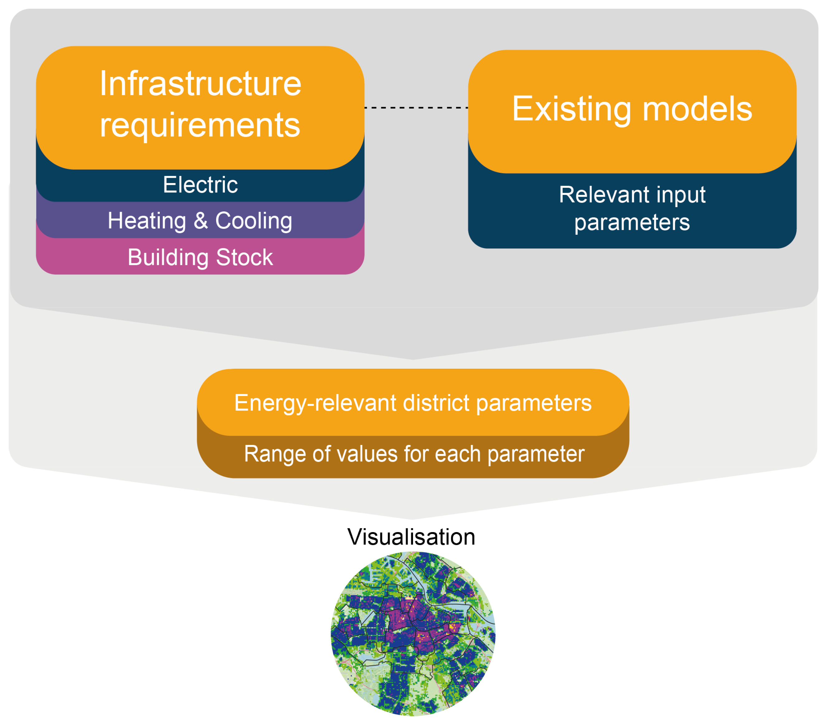
The positive energy goal, i.e., positive renewable annual energy balance, is barely achievable without the district energy infrastructures undergoing a major transformation [11]. Building on the works of Fulmer et al. [12] and Brozovsky et al. [13], this study defined a district energy infrastructure as the physical components of building and energy infrastructure systems (i.e., heating networks, electricity grids, generation, etc.) that provide commodities and services (e.g., hot water, electricity, etc.) that are essential for enabling, sustaining and enhancing societal living conditions.
According to JPI Urban Europe [2], each PED is supposed to find its own optimal balance between three main elements: the energy efficiency of the infrastructure, local renewable energy production and energy flexibility within the district (see Figure 1). These three elements are relevant to different parts of a district’s energy infrastructure, e.g., energy efficiency primarily relates to building envelopes and heating and cooling systems. Thermal insulation, more efficient decentralised boilers and district heating systems are crucial in colder climates. Buildings in warmer climates require insulation and ventilation to reduce cooling demands during hot summer periods. Once the energy efficiency limit is achieved, local energy supply from renewable sources, such as PV or wind power, is deployed to cover the local energy demands. Finally, the flexibility of an energy system can be provided by storage technologies and emerging services, such as dynamic charging for battery electric vehicles (BEV). Although this example has advanced and grown in importance over recent years, this work did not focus on BEVs and their charging. Smart charging and vehicle-to-grid technology are not yet widely implemented. Furthermore, readers can infer relevant information regarding mobility from some of the parameters selected for the classification efforts (Section 4), i.e., the residential share of the total gross floor area and the floor space index. Hence, necessary transformations are the measures (and their ambitions) that need to be implemented to achieve each “sub-goal” (i.e., element). For example, the “transformation” of a building envelope (e.g., insulating walls) or heating system (e.g., installing heat pumps) is necessary for energy efficiency, as energy efficiency is defined by the conditions or characteristics of those infrastructures.
Hence, for the purpose of this study, a PED infrastructure encompasses the following technology: renewable energy generation, energy storage, charging technology, building envelopes and heating and cooling systems. Each technology also has parametric and installed capacity requirements. Parametric requirements refer to, for example, the supply temperature needed for space heating. Finally, the installed capacity indicates the size of each system, e.g., the installed capacity of renewable generation technologies or the necessary capacity of district heating generation. Such parametric and capacity requirements are usually estimated using energy models [14].
Previously, several studies have attempted to analyse infrastructure requirements by creating district typologies. A German study presented a method for estimating infrastructure costs (for regional spatial planning) based on the structural type of the settlement [15]. Such typology-based approaches are based on the assumption that urban areas with similar building typologies and urban structures are similar in terms of infrastructure configurations and demands. Another approach for creating a district typology was proposed by [16] for estimating heat demands and thermal gains (and losses) within a district. The classification of districts was based on the building typologies and urban forms; thus, parameters such as building shape, district density and building age were used to categorise the districts. Other studies have not created archetypes but have instead analysed the urban characteristics of districts that could help create a sustainable neighbourhood [17,18]. As observed, district categorisation is highly dependent on the location; hence, it is usually not meant to be applied outside its original scope and region.

3. Methodology

This section presents the approach taken in this work to develop the district categorisation method, which was based on infrastructure requirements. This work incorporated three stages, as shown in Figure 2.
First, based on a critical review of the background literature, this work selected district-level energy models and identified the commonly used input parameters from those selected models. Appendix A shows the list of selected models, and information relevant to this study. The models covered the analysis and planning of the energy infrastructures, as discussed in Section 2. The next step was synthesising the findings to define the parameters for district categorisation according to energy infrastructures. Defining the approximate ranges of the values for each parameter was based on the relevant literature. Furthermore, this study showed that this conceptual method could be realised and applied in practice by extracting the raster layers of the defined parameters from Hotmaps, which is a validated open-source application for heating and cooling planning at various spatial levels [19,20,21]. These raster files of the parameters, which are essential for strategic heat planning, are estimated data. Hence, the limitations of these data should be taken into account (discussed further in Section 5). The Hotmaps data focus on residential buildings; therefore, using these data in non-residential areas must be performed with care. However, since PEDs are a highly residential concept, this limitation was justifiable. The Hotmaps data were further manipulated using the QGIS software. As a result, this study demonstrates similar districts across Europe that are likely comparable regarding infrastructure requirements. Figure 2 illustrates the overall methodology of our work.
The first stage of this work (Section 4.1) looked at the existing review papers that deal with models and tools that are used within the energy system modelling domain for various purposes. The article by [14] served as a starting point. The authors listed previous review articles that categorised or analysed energy system models and tools. Many review articles have focused on models that are suitable for analysing local-, community-, district- and neighbourhood-scale energy systems [22,23,24,25,26,27,28]. Hence, from the known models, we selected several models that comply with the following criteria, which we extrapolated from our energy infrastructure definition in Section 2:
(a)
A district or neighbourhood geographical scale (or any cluster of buildings);
(b)
A time resolution from hourly to seasonal;
(c)
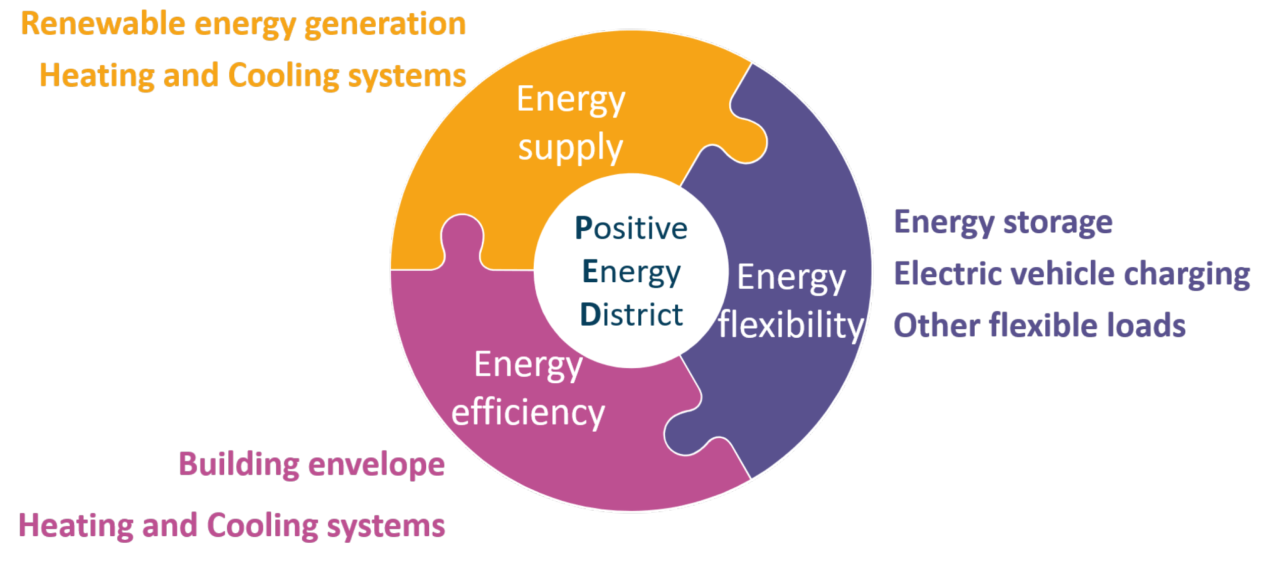
An infrastructure that was within the scope of this work, i.e., renewable energy generation technology, energy storage and EV charging technology, heating and cooling systems and building envelopes;
(d)
Aims that are relevant for energy planning (i.e., not frequency regulation or power sector specifics).
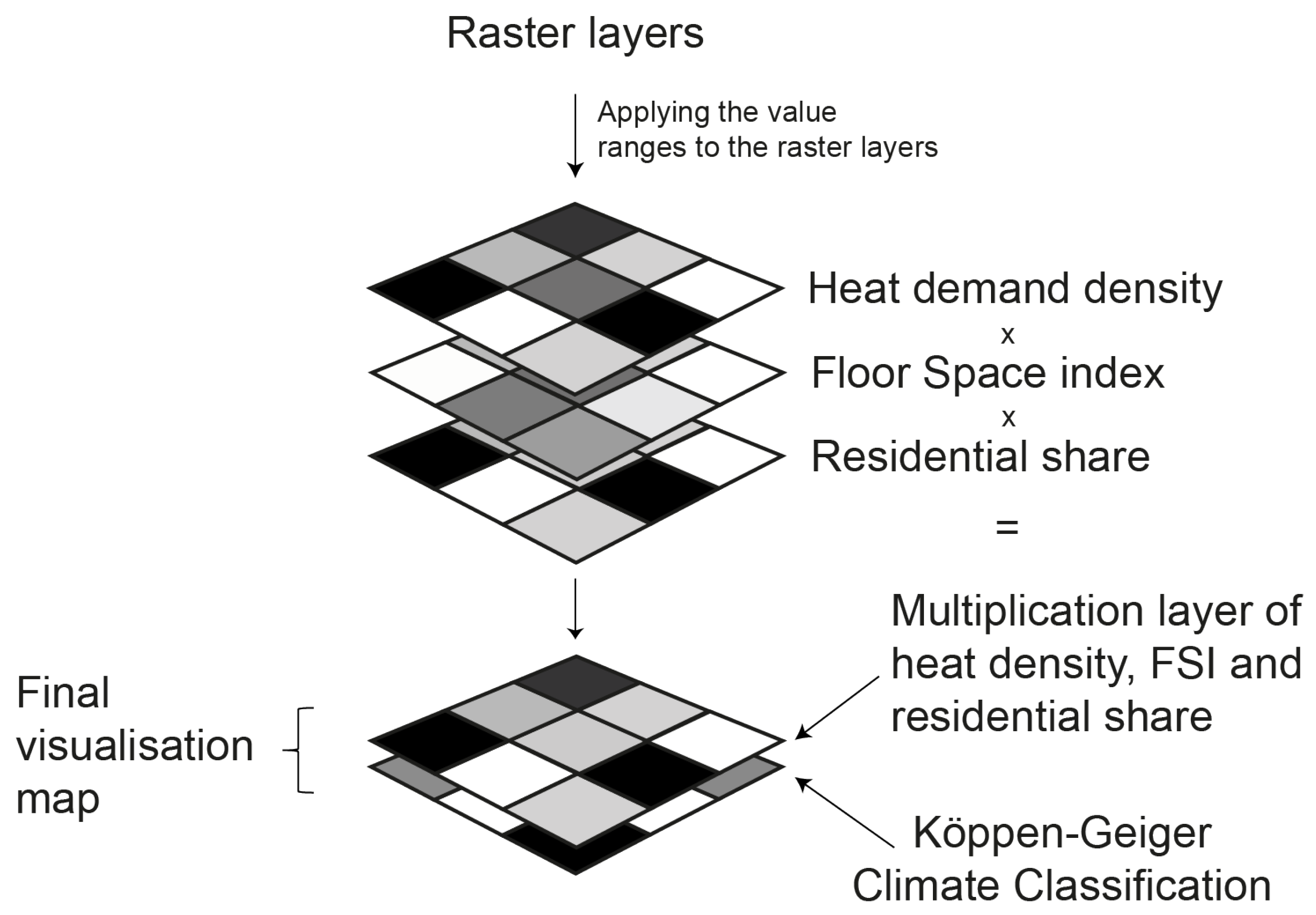
The next step after model selection was to summarise the information that was used as the inputs and outputs of the models, as well as the modelling approach (i.e., method), spatial and temporal scales and the covered infrastructure types. Then, we analysed and generalised the input parameters (along with the other information that was collected) to derive the parameters for our district categorisation (Section 4.1). As specific and granular data are not always available, using generalised district parameters could help with the research for and planning of PEDs (or other related district energy concepts). The extracted district categorisation matrix is illustrated in Section 5, which shows the district typologies that are present in Europe. The cities of Amsterdam, Frankfurt and Torres Vedras, along with selected districts, were used to showcase the use of the final parameter map. These cities were selected in line with the case study cities of the PED-focused “Smart-BEEjS” project. Furthermore, to adequately showcase the comparison map, two cities/districts within the same climate zone were needed (Frankfurt and Amsterdam).

4. Model Details

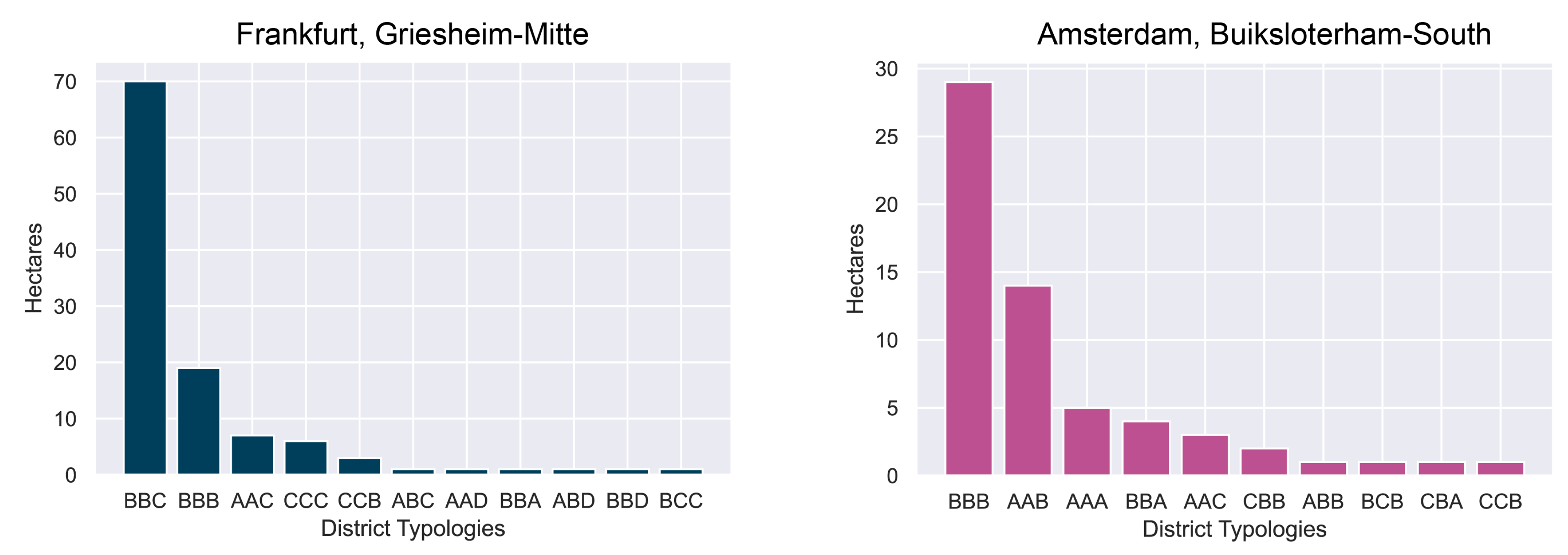
4.1. Input Parameters for District Categorisation

This study revised several district energy models with the aim of identifying their input requirements. The results of the review are presented in Table A1. These comprehensive and detailed input requirements were grouped into smaller sets of representative and comparable parameters that could be used to classify European neighbourhoods (Table 1). To achieve a feasible categorisation, four parameters that represent the most important input requirements were chosen. The summarised results of the energy modelling review, which are shown in Table 1, were in line with the literature research that was carried out by [29,30].
The “climate zone” parameter in Table 1 refers to meteorological and weather- and climate-related data. This input influences heat demands and renewable energy supplies and, therefore, is crucial for the selection of local energy infrastructures. The most widely used climate classification is the Köppen–Geiger (KG) classification [31], which divides the world into five regions and 30 sub-regions according to the threshold values and seasonality of monthly air temperature and precipitation [32]. This classification scheme has been used in the PV community to analyse regions of interest easily [33]. For example, the European project PVSites applied the Köppen–Geiger classification, together with the parameters of the European heat index and European cooling index, to create a zoning map for nearly zero energy buildings (nZEBs) [34].
The “heating demand” parameter indicates the levels of demand for space heating in buildings, which mainly depends on the climate and the energy efficiency state of the buildings. The values and ranges for the annual heat demand were identified from the available data, as explained further in Section 5. This parameter mainly influences the building envelopes and heating and cooling systems.
The “floor space index” parameter ( F S I ) can also be an indication of the space that is available for renewable energy generation in relation to the number of people living and consuming energy in that specific area, as described by [35]. The F S I (also called the floor area ratio) is defined by Equation (1) [36]:
F S I = g r o s s f l o o r a r e a p l o t a r e a
The F S I ranges indicate the type of the settlements within a neighbourhood: very rural settlements (<0.25), single-family houses (0.25–1), row housing (1–2) and block housing to very dense urban settlements (>2) [35]. A lower F S I could indicate that a larger area (roofs) is available for renewable energy generation, while the overall energy demand density stays low. Thus, a low F S I indicates the increased technical ease of achieving the PED energy balance requirements. However, it does not indicate anything about economic aspects.
The “share of residential buildings” parameter is an indication of the type of energy consumer that is present in a neighbourhood. The type of consumer affects the final net energy consumption of building operations and the load distribution over time [37]. More specifically, the ratio of residential to commercial consumers influences the final net consumption of buildings, as commercial buildings have higher energy requirements (especially supermarkets) [37]. In addition, the electric load distribution of residential buildings is significantly different from that of non-residential buildings, with the residential load being higher during morning and evening hours [38]. Additionally, potential EV charging schedules also depend on the residential share of buildings, as cars are usually available for charging at night in residential districts and during working hours in non-residential districts.
All parameters are shown with their respective ranges in Figure 3. The ranges of the parameters were derived based on the available data, as described in Section 5.
The procedure for visualising of district types across Europe is illustrated in Figure 4. First, a raster file of each selected parameter (except for the climate zone parameter) was extracted from the Hotmaps library [20]. The raster layers had a resolution of one hectare; therefore, each hectare equalled one pixel of the raster layer and was associated with one relevant parameter value (e.g., heating demand). To limit the combination of possibilities, this study reduced the available values of the raster layers to our predefined ranges, according to Figure 3. The multiplication of all the Hotmaps-derived raster files resulted in one raster layer with a maximum number of n x possible district typologies, where n is the number of parameters and x is the number of values that each parameter could obtain. Furthermore, we imported a Köppen–Geiger climate raster file [32] of Europe and overlaid it on the output file (i.e., the district typology map). The climate layer was not multiplied with the remaining parameter layers as it would significantly increase the number of possible combinations that were available. Therefore, the climate layer functioned as an initial filter to find districts within the same climate zone before advancing with the remaining layers. The final two-layer map showed all available combinations of the heat demand, F S I and residential share parameters (as defined in Section 4) on one layer and the climate zone parameter on another layer. Therefore, the map enabled the easy comparison of different districts according to the predefined parameters.
Defining the parameter value ranges was essential to the categorisation effort. The number of bands had to be kept low to decrease the possible combinations of the values but high enough to guarantee sufficient detail. As the F S I was unavailable as a raster file, this study approximated it using the gross floor area per hectare. The heating demand and the F S I value distributions followed an F-distribution. Furthermore, the heating demand distribution was strictly related to the F S I ; thus, the quantiles of the F S I thresholds were transferred to the heat demand values, as defined in Section 4.1, to generate the thresholds that are shown in Figure 3. The residential share distribution showed two peaks on the left- and right-hand sides of the graph, with a valley in the middle. This distribution showed that the most common districts had either a low or high residential share of the gross floor area. Nonetheless, many districts still had a residential share between these two peaks. Applying the exact quantiles used for the F S I and heat demand parameters meant considering a large proportion of the districts to be highly residential, which distorted the categorisation efforts. Consequently, this work divided the residential share values into four equidistant bands. For the first three parameters in Figure 3 (heat demand, F S I and residential share), the letters A to D were used to classify the bands, with A being the lowest and D being the highest value. All of the prevalent climate zones in Europe, according to [32] were used. This work only included heating demand instead of additionally including the cooling demand. Arguably, across one climate zone and one F S I category, the heating demand and cooling demand would be negatively correlated, meaning that heating demand band A would correlate to cooling demand D and vice versa. Thus, adding this additional layer would have increased complexity without adding much additional value. The final district categorisation matrix with the selected parameters and their relevant bands is illustrated in Figure 3.
Figure 5 shows the general application process of the final district typology map (openly accessible). Firstly, two or more districts located in the same KG climate zone need to be chosen for the analysis. After using this climate filter, the climate map can then be disabled to only visualise the districts’ typology created by the heat demand density, the FSI and the residential share. The analysis of this can be visual or statistical by extracting the values of the raster layers belonging to each district. If the districts have similar typologies, a high potential for a similar approach towards energy infrastructure requirements can be deducted. Thus, districts that are very similar according to the defined parameters and fall into the same climate zone can initiate knowledge exchange within the planning teams. On the other hand, if the district typologies vary significantly, the potential for a similar approach is lower.

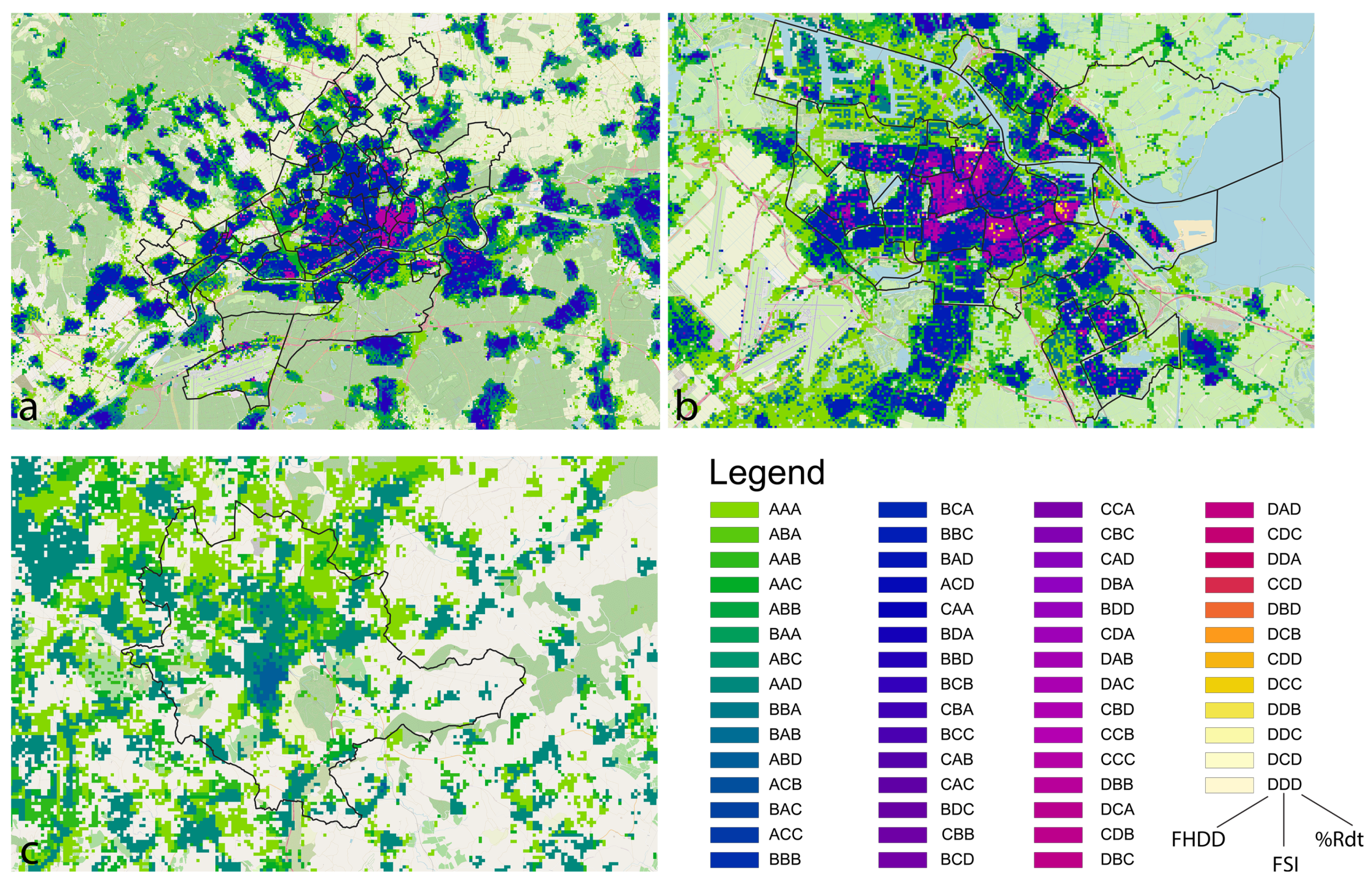
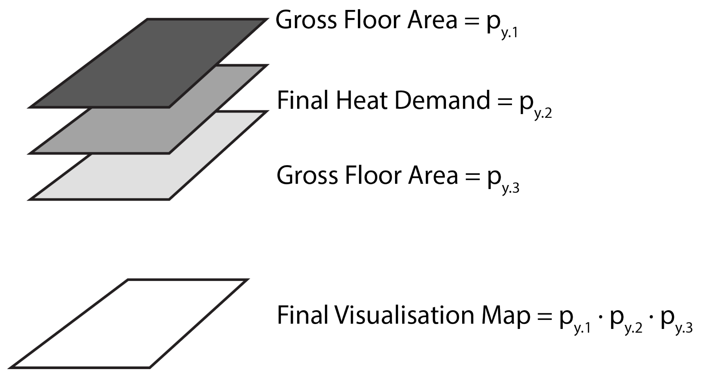
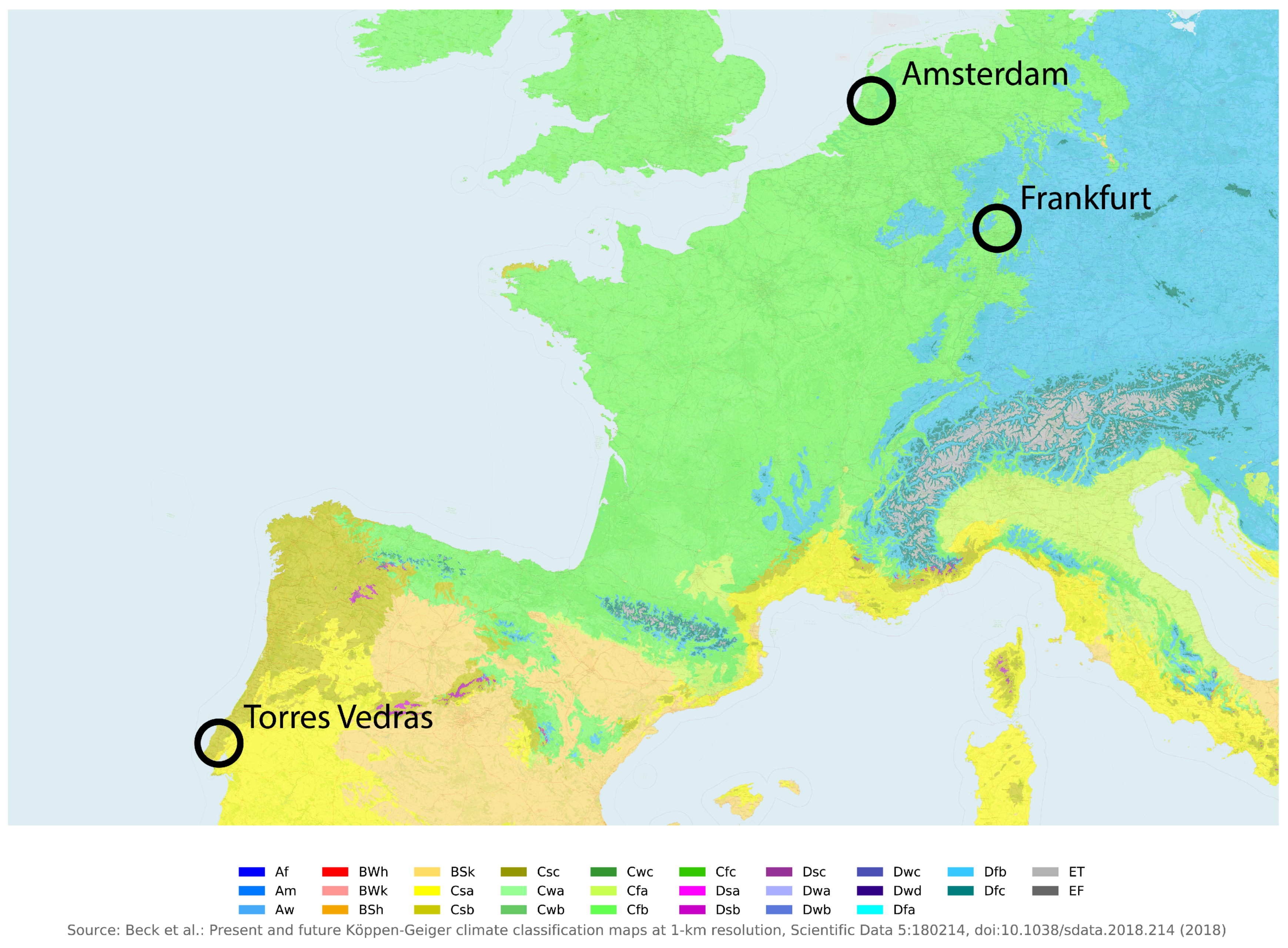
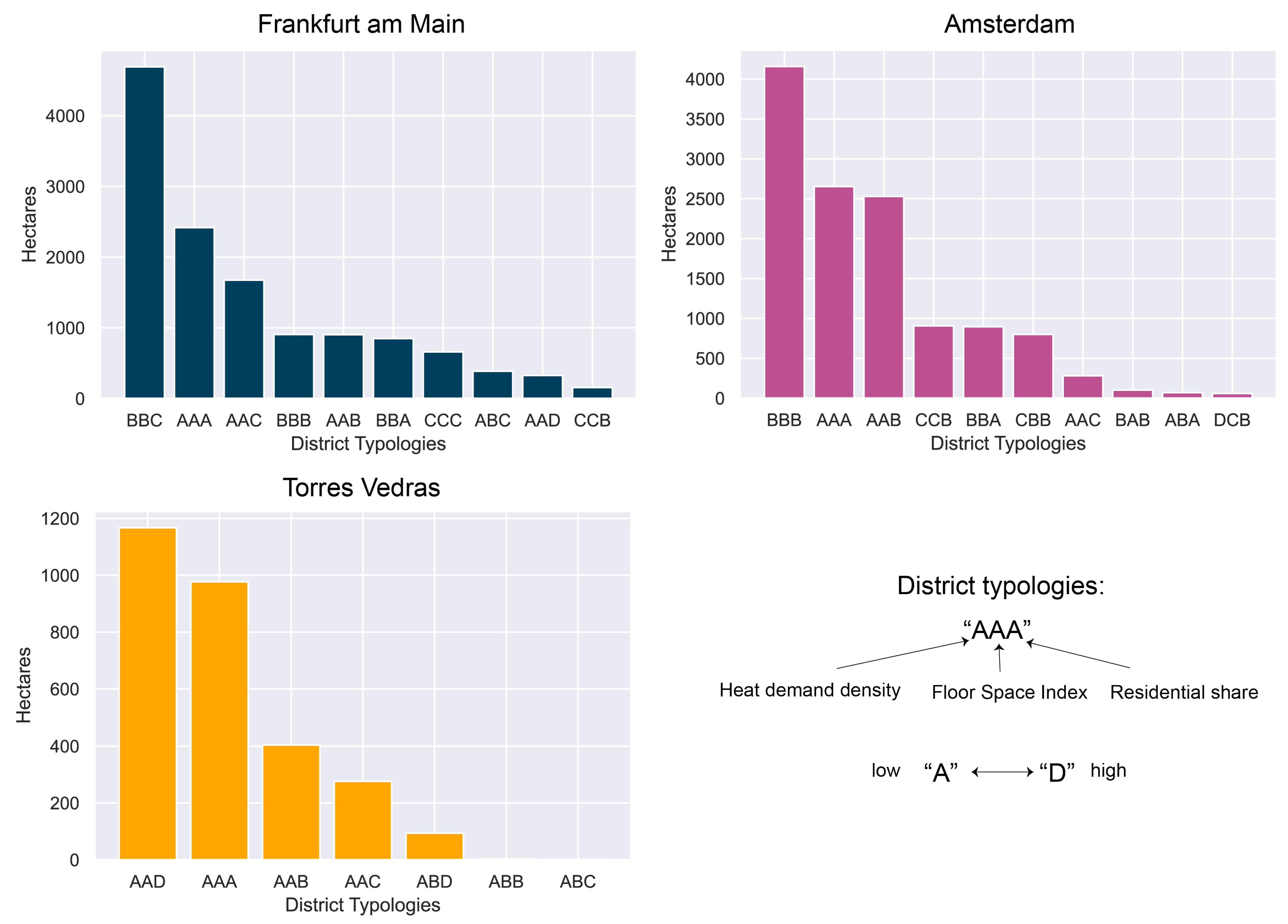
5. Visualisation of Results

This section shows the application of the approach presented in Section 3 to three European districts. Figure 6 shows a map of the different climate zones according to the Köppen–Geiger classification across Europe, which was used to filter out districts of interest located in the same climate zone. For further discussion, three partner cities of the "Smart-BEEjS" project for PEDs were selected [39]. Amsterdam and Frankfurt are located in the same climate zone of Cfb (temperate oceanic climate). In contrast, Torres Vedras in the south of Europe is characterised by the Csb climate zone (warm-summer Mediterranean climate). Thus, according to the first layer of diversification, districts in Amsterdam and Frankfurt could be used for comparison. The different climate in Torres Vedras might already have different implications for the energy infrastructures of potential districts; therefore, Torres Vedras could not be compared to the two other cities.
Figure 7 zooms into the three cities of Frankfurt, Amsterdam and Torres Vedras to visualise their district typologies in further detail. Areas that are presented in purple, red or even light orange have increasingly dense heat demands, higher floor space indices and larger shares of residential building usage. Conversely, green areas are less dense and indicate mixed-use or even low residential districts. As this map aimed to compare (but not rank) districts, the order of district combinations in the legend is of little importance. It is simply the result of the prime number approach described in Appendix B. The prime numbers were back-calculated to the respective alphabetical code. The colour code just provides an indication of the density. Additionally, not all of the 64 theoretically possible combinations appear in Europe.
Frankfurt and Amsterdam are similar in size and also show a comparable picture in terms of the district typologies that are present. Both cities show a highly dense centre that is shaded in red/violet, but the central area in Amsterdam is larger and denser. The dense, red-shaded areas are surrounded by blue and then green zones. Frankfurt appears to have multiple smaller settlements around the core city, while Amsterdam seems to be more connected. At the edges of the city and in the canal zones, Amsterdam is mainly shaded in light green. This most likely shows highly industrial areas and ports. Torres Vedras, on the other hand, is predominantly shaded in green and only peaks at light blues in the city centre. This, combined with the warmer climate zone, suggests advantages in terms of the required energy infrastructure for a PED as the heating demand is lower, the potential solar gains are higher, and the available space for local energy generation is larger.
These observations were supported by histograms of the district typologies of the cities. Figure 8 shows the size of each of the ten most common district typologies (in hectares) across the whole cities (Torres Vedras only has seven). The three most common typologies in Frankfurt and Amsterdam are very similar. Both show medium-low heat demands and floor space indices. Amsterdam, however, seems to be slightly less residential and has more highly dense areas within the ten most common categories, such as CCB. Torres Vedras, on the other hand, shows an entirely different picture. The city has a low heat demand thanks to its climate and also a very low floor space index in most areas. The town is very residential but has highly non-residential zones surrounding it, which are most likely industrial or commercial areas.
Torres Vedras is not located within the same climate zone as Frankfurt and Amsterdam (Figure 6) and, therefore, was filtered out by the climate layer as it could not be compared to the other two cities. As Amsterdam and Frankfurt are located within the same climate zone, two example districts were selected to compare according to their district typologies. A PED project called Atelier is located in the south of Buiksloterham in Amsterdam [40]. In Frankfurt, the Griesheim-Mitte district also has major renovation ambitions [41]. Figure 9 shows the distributions of the available district typologies in Frankfurt (Griesheim-Mitte) and Amsterdam (southern Buiksloterham). First of all, Griesheim-Mitte is significantly larger than southern Buiksloterham. Secondly, both districts have predominantly low to medium heating demands and F S I values. However, buildings in Griesheim-Mitte have higher levels of residential usage than those in southern Buiksloterham. Furthermore, southern Buiksloterham shows many areas with low heating demands and F S I values, with AAB, AAA and AAC being among the five most common areas within the district. On the contrary, Griesheim-Mitte has few areas with higher heating demands and F S I values, with CCC and CCB being in the top five categories. As southern Buiksloterham has, on average, lower heating demands and F S I values, there is more available space for energy generation, in the form of solar PV or solar thermal panels, in relation to the energy demand. Furthermore, the lower share of residential buildings could be beneficial for the self-supply of the district as commercial energy demands may be more aligned with sun hours and, thus, with renewable energy generation. The comparison indicated a relatively low similarity between the districts and, therefore, limited potential for knowledge transfer among the districts.
Figure 10 and Figure 11 show aerial views of Griesheim-Mitte and the considered part of Buiksloterham, respectively. The figures support our analysis of the district histograms well and, therefore, also act as validation for the created map. First of all, the size difference between the two districts is evident. Moreover, a large share of the BBC areas in Griesheim-Mitte is seen towards the mid-right of the district in Figure 10, which are predominantly made up of residential buildings. On the other hand, southern Buiksloterham has a small residential area in the lower-left corner with more prominent areas of non-residential buildings, according to the aerial view. Finally, the floor space index appears to be lower at first glance. These observations were consistent with the previously discussed histograms in Figure 9.

6. Conclusions

In light of the energy transition process that is partly facilitated by positive energy districts across Europe, methods that enable comparability of such district projects and thus encourage learning among them is becoming vital. One of the important aspects of creating PEDs is the physical energy infrastructure that is necessary for an existing district to transform into a PED. This article presented a method to facilitate district comparison regarding their energy infrastructure requirements. This work derived four indicators from the literature on energy system modelling: climate, heating demands, floor space index and the share of residential buildings. Furthermore, this study applied the developed methodology using QGIS and data that were openly available from the Hotmaps project, which led to a direct visualisation of each hectare of the cities and districts within Europe, thereby enabling an easy and direct comparison of the different areas. This clustering approach could facilitate the comparison of districts that are very similar according to the developed indicator values. The clustering methodology could also help districts to learn from the successes and challenges that arose in previous energy renovation projects that occurred in similar district categories. The example application using the districts of Griesheim-Mitte in Frankfurt and southern Buiksloterham in Amsterdam indicated the potential of this method for comparing districts.
Beyond this, the map also indicated which zones would be more challenging to convert into PEDs and could therefore work complementarily with the method of [9], which also shows which zones would be the most and least suitable for PEDs using a GIS-based approach. In our map, zones that are coloured in orange or red have high heat demands, high floor space indices and high shares of residential buildings. Those attributes increase the difficulty of achieving PED status as energy loads are less distributed and less space is available for energy generation in relation to the higher energy demands. On the contrary, green zones will likely be easier to convert into PEDs. This information could be vital in district-level renovation projects. It could allow for the differentiation of the areas within a district that require the most attention from a technical standpoint from the areas that could provide the energy generation surplus that is needed to achieve a positive balance overall. Based on the same information, would also be possible to evaluate whether a district needs renewable energy production outside of the district’s boundaries to offset its consumption. This analysis could estimate to what extent building stocks need to be improved or how much PV production would be required. Assuming that some energy production would need to be positioned outside of a district, this method could also suggest whether regional electrical infrastructures require further improvement. As of now, the aim of the visualisation map is only to compare districts and potentially transfer knowledge among similar projects. These further applications would require more PED (or PED-like) projects in existing areas and, subsequently, validation.
As stated in Section 1, there are currently only two PEDs operating in Europe, which limits the amount of information that is available regarding the implemented infrastructures. Furthermore, these two PEDs are newly built and are not renovation projects. As the number of implemented PEDs increases in the near future, the addition of more marked areas on the map will become possible. As the map shows data from 2015, it shows district typologies from before any renovations. These future additions would allow local policymakers and administrations to locate implemented PED projects that match their district typology and learn from those already existing projects. The two-layer visualisation map could also be used as an initial step for tracking existing PED projects over time and pinpointing them on the map as a working document. Readers should note that this categorisation comprises only four parameters. District renovations often require a holistic approach that also includes the social fabric of the area in question. Although a solution that was derived from another similar project may be technically feasible in a local context, it may be not socially accepted. This issue, combined with the estimated nature of the data that were used to develop the district typology map, should remind readers that this tool is intended for initial planning and policymaking based on findings from other projects. Thus, the map could be used as the first tool for PED planning to identify projects in similarly structured districts for knowledge transfer.
Further detailed research and calculations are necessary for specific districts as there may be other aspects that need to be considered, e.g., the availability of waste heat. Future research should focus on further verifying whether this method leads to two different districts within the same classification having similar infrastructures to achieve PED status. In addition, it is possible to create other typology and raster maps for different aims and visualisations. Other future work, still revolving around the necessary infrastructures, should focus on whether there is enough energy generation potential in relation to demand at a hectare level. It could be possible to compare the solar PV yearly potential raster to the yearly heat demand and obtain a rough estimate of the energy balance. Overall, this would be an initial step towards creating comparability in terms of buildings and energy infrastructures among European districts.
The limitations of our approach were closely related to the limitations of the Hotmaps data. The gross floor area was calculated using the average gross floor area per dwelling and the average persons per household, based on the available statistical data at the NUTS3 level (e.g., “Landkreise” in Germany). While this approach provided a reasonable estimation for residential building stocks at a hectare level, the non-residential gross floor area calculation was less robust [20]. The heat demand data were calculated at the NUTS0 level (country level) from the statistical data on energy consumption, as well as the national building stock characteristics. The grid cell-specific energy demand per floor area data were derived from the surface to volume ratios of buildings from the OpenStreetMap database, the shares per construction period and the heating and cooling degree days [20]. Each of these indicators were estimations in themselves and thus, were limited in their accuracy. Furthermore, the validation of the model was only based on aerial views of the studied districts. While this provided an initial indication of the model’s validity, further studies still need to prove this.

Author Contributions

Conceptualisation, A.B., L.C., A.A., L.K. and K.G.; methodology, A.B., L.C., A.A. and L.K.; validation, A.B., L.C. and A.A.; formal analysis, A.B., L.C. and A.A.; investigation, A.B., L.C. and A.A.; resources, A.B., L.C. and A.A.; data curation, A.B., L.C. and A.A.; writing—original draft preparation, A.B., L.C. and A.A.; writing—review and editing, A.B., L.C., A.A., L.K. and K.G.; visualisation, A.B., L.C. and A.A.; supervision, L.K. and K.G.; project administration, K.G.; funding acquisition, K.G. All authors have read and agreed to the published version of the manuscript.

Funding

This research received funding from the European Union’s Horizon 2020 research and innovation programme under the Marie Skłodowska-Curie Actions programme (grant number 812730).

Institutional Review Board Statement

Not applicable.

Informed Consent Statement

Not applicable.

Data Availability Statement

The data used in this study is taken from https://gitlab.com/hotmaps accessed on 17 June 2022 and https://doi.org/10.1038/sdata.2018.214. The derived map is publicly accessible under https://doi.org/10.5281/zenodo.6719747.

Conflicts of Interest

The authors declare no conflict of interest.

Abbreviations

The following abbreviations are used in this manuscript:
DCMDistrict Categorisation Matrix
DHDistrict Heating
EVElectric Vehicle
F S I Floor Space Index
HVACHeating, Ventilation and Air Conditioning
KPIKey Performance Indicator
PEDPositive Energy District
PVPhotovoltaic Panel

Appendix A

Table A1. A list of the reviewed models.
ModelAim/OutputRequirement/InputMethodTime ResolutionSpatial AspectSectors
Calliope [44,45,46]Energy portfolio and dispatch optimisationDemand profiles, technology to consider, available area, meteorological data and costsBottom-up; MILPUser definedUser definedElectricity, heating and mobility (limited)
City-BES [47]User defined, e.g., energy-, emissions- and cost-related KPIs for each retrofit scenarioThe footprint, type, height, year of construction and number of stories of the buildings, shading buildings, shared walls and weatherBottom-up; physics-based (based on EnergyPlus)Sub-hourlyCitiesElectricity and heating
City Energy Analyst [48]Building energy consumption patterns in neighbourhoods and districtsWeather data, urban GIS data building archetypes, distributions database (occupancy schedules; 16 types in this case) and measurements database (for non-standardised energy services in the area, e.g., stadia)Bottom-up (two methods of load calculation: analytical and statistical)HourlyNeighbourhoodsElectricity and heating
CitySim [49]Heating and cooling demands and urban planningBuilding characteristics and climate filesDynamic building energy simulation; reduced-order RC model1 min–1 hStreets to districtsElectricity and heating
DER-CAM [50]Energy portfolio and dispatch optimisationDemand profiles, technology to consider, available area, meteorological data and costsBottom-up; MILPUser defined (reference: days)Buildings to microgrids (districts)Electricity, heating and mobility (limited)
DIMOSIM [51]Raw outputs, i.e., states of each object (e.g., temperature) and energy fluxes (e.g., consumption per fuel) and KPIs generated from the raw outputs that related to thermal indoor comfort, energy, power and costsClimatic characteristics, building geometry, U-values and surface ratios of the different components within the envelope, HVAC system characteristics, occupancy rates, insulation types (e.g., indoor or outdoor) and inertia levelBottom-up; simulation; possible optimisationUser defined (range of minutes to hours)Small neighbourhoods to citiesElectricity and heating
EnergyPlan [52]Operation of energy systems and environmental and economic impactsInstalled capacity, available energy and energy demandsBottom-up; simulation (based on heuristic technique)HourlyCities to countriesElectricity and heating
EnergyPlus [53]Dynamic building simulations and HVACClimate data, U- and g-values, heating and cooling systems, temperature set-point (min; max), air change per hour, internal heat gain, external short-wave absorbance and long-wave emissivityBottom-up; physics-basedUser definedBuildingsElectricity and heating
ESP-r [54]Dynamic building simulations and HVACClimate data, U- and g-values, heating and cooling systems, temperature set-point (min; max), air change per hour, internal heat gain, external short-wave absorbance and long-wave emissivityBottom-up; physics-basedUser definedBuildings to districtsElectricity and heating
Homer [55]Energy portfolio and dispatch optimisationDemand profiles, technology to consider, available area, meteorological data and costsBottom-upUser definedMicrogrids (districts)Electricity, heating and mobility (limited)
oemof [56]Multiple Python libraries for optimisation and modelling of energy systemsDemand profiles, technology to consider, available area, meteorological data and costsBottom-upUser defined (reference: days)Buildings to microgrids (districts)Electricity, heating and mobility (limited)
Smart-E [57]Energy demand simulation, implementation of demand–response strategies in citiesWeather data, household composition, envelope characteristics, heating energy demands, location, time of use (schedule) and probabilities (household equipment, set points, etc.)Bottom-up; simulationDailyCities to larger territoriesElectricity and heating
TRNSYS [58]Thermal and electrical energy systems, dynamic systems, traffic flow and biological processesUser defined components and library componentsSimulation; linear and nonlinear programming0.01 s–1 hBuildings to districtsElectricity, heating and mobility
urbs [59]Energy portfolio and dispatch optimisationDemand profiles, technology to consider, available area, renewable energy supplies as time series and costsBottom-upUser definedUser definedElectricity, heating and mobility (limited)
UMI [60]Walkability, environmental performance and daylight potentialParks, streets, shadings, boundaries, ground and the geometry, occupancy and fenestration of buildingsSimulation (based on EnergyPlus, rhinoceros and Daysim)Streets to districtsElectricity, heating and mobility

Appendix B

This section explains how we developed the map that categorises the districts and areas in Europe. The reasons for the selection of each parameter and their related thresholds are not subjected to further analysis here but rather the process itself for replication. The analysis that was conducted in Section 3 led to the selection of the relevant raster files from the Hotmaps repository. These raster files were:
  • Total gross floor area;
  • Residential gross floor area;
  • Final heat demand density.
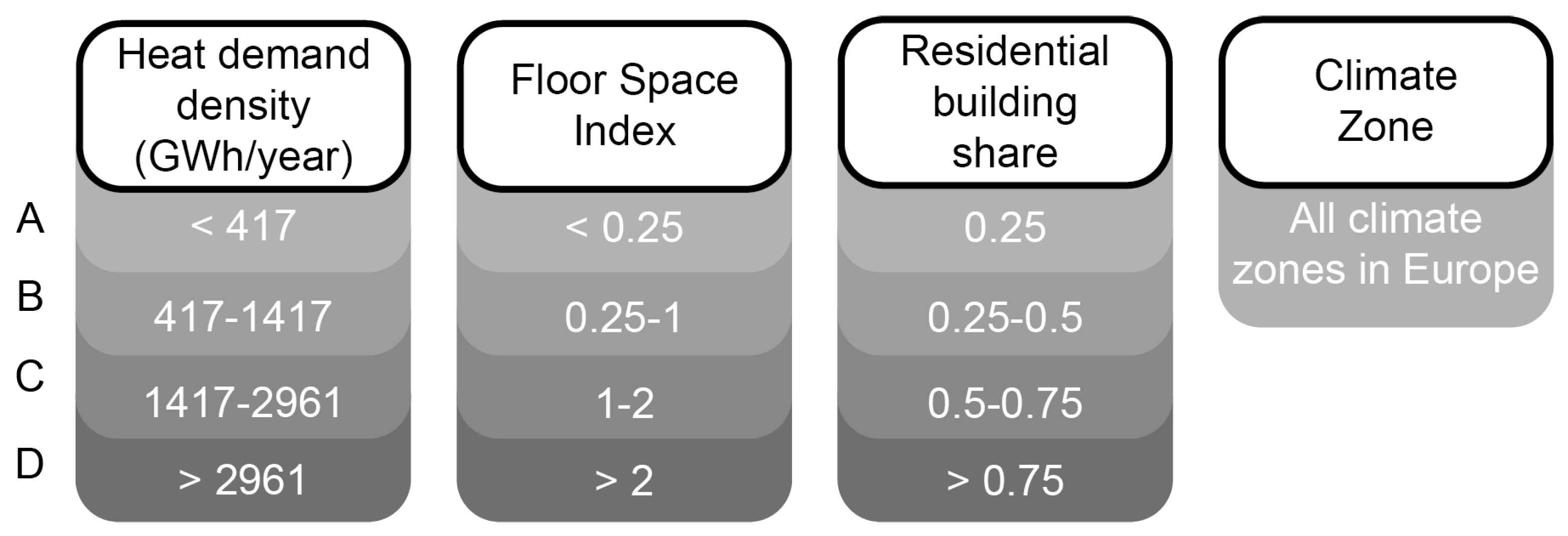
The first two rasters were relevant for producing the floor space index and the residential gross floor area percentage. To generate the latter, we utilised the raster calculator function in QGIS. We divided the residential gross floor area by the total gross floor area. Using a similar process, the total gross floor area was converted into an approximation of the F S I by simply dividing the raster by 10,000, as each pixel equalled one hectare and the pixel’s value was expressed in square meters. Section 3 already explained the reasons behind the selection of each threshold; hence, it is not part of this section. This section explains how the rasters were changed to show the thresholds rather than the values. Again, the raster calculator included in QGIS was the tool that was used to generate the typologies of these rasters. Four bands were generated by setting the following conditions on each raster file:
( ( R x > 0 ) A N D ( R x t 1 ) ) p 1 . x + ( ( R x > t 1 ) A N D ( R x t 2 ) ) p 2 . x + ( ( R x > t 2 ) A N D ( R x t 3 ) ) p 3 . x + ( R x > t 3 ) p 4 . x
where R a s t e r x is the raster subject to be transformed, t1 to t3 are the set thresholds and p 1 . x to p 4 . x indicate the prime numbers that were applied to the first to fourth bands of the x t h layer. Each threshold was defined by a prime number rather than a letter as QGIS does not support strings as a data type. The use of prime numbers allowed for the creation of the final visualisation map. The final visualisation map raster condensed the information from each pixel in the three rasters (i.e., total gross floor area, share of residential gross floor area and final heat demand density) into one raster, as shown in Figure A1. QGIS does not allow the multiplication or addition characters; hence, we used prime numbers to track the original values.
Figure A1. The process for blending the three original layers into the visualisation map. The subscript y indicates the band to which pixel belongs.
Energies 15 04720 g0a1
The prime numbers allowed us to retain the information from all of the layers that made up the map. The product of three prime numbers could only be obtained by multiplying those exact prime numbers. It is important to note that each threshold had a different prime number related to it, as indicated in Table A2.
Table A2. The code to transform letter indicators into prime numbers and vice versa.
ThresholdsLetter IndicatorPrime Number Indicator
Final Heat Demand Density417A2
417–1417B3
1417–2961C5
2961D7
Total Gross Floor Area0.25A9
0.25–1B11
1–2C13
2D17
Percentage of Residential GFA0.25A23
0.25–0.5B27
0.5–0.75C29
0.75D31
Let us consider an example in which a pixel on the map (i.e., one hectare) has a final heat demand that is indicated by A, a total gross floor area of B and a percentage of residential GFA of C. The resulting pixel on the visualisation map would have the value of the product of their prime number indicators (in this case, 638). Because this number can only be derived from the multiplication of these three prime numbers, each pixel can be unequivocally identified and categorised.

References

  1. United Nations Human Settlements Programme. Unpacking the Value of Sustainable Urbanization; World Cities Report 2020; UN: Nairobi, Kenya, 2020; pp. 43–74. [Google Scholar] [CrossRef]
  2. JPI Urban Europe. White Paper on PED Reference Framework for Positive Energy Districts and Neighbourhoods. 2020. Available online: https://jpi-urbaneurope.eu/wp-content/uploads/2020/04/White-Paper-PED-Framework-Definition-2020323-final.pdf (accessed on 21 June 2022).
  3. MAKING CITY. Making City—Energy Efficient Pathway for the City Transformation. Available online: https://makingcity.eu/ (accessed on 2 March 2022).
  4. +CityxChange. Available online: https://cityxchange.eu/ (accessed on 2 March 2022).
  5. IEA EBC. Annex 83-Positive Energy Districts. Available online: https://annex83.iea-ebc.org/ (accessed on 2 March 2022).
  6. POCITYF. Leading the Smart Evolution of Historical Cities. Available online: https://pocityf.eu/ (accessed on 2 March 2022).
  7. Bruck, A.; Díaz Ruano, S.; Auer, H. A Critical Perspective on Positive Energy Districts in Climatically Favoured Regions: An Open-Source Modelling Approach Disclosing Implications and Possibilities. Energies 2021, 14, 4864. [Google Scholar] [CrossRef]
  8. Bossi, S.; Gollner, C.; Theierling, S. Towards 100 positive energy districts in Europe: Preliminary data analysis of 61 European cases. Energies 2020, 13, 6083. [Google Scholar] [CrossRef]
  9. Alpagut, B.; Lopez Romo, A.; Hernández, P.; Tabanoğlu, O.; Hermoso Martinez, N. A GIS-Based Multicriteria Assessment for Identification of Positive Energy Districts Boundary in Cities. Energies 2021, 14, 7517. [Google Scholar] [CrossRef]
  10. JPI Urban Europe. Europe towards Positive Energy Districts; PED Booklet 2020; 180p, Available online: https://jpi-urbaneurope.eu/wp-content/uploads/2020/06/PED-Booklet-Update-Feb-2020_2.pdf (accessed on 21 June 2022).
  11. Zwickl-Bernhard, S.; Auer, H. Open-source modeling of a low-carbon urban neighborhood with high shares of local renewable generation. Appl. Energy 2021, 282, 116166. [Google Scholar] [CrossRef]
  12. Fulmer, J.E. What is the World Infrastructure? PEI Infrastruct. Investor 2009, 1, 30–32. [Google Scholar]
  13. Brozovsky, J.; Gustavsen, A.; Gaitani, N. Zero emission neighbourhoods and positive energy districts—A state-of-the-art review. Sustain. Cities Soc. 2021, 72, 103013. [Google Scholar] [CrossRef]
  14. Chang, M.; Thellufsen, J.Z.; Zakeri, B.; Pickering, B.; Pfenninger, S.; Lund, H.; Østergaard, P.A. Trends in tools and approaches for modelling the energy transition. Appl. Energy 2021, 290, 116731. [Google Scholar] [CrossRef]
  15. Siedentop, S.; Schiller, G.; Koziol, M.; Walther, J.; Gutsche, J.M. Siedlungsentwicklung und Infrastrukturfolgekosten—Bilanzierung und Strategieentwicklung; Technical Report 3; Bundesamt für Bauwesen und Raumordnung: Bonn, Germany, 2006. [Google Scholar]
  16. Nzengue, Y.; du Boishamon, A.; Laffont-Eloire, K.; Partenay, V.; Abdelouadoud, Y.; Zambelli, P.; D’Alonzo, V.; Vaccaro, R. Planning city refurbishment: An exploratory study at district scale how to move towards positive energy districts—Approach of the SINFONIA project. In Proceedings of the 2017 International Conference on Engineering, Technology and Innovation (ICE/ITMC), Madeira, Portugal, 27–29 June 2017; pp. 1394–1400. [Google Scholar] [CrossRef]
  17. Hachem-Vermette, C.; Singh, K. Optimization of energy resources in various building cluster archetypes. Renew. Sustain. Energy Rev. 2022, 157, 112050. [Google Scholar] [CrossRef]
  18. Hachem-Vermette, C.; Singh, K. Energy Systems and Energy Sharing in Traditional and Sustainable Archetypes of Urban Developments. Sustainability 2022, 14, 1356. [Google Scholar] [CrossRef]
  19. Pezzutto, S.; Croce, S.; Zambotti, S.; Kranzl, L.; Novelli, A.; Zambelli, P. Assessment of the space heating and domestic hot water market in Europe—Open data and results. Energies 2019, 12, 1760. [Google Scholar] [CrossRef] [Green Version]
  20. Hotmaps Project. Library-Hotmaps Project. Available online: https://www.hotmaps-project.eu/library/ (accessed on 21 June 2022).
  21. Müller, A.; Hummel, M.; Kranzl, L.; Fallahnejad, M.; Büchele, R. Open Source Data for Gross Floor Area and Heat Demand Density on the Hectare Level for EU 28. Energies 2019, 12, 4789. [Google Scholar] [CrossRef] [Green Version]
  22. Markovic, D.; Cvetkovic, D.; Masic, B. Survey of software tools for energy efficiency in a community. Renew. Sustain. Energy Rev. 2011, 15, 4897–4903. [Google Scholar] [CrossRef]
  23. Keirstead, J.; Jennings, M.; Sivakumar, A. A review of urban energy system models: Approaches, challenges and opportunities. Renew. Sustain. Energy Rev. 2012, 16, 3847–3866. [Google Scholar] [CrossRef] [Green Version]
  24. Allegrini, J.; Orehounig, K.; Mavromatidis, G.; Ruesch, F.; Dorer, V.; Evins, R. A review of modelling approaches and tools for the simulation of district-scale energy systems. Renew. Sustain. Energy Rev. 2015, 52, 1391–1404. [Google Scholar] [CrossRef]
  25. Huang, Z.; Yu, H.; Peng, Z.; Zhao, M. Methods and tools for community energy planning: A review. Renew. Sustain. Energy Rev. 2015, 42, 1335–1348. [Google Scholar] [CrossRef]
  26. Ferrari, S.; Zagarella, F.; Caputo, P.; Bonomolo, M. Assessment of tools for urban energy planning. Energy 2019, 176, 544–551. [Google Scholar] [CrossRef]
  27. Abbasabadi, N.; Mehdi Ashayeri, J.K. Urban energy use modeling methods and tools: A review and an outlook. Build. Environ. 2019, 161, 106270. [Google Scholar] [CrossRef]
  28. Klemm, C.; Vennemann, P. Modeling and optimization of multi-energy systems in mixed-use districts: A review of existing methods and approaches. Renew. Sustain. Energy Rev. 2021, 135, 110206. [Google Scholar] [CrossRef]
  29. Yazdanie, M.; Orehounig, K. Advancing urban energy system planning and modeling approaches: Gaps and solutions in perspective. Renew. Sustain. Energy Rev. 2021, 137, 110607. [Google Scholar] [CrossRef]
  30. Bouw, K.; Noorman, K.J.; Wiekens, C.J.; Faaij, A. Local energy planning in the built environment: An analysis of model characteristics. Renew. Sustain. Energy Rev. 2021, 144, 111030. [Google Scholar] [CrossRef]
  31. Kottek, M.; Grieser, J.; Beck, C.; Rudolf, B.; Rubel, F. World Map of the Köppen-Geiger climate classification updated. Meteorol. Z. 2006, 15, 259–263. [Google Scholar] [CrossRef]
  32. Beck, H.E.; Zimmermann, N.E.; McVicar, T.R.; Vergopolan, N.; Berg, A.; Wood, E.F. Present and future Köppen-Geiger climate classification maps at 1-km resolution. Sci. Data 2018, 5, 1–12. [Google Scholar] [CrossRef] [Green Version]
  33. Ascencio-Vásquez, J.; Brecl, K.; Topič, M. Methodology of Köppen-Geiger-Photovoltaic climate classification and implications to worldwide mapping of PV system performance. Solar Energy 2019, 191, 672–685. [Google Scholar] [CrossRef]
  34. PVSITES Consortium. D2.2 European Climate Zones and Bio-Climatic Design Requirements. Technical Report. 2016. Available online: https://ec.europa.eu/research/participants/documents/downloadPublic?documentIds=080166e5ac7b5027&appId=PPGMS (accessed on 21 June 2022).
  35. Leibold, J.; Schneider, S.; Tabakovic, M.; Zelger, T.; Bell, D.; Schöfmann, P.; Bartlmä, N. ‘Zukunftsquartier’—On the Path to Plus Energy Neighbourhoods in Vienna. In Sustainability in Energy and Buildings; Springer: Singapore, 2020; pp. 199–209. [Google Scholar] [CrossRef]
  36. Caves, R.W. Encyclopedia of the City; Routledge: Abingdon, UK, 2005. [Google Scholar]
  37. Hachem-Vermette, C.; Singh, K. Optimization of the mixture of building types in a neighborhood and their energy and environmental performance. Energy Build. 2019, 204, 109499. [Google Scholar] [CrossRef]
  38. Yuan, J.; Zhang, G.; Yu, S.S.; Chen, Z.; Li, Z.; Zhang, Y. A multi-timescale smart grid energy management system based on adaptive dynamic programming and Multi-NN Fusion prediction method. Knowl. Based Syst. 2022, 241, 108284. [Google Scholar] [CrossRef]
  39. Smart-BEEjS. Innovative Training Network—Smart Value Generation by Building Efficiency and Energy Justice for Sustainable Living. Available online: https://smart-beejs.eu/ (accessed on 21 June 2022).
  40. ATELIER. ATELIER-Positive Energy Districts. Available online: https://smartcity-atelier.eu/ (accessed on 21 June 2022).
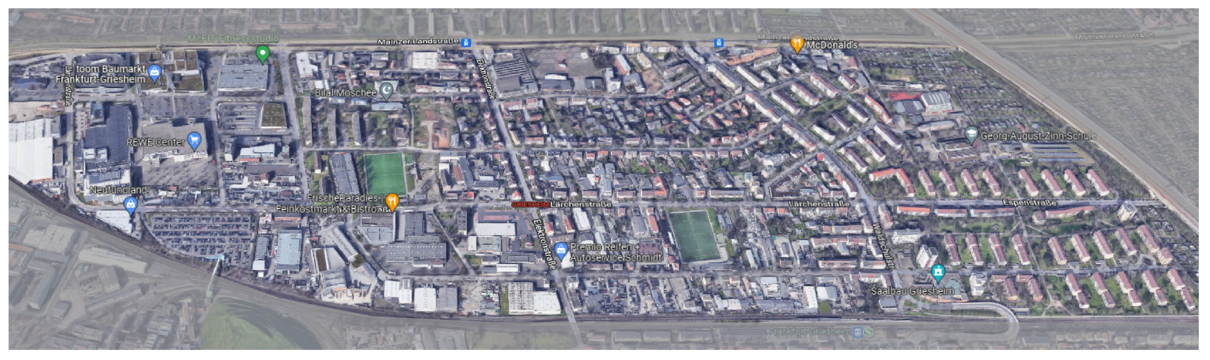
  41. Stadt Frankfurt am Main. Frankfurt a.M. Griesheim-Mitte—Integriertes Städtebauliches Entwicklungskonzept; Technical Report; Stadtplanungsamt Frankfurt am Main: Frankfurt, Germany, 2019. [Google Scholar]
  42. Google Maps. Griesheim-Mitte—Google Maps. Available online: https://www.google.com/maps/place/Griesheim,+Frankfurt,+Germany/@50.0983916,8.5985339,15.3z/data=!4m5!3m4!1s0x47bd0a2fd4be4e49:0x522435029b39a00!8m2!3d50.0965406!4d8.5987565 (accessed on 21 June 2022).
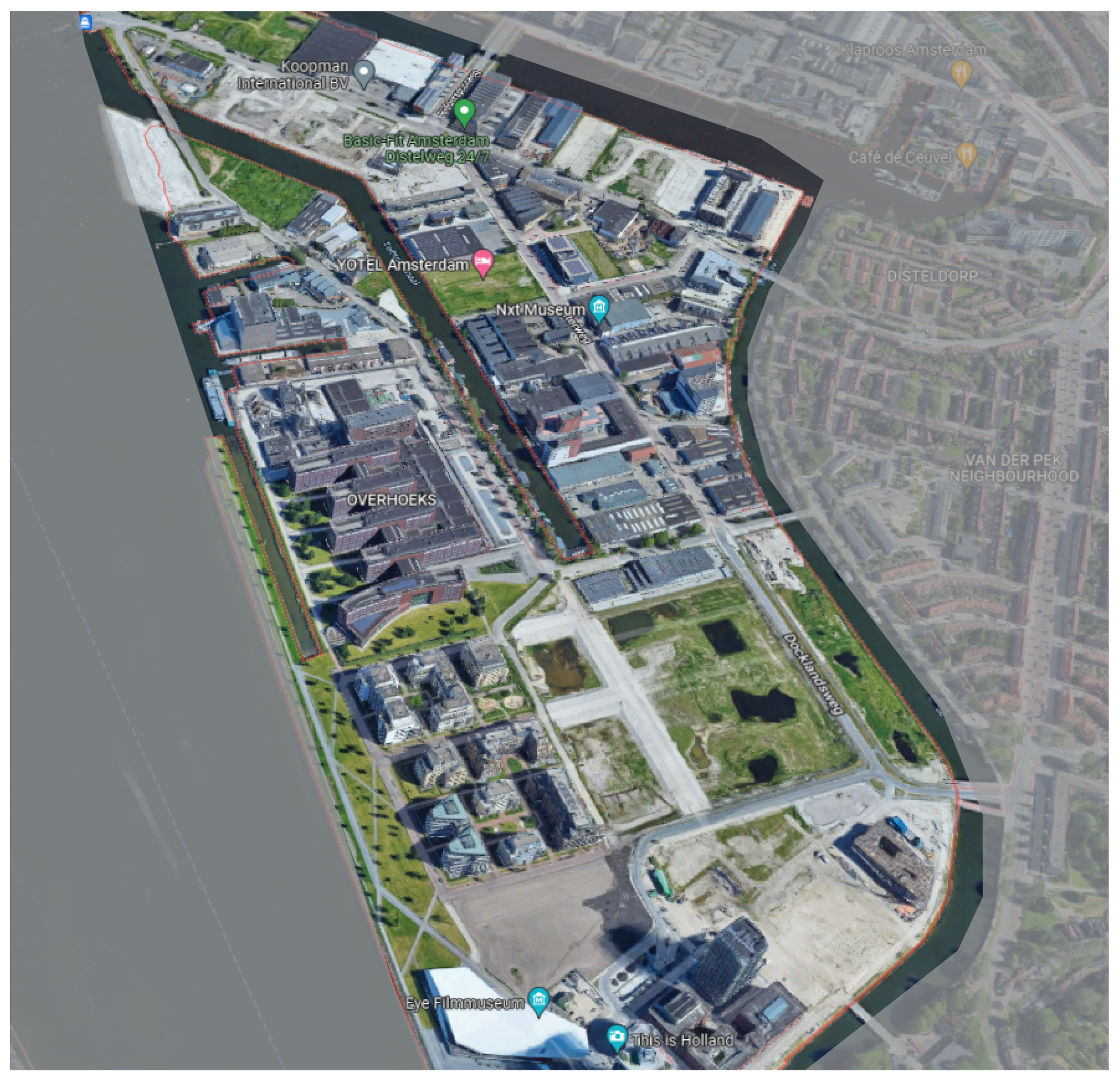
  43. Google Maps. Buiksloterham-South—Google Maps. Available online: https://www.google.com/maps/place/Buiksloterham,+Amsterdam,+Netherlands/@52.3901559,4.8951995,15.56z/data=!4m5!3m4!1s0x47c6083a59bcc9b5:0x5b0aa59876a0ead1!8m2!3d52.401543!4d4.8907417 (accessed on 21 June 2022).
  44. Pfenninger, S.; Pickering, B. Calliope: A multi-scale energy systems modelling framework. J. Open Source Softw. 2018, 3, 825. [Google Scholar] [CrossRef] [Green Version]
  45. Calliope: A multi-Scale Energy Systems Modelling Framework—Calliope 0.6.7 Documentation. Available online: https://calliope.readthedocs.io/en/stable/ (accessed on 15 December 2021).
  46. Luz, G.P.; E Silva, R.A. Modeling Energy Communities with Collective Photovoltaic Self-Consumption: Synergies between a Small City and a Winery in Portugal. Energies 2021, 14, 323. [Google Scholar] [CrossRef]
  47. Chen, Y.; Hong, T.; Piette, M.A. Automatic generation and simulation of urban building energy models based on city datasets for city-scale building retrofit analysis. Appl. Energy 2017, 205, 323–335. [Google Scholar] [CrossRef] [Green Version]
  48. Fonseca, J.A.; Nguyen, T.A.; Schlueter, A.; Marechal, F. City Energy Analyst (CEA): Integrated framework for analysis and optimization of building energy systems in neighborhoods and city districts. Energy Build. 2016, 113, 202–226. [Google Scholar] [CrossRef]
  49. Walter, E.; Kämpf, J.H. A Verification of CitySim Results Using the BESTEST and Monitored Consumption Values; Bozen-Bolzano University Press: Bozen-Bolzano, Italy, 2015; pp. 215–222. [Google Scholar]
  50. DER-CAM|Grid Integration Group. Available online: https://gridintegration.lbl.gov/der-cam (accessed on 15 December 2021).
  51. Garreau, E.; Abdelouadoud, Y.; Herrera, E.; Keilholz, W.; Kyriakodis, G.E.; Partenay, V.; Riederer, P. District MOdeller and SIMulator (DIMOSIM)—A dynamic simulation platform based on a bottom-up approach for district and territory energetic assessment. Energy Build. 2021, 251, 111354. [Google Scholar] [CrossRef]
  52. Lund, H.; Thellufsen, J.Z.; Østergaard, P.A.; Sorknæs, P.; Skov, I.R.; Mathiesen, B.V. EnergyPLAN—Advanced analysis of smart energy systems. Smart Energy 2021, 1, 100007. [Google Scholar] [CrossRef]
  53. Crawley, D.B.; Pedersen, C.O.; Lawrie, L.K.; Winkelmann, F.C. EnergyPlus: Energy Simulation Program. ASHRAE J. 2000, 42, 49–56. [Google Scholar]
  54. Energy Systems Research Unit, University of Strathclyde. A Tour of ESP-r. Available online: https://www.esru.strath.ac.uk//Courseware/ESP-r/tour/ (accessed on 21 June 2022).
  55. HOMER—Hybrid Renewable and Distributed Generation System Design Software. Available online: https://www.homerenergy.com/ (accessed on 15 December 2021).
  56. Hilpert, S.; Kaldemeyer, C.; Krien, U.; Günther, S.; Wingenbach, C.; Plessmann, G. The Open Energy Modelling Framework (oemof)—A new approach to facilitate open science in energy system modelling. Energy Strategy Rev. 2018, 22, 16–25. [Google Scholar] [CrossRef] [Green Version]
  57. Berthou, T.; Duplessis, B.; Rivière, P.; Stabat, P.; Casetta, D.; Marchio, D. Smart-E: A tool for energy demand simulation and optimization at the city scale. In Proceedings of the 14th Conference of International Building Performance Simulation Association, Hyderabad, India, 7–9 December 2015; pp. 1782–1789. [Google Scholar]
  58. Klein, S.A. TRNSYS 18: A Transient System Simulation Program; Solar Energy Laboratory, University of Wisconsin: Madison, WI, USA, 2018. [Google Scholar]
  59. Dorfner, J. Urbs: A Linear Optimisation Model for Distributed Energy Systems 2022. Available online: https://urbs.readthedocs.io/en/latest/ (accessed on 21 June 2022).
  60. Reinhart, C.F.; Cerezo Davila, C. Urban building energy modeling—A review of a nascent field. Build. Environ. 2016, 97, 196–202. [Google Scholar] [CrossRef] [Green Version]
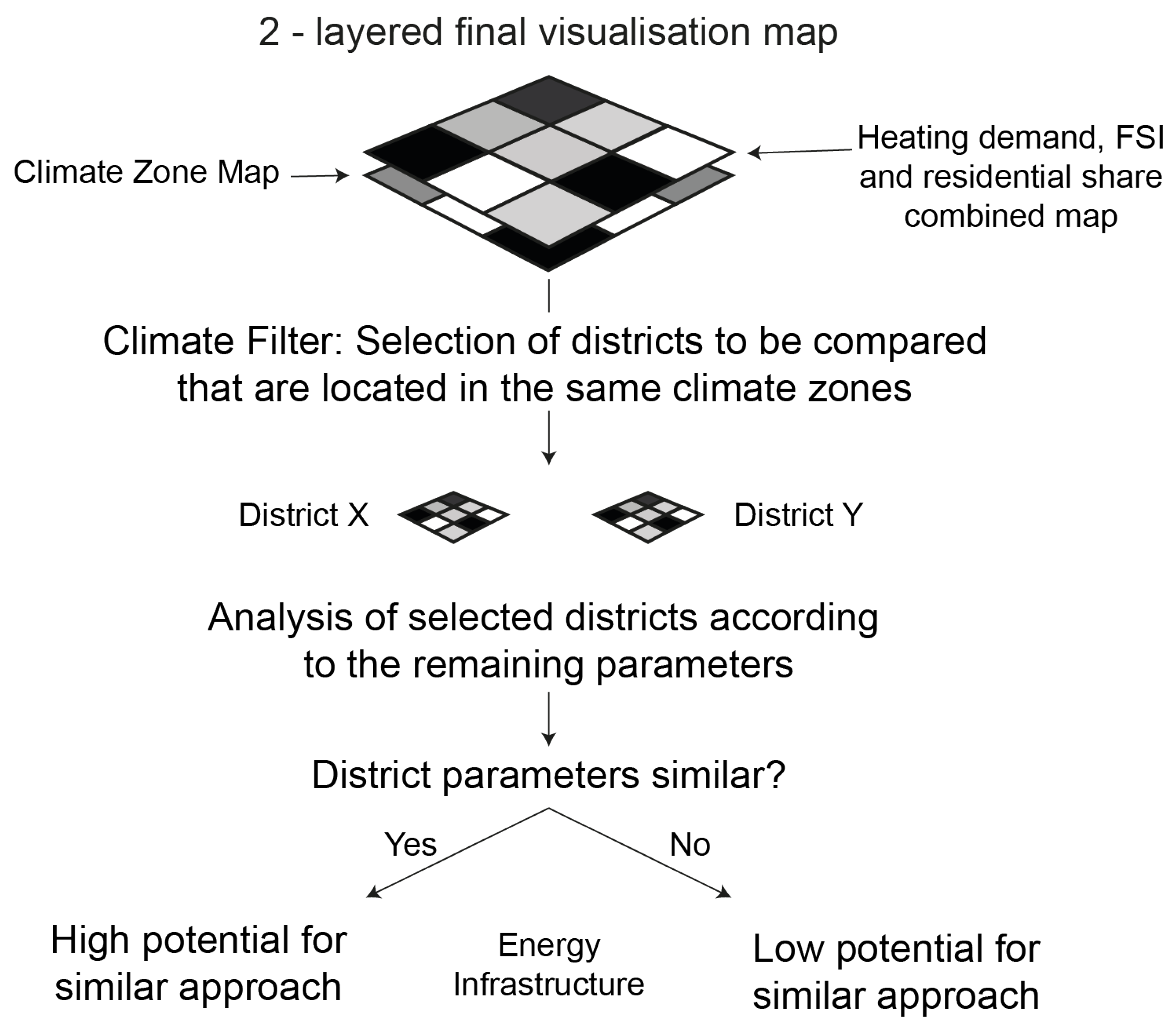
Figure 1. The key concepts/elements of positive energy districts (adapted from [2]).
Energies 15 04720 g001
Figure 2. Our methodological approach to classifying districts from an energy modelling point of view.
Energies 15 04720 g002
Figure 3. The district categorisation matrix.
Energies 15 04720 g003
Figure 4. Our methodological approach for the visualisation of the selected parameter combinations on a map.
Energies 15 04720 g004
Figure 5. The application process of the final district visualisation map.
Energies 15 04720 g005
Figure 6. A map of Central Europe, with climate zones according to the Köppen–Geiger classification [32]. Amsterdam, Frankfurt and Torres Vedras are marked on the map.
Energies 15 04720 g006
Figure 7. The visualisation of the district typologies in Frankfurt am Main (a), Amsterdam (b) and Torres Vedras (c): FHDD, final heat demand density; F S I , floor space index; %Rdt., share of residential buildings.
Energies 15 04720 g007
Figure 8. A comparison of the frequency of the district categories in Frankfurt am Main, Amsterdam and Torres Vedras.
Energies 15 04720 g008
Figure 9. A comparison of the frequency of the district categories in Frankfurt—Griesheim-Mitte am Main and Amsterdam—Buiksloterham-South.
Energies 15 04720 g009
Figure 10. An aerial view of Griesheim-Mitte [42].
Energies 15 04720 g010
Figure 11. An aerial view of southern Buiksloterham [43].
Energies 15 04720 g011
Table 1. The synthesis of parameters for the district categorisation.
Matching Data Requirements Representative Parameters
Meteorological data, renewable energy supplies, weather data and climatic characteristicsClimate Zone
Demand profiles, building envelopes, U-values, insulation and household equipmentHeating Demand
Available area, building type, building height, building archetype and building geometryFloor Space Index
Occupancy behaviour, time of use, net energy demands and PV productionShare of Residential Buildings
Publisher’s Note: MDPI stays neutral with regard to jurisdictional claims in published maps and institutional affiliations.

