Abstract
Explainable Artificial Intelligence (XAI) methods demonstrate internal representation of data hidden within neural network trained weights. That information, presented in a form readable to humans, could be remarkably useful during model development and validation. Among others, gradient-based methods such as Grad-CAM are broadly used in an image processing domain. On the other hand, the autonomous vehicle sensor suite consists of auxiliary devices such as radars and LiDARs, for which existing XAI methods do not apply directly. In this article, we present our adaptation approach to utilize Grad-CAM visualization for LiDAR pointcloud specific object detection architectures used in automotive perception systems. We try to solve data and network architecture compatibility problems and answer the question whether Grad-CAM methods could be used with LiDAR sensor data efficiently. We showcase successful results of our method and all the benefits that come with a Grad-CAM XAI application to a LiDAR sensor in an autonomous driving domain.
1. Introduction
Recent advances in the machine learning domain have resulted in more and more state-of-the-art solutions in a camera image processing, and many other applications are based on neural network architectures. These solutions, however, are often treated as so called methods [1], meaning that, given a particular input, they output some predictions, but an internal data processing is more or less unknown. This approach yields many doubts, especially in the domain of autonomous driving, where the variety of processed scenes is enormous and it is unclear whether a new situation, not tested at a development stage, will be correctly classified. Moreover, this is directly connected to safety issues and regulations, as decisions made based on such results could affect human lives.
To resolve this matter, a new branch of research, called explainable artificial intelligence (XAI), is being developed. The purpose of XAI is to explain the inner workings of processing the data by a neural network in a way that the decision-making process can be understood by humans [2,3]. Using the XAI methods, a neural network-based solution could be more reliably evaluated in the context of safety regulations. Even if such evaluation is not required for a particular application, the XAI methods could also help researchers better understand machine learning models and, based on that knowledge, introduce improvements to overall performance.
Explainable artificial intelligence is also considered in autonomous vehicle (AV) systems development [4]. Among other sub-systems, such as a localization or a path planning, an AV perception is crucial for the decision making and all other components relay on it. Perception systems use neural networks to process sensor data and create a model of the environment. Currently, the most common sensor suite used in AV perception systems consists of many cross-domain devices such as cameras, radars, and LiDARs. The XAI methods related to camera image processing and object detection networks are well developed as they were adopted from other vision tasks. Gradient-based methods [5,6,7] prove to be especially useful as they can show the importance of each input pixel in a final prediction output in the form of a heatmap. Unlike the vision images, however, sensor data from radars and LiDARs, which come in the form of a pointcloud, lack such XAI methods.
Addressing the problem of lacking XAI methods, our main contributions in this paper are as follows:
- Adaptation of an XAI Gradient-based Class Activation Maps (Grad-CAM) method used in camera image processing to a LiDAR object detection domain in order to visualize how an input pointcloud data affects the results of a neural network.
- In-depth analysis of key components and changes that need to be performed in order to apply the Grad-CAM method to pointcloud-specific neural network architecture based on voxel-wise pointcloud processing and single shot detector with a multi-class and multi-feature grid output.
- Usage of a Sparsity Invariant convolutional layer, from LiDAR depth-completion domain, which addresses a sparse nature of voxel-wise processed pointcloud data, for both object detection performance and quality of generated Grad-CAM heatmaps.
- Experiments conducted on LiDAR pointcloud data from popular autonomous driving KITTI [8] dataset and presentation of obtained results for proposed methods with comparison of pros and cons between them.
This paper is structured as follows. In Section 2, we go over related work regarding gradient-based methods used for vision tasks and explain neural network architectures for LiDAR pointcloud object detection. In Section 3, we present our approach to adapting those XAI methods to a LiDAR data format and network structure. Section 4 contains a description of our conducted experiments and results, as well as problems encountered and proposed solutions. Finally, we draw our conclusions in Section 5.
2. Related Work
2.1. Gradient-Based Methods
Explainable artificial intelligence methods are already widely applied to computer vision problems. Analysis of an input image processing could be easily shown in graphical form, as this is the same visual domain as the neural network internal representation. In [5], the authors proposed a method of visualizing Class Activation Maps (CAMs). To generate such maps, two components are required: activations from last convolutional layer and weights for each activation (Figure 1). The weighted sum of those activations form a visual heatmap called CAM.
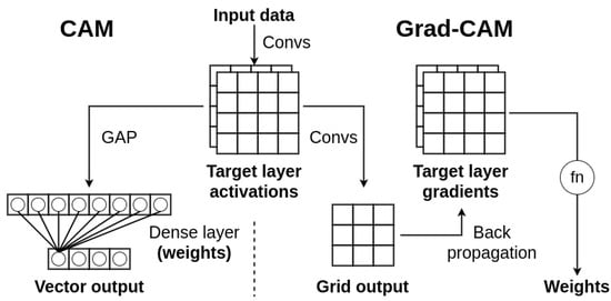
Figure 1.
Algorithm scheme comparison between CAM and Grad-CAM methods. Target activations are the same for both methods. The difference is observed in activation weights; in CAM, we derive them from dense layer weights, whereas in Grad-CAM we use backpropagation to obtain gradients of target layers and calculate weights based on them.
The activations are calculated during a forward pass of the neural network. To obtain the weights, these authors proposed a method consisting of a Global Average Pooling (GAP) layer followed by a fully-connected (FC) output layer. The GAP creates vector of importance values per activation, and the FC layer yields classification for each class based on this vector. Then, extracting FC layer weights for each class provides weights of each activation in a final Class Activation Map.
A significant drawback of that method is the architectural requirement of a final, fully-connected layer which does not belong in fully-convolutional models. This, however, is not an issue with Grad-CAM [6], which can be applied to both fully-connected and convolutional output layers. In addition, calculating CAMs with Grad-CAM is not constrained to the last convolutional layer, but rather it could be achieved for any given intermediate convolutional layer in the network architecture. The main principle of generating CAMs remains the same, but Grad-CAM relies on a backpropagation method to calculate gradients of a classification score with respect to a chosen convolutional layer activation. The weight of each activation is then determined based on those gradients values. In our original paper, the weights are calculated by taking a mean of gradients values along tensor dimensions corresponding to input image’s width and height. A more complex weight calculation is shown in Grad-CAM++ [7], where the authors introduced pixel-wise significance of the gradients values based on its spatial position in the feature map during calculation of the mean.
Gradient-based methods to generate Class Activation Maps prove to be very flexible in terms of usage for different network architectures and layers as well as methods of calculating activations weights based on gradient values. Those features allow us to adapt them to a completely new LiDAR sensor domain.
Moreover, Grad-CAM methods could be of use in various solutions, not only limited to explainable purposes. In [9], authors use generated CAMs as an intermediate step in a vision object detection model. According to the paper, the solution outperforms all the counterpart methods and can be used in unsupervised environments. Another example of utilizing Grad-CAM is presented in [10], where it is used in the process of generating and selecting proposals for a weakly supervised object detection training. Our adaptation of Grad-CAM enables the solutions mentioned to also work within a LiDAR pointcloud domain.
2.2. LiDAR Object Detection Architectures
LiDAR sensors use light beams to accurately measure the distance and azimuth of their reflections to map their surroundings. A complete LiDAR scan consists of a list of reflected points, each with corresponding () coordinates and an intensity value. This list of points is referred to as a LiDAR pointcloud. Compared to camera and radar data, a LiDAR pointcloud is dense, geo-referenced, and a more accurate form of a 3D representation. As an automotive sensor, LiDAR is still being improved [11,12], both hardware and software wise. Nevertheless, LiDAR’s dense nature presents a challenge while processing it. According to the authors of [13], the pointcloud density varies at different ranges from the sensor; detections are noisy and incomplete in the sense that some objects are occluded by others. Moreover, processing a pointcloud with a neural network poses additional issues. Neural networks work best with a fixed input size, but a pointcloud it not always fixed to the same number of points. Architecture should be invariant to any permutation of input points and the density, as well as the sheer size of a pointcloud is a problem for both an accuracy and the execution time of network inference. To address this, a LiDAR pointcloud-specific neural network architecture has been developed.
In VoxelNet [14], the authors introduced voxel-wise processing of LiDAR pointcloud (Figure 2). A whole 3D space around the sensor is divided into small cubic cells called voxels, then voxel features are calculated based on pointcloud data inside each voxel by a small network called Voxel Feature Extractor (VFE). Further 3D convolutional layers process those voxel features, completely omitting point-wise processing. A voxel transformation is invariant to any permutation of initial pointcloud data, and it addresses the problem of input data dimensions as it yields fixed feature tensor, depending only on a voxel’s size parameters. Extending the VoxelNet method, a PointPillars [15] architecture stacks all vertical voxels along the z-axis into so called pillars. This results in further processing layers being 2D convolutions instead of 3D, which are much faster in execution and have less trainable parameters but provide the same quality of predictions.
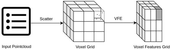
Figure 2.
Input LiDAR pointcloud voxel-wise processing. After scattering all points into corresponding cells, a VFE network yields the initial feature vector for each voxel separately. The dense nature of Voxel Feature Grid (even if filled with zeros when the voxel is empty) enables further layers to be processed in a convolutional manner.
Additionally, 2D convolutions are widely used in an image processing domain, and this approach to pointcloud transformation enables the rest of the network architecture to be based on proven vision solutions. In particular, a Single Shot Detector (SSD) such as YOLO [16,17,18,19] can be adapted as a fast and reliable method. In a single feed-forward inference, it predicts objects as a grid output, where all detections in a scene are placed in the corresponding grid cells. Different grid sizes and related anchor boxes provide results on various object size scales, and with either one-hot class vector encoding or multiple prediction heads, the model can predict objects of different classes at once. Although the mechanisms mentioned boost model performance, they pose a challenge when it comes to adapting explainable AI methods, such as Grad-CAM, to those architectures.
Voxel-wise LiDAR pointcloud processing also has a significant drawback, which is a sparsity of transformed data. LiDAR detections, scattered around a rigid voxel grid, fall only into a small percentage of the voxels, and the rest of them remain empty. During training on such sparse voxel features, a neural network parameter convergence is influenced by uneven spacial data distribution, which leads to a decreased performance and anomalies in results. To address this problem, researchers in the LiDAR depth-completion domain proposed the novel Sparsity Invariant Convolution [20], shown in Figure 3. In principle, the convolution operation remains the same, but an additional mask is used to keep track of empty inputs, which are omitted during the application of a filter. Moreover, based on the mask, each utilized component of the convolution sum is weighted, so that the result of the operation has same significance, regardless of the number of non-empty inputs. Sparsity Invariant Convolution became new standard for depth-completion methods [21,22,23], as it drastically improves sparse LiDAR pointcloud processing. In addition to a performance boost, it also affects intermediate neural network feature maps, which are used in XAI Class Activation Maps method, and addressing data sparsity might also improve visualization quality.
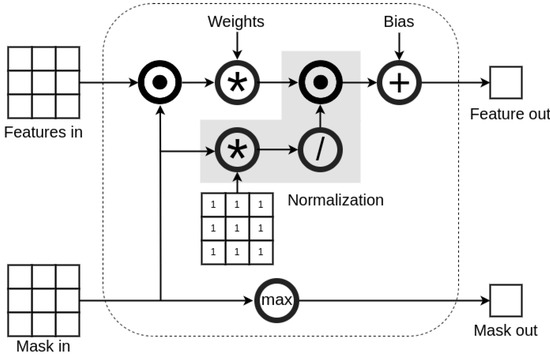
Figure 3.
Sparsity Invariant Convolution operation diagram. Layer dedicated to handle convolution with significantly sparse input data. It uses mask, propagated along the features, to keep track of empty inputs deep within the network structure, which are then mask before multiplication with layer trainable weights. Additionally, results are scaled accordingly to mask values before adding a bias.
3. Proposed Approach
Processing a LiDAR pointcloud with a neural network, as stated in Section 2, requires architectural solutions specific to that type of datum. On the other hand, such changes significantly affect the Grad-CAM method application. In order to understand those problems, in this section we will present the model used to detect objects in LiDAR pointcloud and compare original Grad-CAM with our approach.
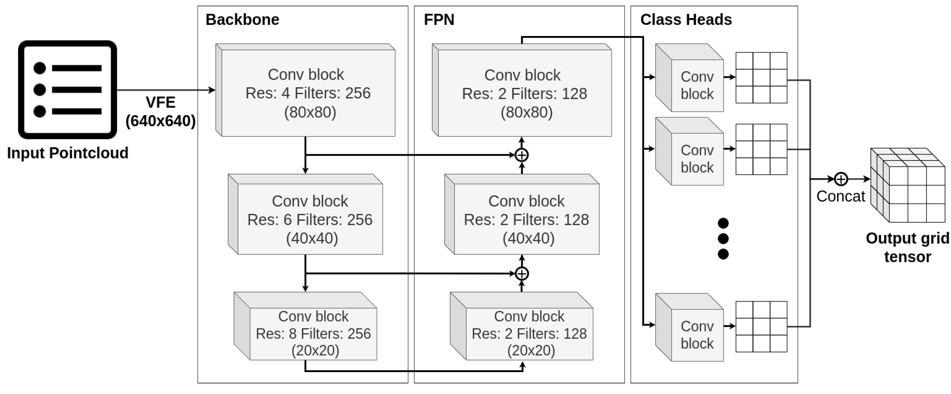
Our proposed LiDAR object detection model is a fully convolutional architecture (Figure 4), that utilizes common mechanics such as residual blocks and skipped connections in a U-shaped network structure, similar to vision models. Gradient-based methods could be applied to this part of a model as they are. The main challenges are posed by the input and the output layers, specific to processing pointcloud data.
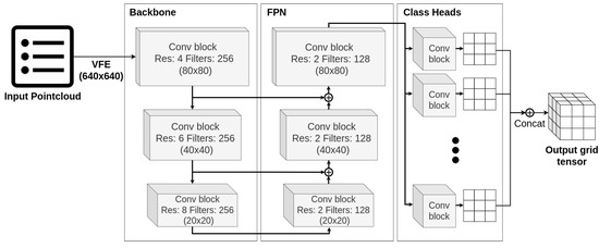
Figure 4.
Proposed object detection LiDAR network architecture. Input pointcloud is processed voxel-wise by VFE block. Then, Backbone and FPN convolutional blocks form a U-shaped core network. Lastly, per class prediction heads yields output grids, which are concatenated into an output tensor.
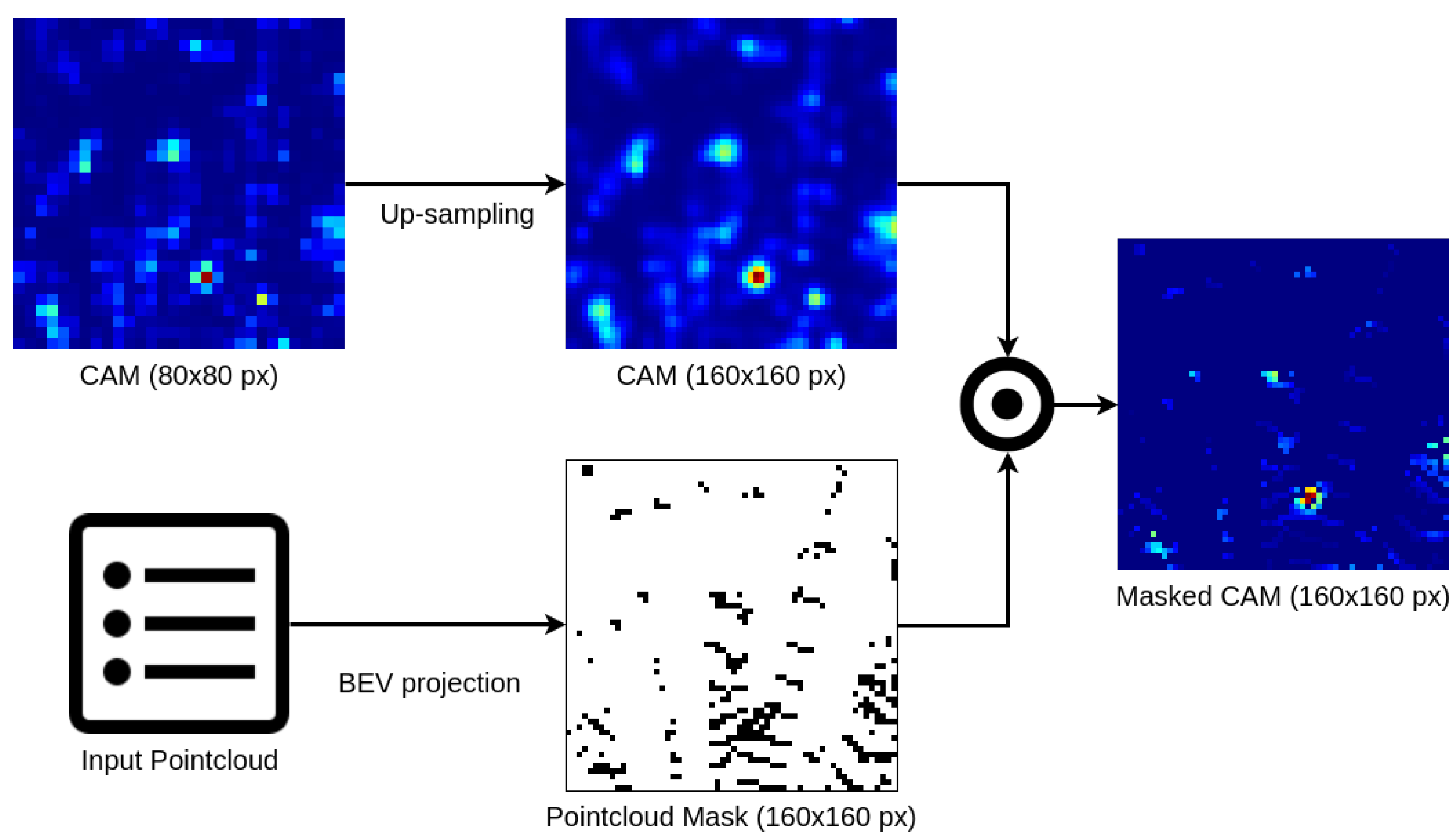
In order to handle the input data, we apply a voxelization method, assigning each detection point to a corresponding voxel and calculating the voxel features based on their content. Then, stacking voxels along z-axis is performed to reduce tensor dimensions. All those operations enable middle layers to process data in a 2D convolutional matter, at a cost of losing pointwise information inside voxels as well as spatial relations along vertically stacked voxel feature vectors. The consequences of these simplifications affect Class Activation Maps creation, as their domain will be a two dimensional, birds-eye view (BEV) perspective with a grid resolution the same as voxel grid at target convolutional layer. To mitigate the effect of a mismatch between 3D pointcloud data and 2D CAMs, we propose a fused visualization method (Figure 5). The method is based on an input pointcloud mask, created by casting each point into a BEV with a resolution significantly higher then a CAM size. It is then applied to CAMs by up-sampling them with cubic interpolation and element-wise multiplication with the mask values. This results in high resolution BEV heatmaps with considerably more detailed information around actual LiDAR readings. The size of the mask affects the outcome of such enhancement, thus we describe experiments with different mask resolutions in a following section.
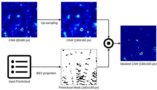
Figure 5.
Masking CAMs with input pointcloud data is performed by casting LiDAR detections onto a dense BEV grid and multiplying the mask with an up-sampled CAM. The operation results in a high resolution heatmap with meaningful values only near actual inputs.
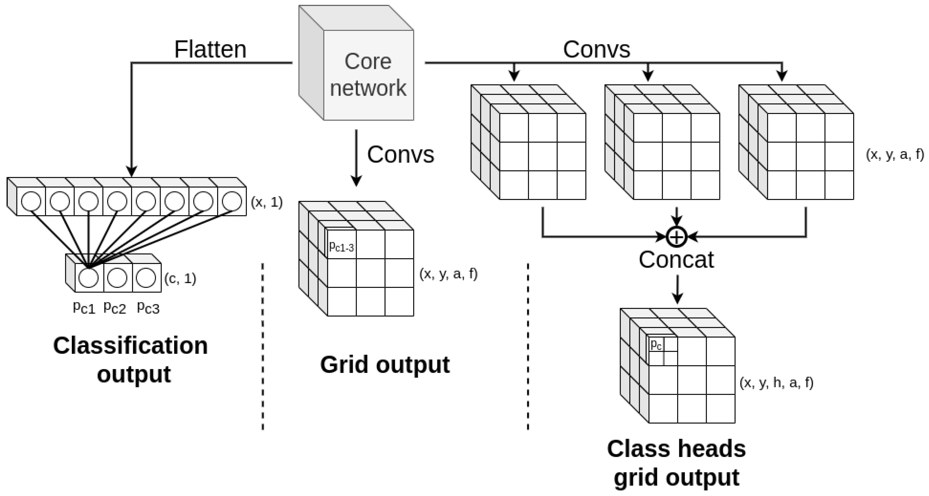
Another area in which adapting a Grad-CAM method to the pointcloud processing model poses a challenge is the output of the network. Arguably, it could have the single greatest effect on the final CAMs result, as the output and related class scores are fundamental components of calculating activations weights via the backpropagation of its gradient to a target activation layer. Due to the model’s purpose and architecture solutions connected to object detection in the form of a single shot detector (SSD), the prediction format is vastly more complex than in a simple classification problem, as illustrated in Figure 6.

Figure 6.
Comparison between different types of model outputs. The classification network outputs a vector of class probabilities, which could be used as a class score as is. The grid tensor output is a more complex structure with four dimensions (x, y, anchors, and features), where class probability values are embedded into feature vector along the fourth dimension. The multi-head output for each class is similar to the grid tensor, but due to the concatenation of all heads it has one additional head dimension (x, y, heads, anchors, and features).
The main goal of processing output in a context of a gradient-based XAI is to obtain a class score value. In an original Grad-CAM use-case for classification problem, the output of the model is a vector with probability predictions for each class. The class score value is the element of this vector under the index corresponding to a given class. In comparison, the SSD object detection model output is a multi-dimensional tensor, where the first two dimensions correspond to the 2D grid of cells that the whole region of interest is divided into. An optional third dimension represents anchor boxes of different sizes, if a model uses them. The last dimension is a per-cell (or anchor) vector of predicted feature values. This multi-feature prediction vector typically consists of fields such as objectiveness score, object position within a cell, object size, and classification probabilities for each class. In this most common output format, we propose the calculation of the class score value using the following formula:
in which the final class score is a sum of class probability predictions of every cell in the output grid along first two spatial grid dimensions , as well as optional anchor dimension a. Additionally, cells are filtered by predicted objectiveness score , which needs to be higher then a certain threshold in order for a cell to be taken into consideration.
Multi-class prediction in SSD models can be also achieved with a different approach. In the method above, we assumed a single prediction output, with a class encoded in a probability vector in every cell. Alternatively, a multiple class prediction mechanism could be embedded into a network structure. At some point, near the output layer, the main processing path branches into several identical prediction heads, one for a single class. Predictions from each head come in a form similar to the previously discussed grid with the exception of a missing classification probability vector in the features. The classification is no longer required due to the fact that, as a result of a training process with class labels properly distributed to corresponding heads, each of them specialize in detecting one particular class exclusively. Dividing the model output into several class-oriented heads could improve model performance, as convolutional filters are optimized separately for each type of objects. It also enables the possibility to define per-class anchor boxes. On the other hand, changing the output format, in particular adding new head dimensions, which constitutes merged head outputs for a single tensor prediction, as well as removing class probability features, affects class score calculation. In case of a multi-head output architecture, we propose following class score formula:
in which, as previously, we sum every cell score along , but for the head dimension h we filter only the ones corresponding to a given class . Addressing the problem of missing class probability features, we decided to use the objectiveness score , as it substitutes classification probability if a given head yields only this particular class of object.
Class score value is an initial point of a backpropagation algorithm which returns gradient values for a chosen convolutional layer with respect to the score. Those gradients in a Grad-CAM technique are the basis for obtaining weights of activations at a given layer. There are a couple of verified methods to calculate the weights out of the gradient values. In our adaptation to LiDAR pointcloud data, we tried to use both original Grad-CAM and Grad-CAM++ formulas, and both of them show satisfactory results. As the original method is very elegant in its simplicity, yet sufficient for our needs, we decided to use it as is, without altering it in any way.
A separate architecture solution is used for detecting objects of the same class which differ significantly in size in selected region of interest (i.e., due to sensor perspective). For this problem, the model outputs several independent tensors, which vary in grid sizes, imitating diversified scales of detections. Creating a single CAM in the case of a multi-scale model is quite problematic as outputs, activations, and gradients tensors are different in size for each scale as well. We suggest applying Grad-CAM methods to every scale independently, as discussed above for single-scale models. The independent visualizations for each scale could prove to be more informative then a one-merge heatmap. Moreover, rescaling and merging CAMs is a much more approachable task in the image domain, thus when a single map is required for multi-scale model, we advise to create CAMs for each scale and merge them as images. The multi-scale model is not the case in our solution, as objects in BEV perspective remain the same with respect to the size, regardless of their relative position to the LiDAR. During our research, we did however try multi-scale CAMs generation for a vision model (Figure 7), where the same object could have a different size (and best matching anchor) depending on the distance from the camera.
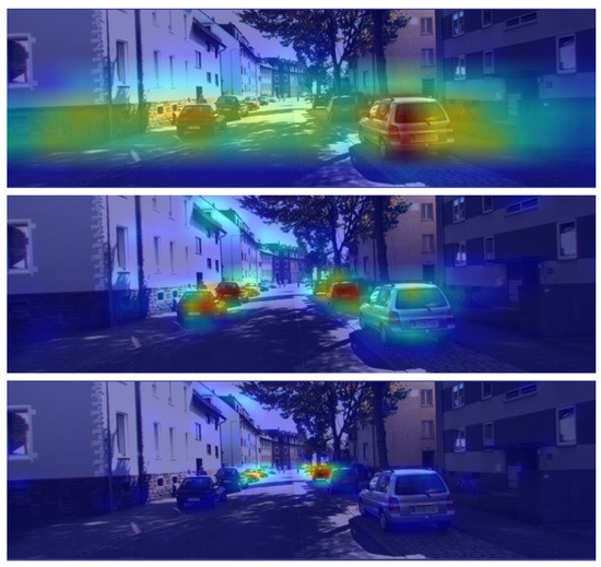
Figure 7.
We apply the proposed Grad-CAM method to a vision object detection network with a multi-scale output grid. From top to bottom there is large, medium and small scale output CAM visualization for a class. Results show distinct distances of detected objects from camera sensor at different scales. Combining CAMs and known labels, we can assign detection ranges for each output to better understand the model.
A previously proposed solution applies to one out of two parts of the Grad-CAM method, namely weights of the activations. During our research we noticed that, despite some of the CAMs generated with the use of our adapted technique looking accurate, in other cases they are influenced by some kind of noise. After further investigation, it turned out that even though gradient-based weights are properly calculated, the most relevant activations themselves are distorted, mainly in the parts of a grid where no input data are present. We started to examine the root cause, which we believe is a sparse nature of LiDAR pointcloud after a voxelization process. Due to the fact that a voxel-wise processing is an inseparable step of our network architecture, as well as the vast majority of LiDAR object detection models, we want to address this issue without discarding it altogether. We searched for a solution to the sparsity problem, which led us to incorporating Sparsity Invariant Convolution throughout our model in the place of ordinary convolutional layers. As a result, activations are free of the noise generated by empty input data, which significantly improves the quality of final CAMs, as we show in the next section.
4. Experiments and Results
Explainable AI methods, such as Grad-CAM, show the reasoning behind given model predictions which are more understandable to humans. In order to present our approach and results for a LiDAR pointcloud processing architecture, we first needed to train the actual model that performs the object detection task on the data. We decided to work with a popular, open-source autonomous driving dataset called KITTI [8]. The sensor suite of the car used to collect it consists of two cameras for stereo vision, a rotating LiDAR sensor mounted on top of the roof and a set of 2D and 3D human-annotated labels for different classes of objects present in the scene. We divided the whole dataset into three subsets: training, validation, and testing, which consist of 4800, 2000, and 500 samples, respectively. We trained the architecture proposed in a previous section for 250 epochs on the training dataset, monitoring the progress with a use of validation examples. All presented results, as well as performance metrics, were calculated on test samples. After the training, we verified our solution using a popular object detection metric called Mean Average Precision (mAP). Our model achieves a mAP score of 0.77 and 0.76 for car and track class, respectively, as well as a mAP of 0.53 and 0.51 for pedestrian and bicycle class, respectively. Such scores place it in the middle of the official KITTI leader-board for the BEV object detection task. As the purpose of this work is to adapt the Grad-CAM method, and not to obtain highest state-of-the-art score in an object detection, we believe the performance of the model to be satisfactory enough to carry on with it.
Our initial experiment concerned applying the Grad-CAM method to a LiDAR pointcloud processing network with a minimal modifications needed for it to work when compared to original vision application. The activations are obtained during feed-forward inference, so the only missing element to create CAMs are the weights. In order to determine the activation weights, we needed to propagate gradients from the class score value to a target convolutional layer. We used our proposed algorithm described before for the multi-head network output to accumulate a class score across whole prediction grid, then fed it into a backpropagation algorithm. Then, with a use of an original Grad-CAM formula, we extracted weights from the gradients. We tried different target convolutional layers to calculate CAMs. After checking several possible candidates, the best visual results came from the class head layers near the prediction output. The first Grad-CAM results for pointcloud data (Figure 8) look appropriate, in a sense that the created map highlights objects in a scene, which proves our method of accumulating a class score across output grid and generating weights captures activations responsible for yielding object predictions. On the other hand, we found them inaccurate detail-wise compared to the sensor resolution and also burdened with significant noise.
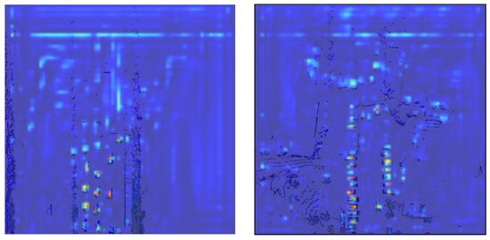
Figure 8.
Original Grad-CAM adaptation results for LiDAR pointcloud with the use of our proposed class score calculation for an object detection grid tensor output. Objects (cars) are highlighted properly, but we could observe noise in generated CAM. The level of CAM detail is also low when compares to casted LiDAR detections (dark blue) resolution.
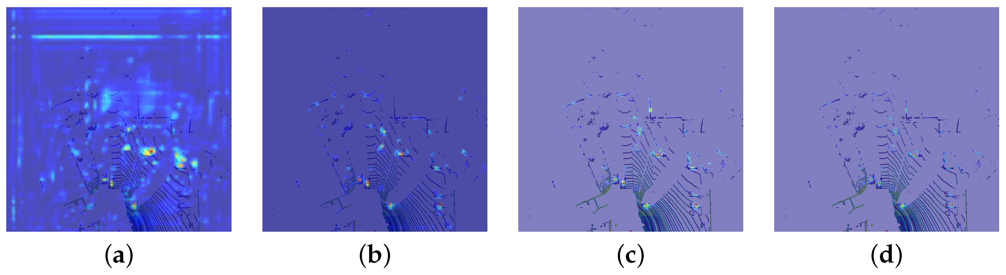
Addressing the low resolution problem, in our next attempt, we applied a pointcloud-based mask to a CAM visualization in order to extend the level of detail of the result. The chosen activation layer, as well as the generated CAM, has a resolution of , whereas pointcloud BEV projection could be performed with any given grid size. The pointcloud overlay in the presented results is , which corresponds to a 12.5 cm by 12.5 cm cell represented by a single pixel. Therefore, we conducted experiments with pointcloud binary masks of sizes ranging from to (Figure 9). Our main observation regarding pointcloud masks is that, at higher resolution, CAM are extremely filtered to the LiDAR detections, so the integrity of object instances is lost and the visualization looks too grained and thus illegible. On the other hand, a resolution of yields no improvement to the precision. Hence, we decided to use a mask resolution, as it compromises between readability and the level of detail. There are also other, not as explicitly visible advantages of applying such a mask. In the CAM domain, before visualization, the values from each weighted activation are genuinely small and the normalization process is needed to visualize them as an 8-bit image. As the masking is done prior to it, some parts of the activation are masked and not taken into account during a normalization, which results in a wider spectrum range for relevant CAM values. This could be observed in different mask visualization backgrounds as well as near highly confident detections.
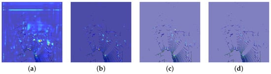
Figure 9.
In this figure, we compare different input pointcloud mask resolutions assumed while casting points to BEV: (a) no mask, (b) 80, (c) 160, and (d) 640 pixels. Without a mask, the generated CAM is noisy and imprecise. Application of masks filters the noise and increases the level of detail near the input pointcloud data. However, at higher mask resolutions, CAMs become too grained and thus not valid for a human visualization.
Although using a pointcloud mask also filters out the vast majority of noise in generated CAMs, we do not consider it a solution to that problem. When part of a CAM which is significantly corrupted by noise happens to be covered with LiDAR detections (i.e., trees, bushes) as well, then the masking process would not filter it properly. We checked our implementation of calculating the class score, gradient backpropagation, and weights generation, but the noise problem is not always present, and some of generated CAMs are clear. Therefore, we searched for the root cause in the last major element of CAMs creation, which is inferred activations.
In Figure 10, we show a visualisation of a single activation which, based on gradient values, has a significant weight for the CAM creation. Even though the activation values in the middle look vital for the CAM, the noise in the corner outbalances the rest and the outcome is corrupted. We found lots of cases similar to presented one, and the common aspect of the noise is that it appears in a part of the grid where input data is empty due to the sparse nature of voxel-wise pointcloud processing. Addressing this problem poses a challenge, as activations are obtained during feed-forward inference, which depends largely on the network structure and trained weights. For our final experiment, we changed every convolutional layer in our network architecture to a Sparsity-Invariant Convolution with similar parameters and retrained the whole model. Then, we repeated the activation analysis and found significant improvement over the previous model. Additionally, in Figure 10, we present the exact same sample generated with the similar CAM method, but with the use of a different model. Sparsity Invariant Convolutions drastically reduced the noise generated by empty input data, and the resulting CAM is clearer with improved distinction of important regions.
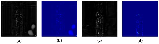
Figure 10.
Activation (a) and related CAM (b) were generated with a model with normal convolutions, whereas for the exact same sample activation (c) and related CAM (d) were obtained with a model with Sparsity Invariant Convolutions instead. We can observe the noise in the former activation map, which also corrupts generated CAM. The latter example shows that the sparsity invariant operation surpasses the previous method, especially when it comes to empty input cells. As a result, the generated CAM is concentrated on actual detections with a higher confidence.
Combining all of our proposed solutions for Grad-CAM adaptation to LiDAR pointcloud network, in Figure 11 we demonstrate the final result of our work. We use voxel-wise processing and 2D Sparsity Invariant Convolutions to infer model output, as well as intermediate activations from a target convolutional layer. Then, based on the proposed algorithm, we determine the class score from a multi-head, multi-feature model output tensor. With backpropagation, we find gradients for target layer with respect to the class score, and then calculate the activation weights for CAMs creation. Finally, we fuse obtained CAMs with a LiDAR pointcloud mask to enhance them with a higher level of detail. The final result is a high resolution, detailed heatmap of input significance for an object detection task on a LiDAR sensor pointcloud, which is also free of any undesirable noise that could disrupt human visual analysis. In Figure 12, we compare results of Grad-CAM visualization for different classes of LiDAR object detections, namely car, track, bicycle, and pedestrian predictions.
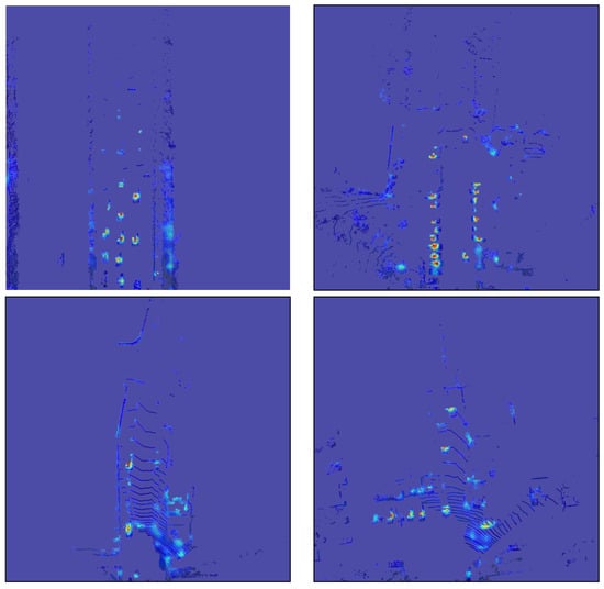
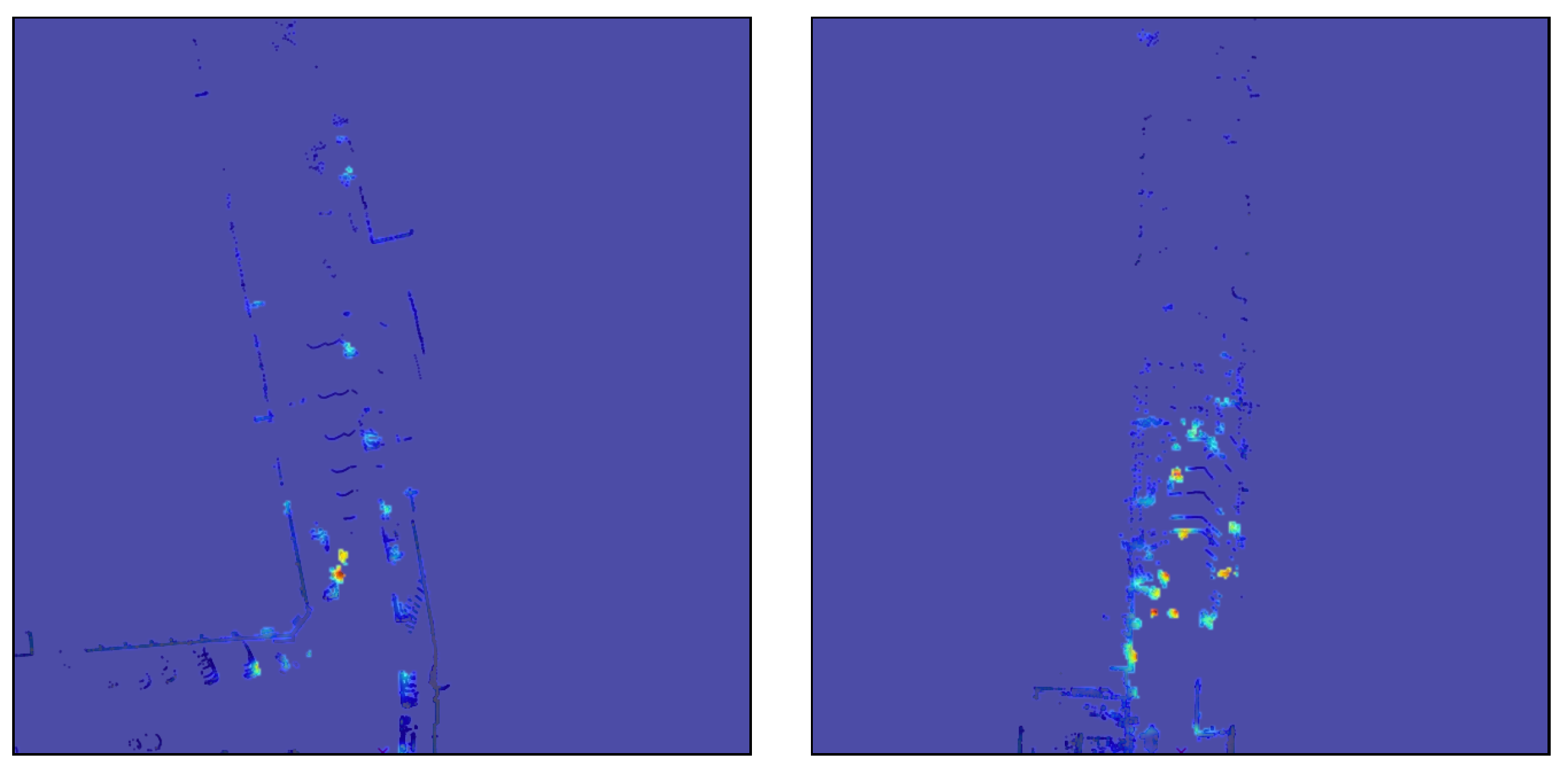
Figure 11.
Final Grad-CAM adaptation results for a LiDAR pointcloud object detection network. Combining all of our experiments and findings, we were able to create our final pipeline for CAMs creation. This results in a high resolution, clear, and free of noise CAM heatmap that highlights important areas in an input pointcloud overlay.
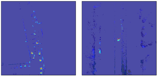
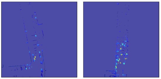
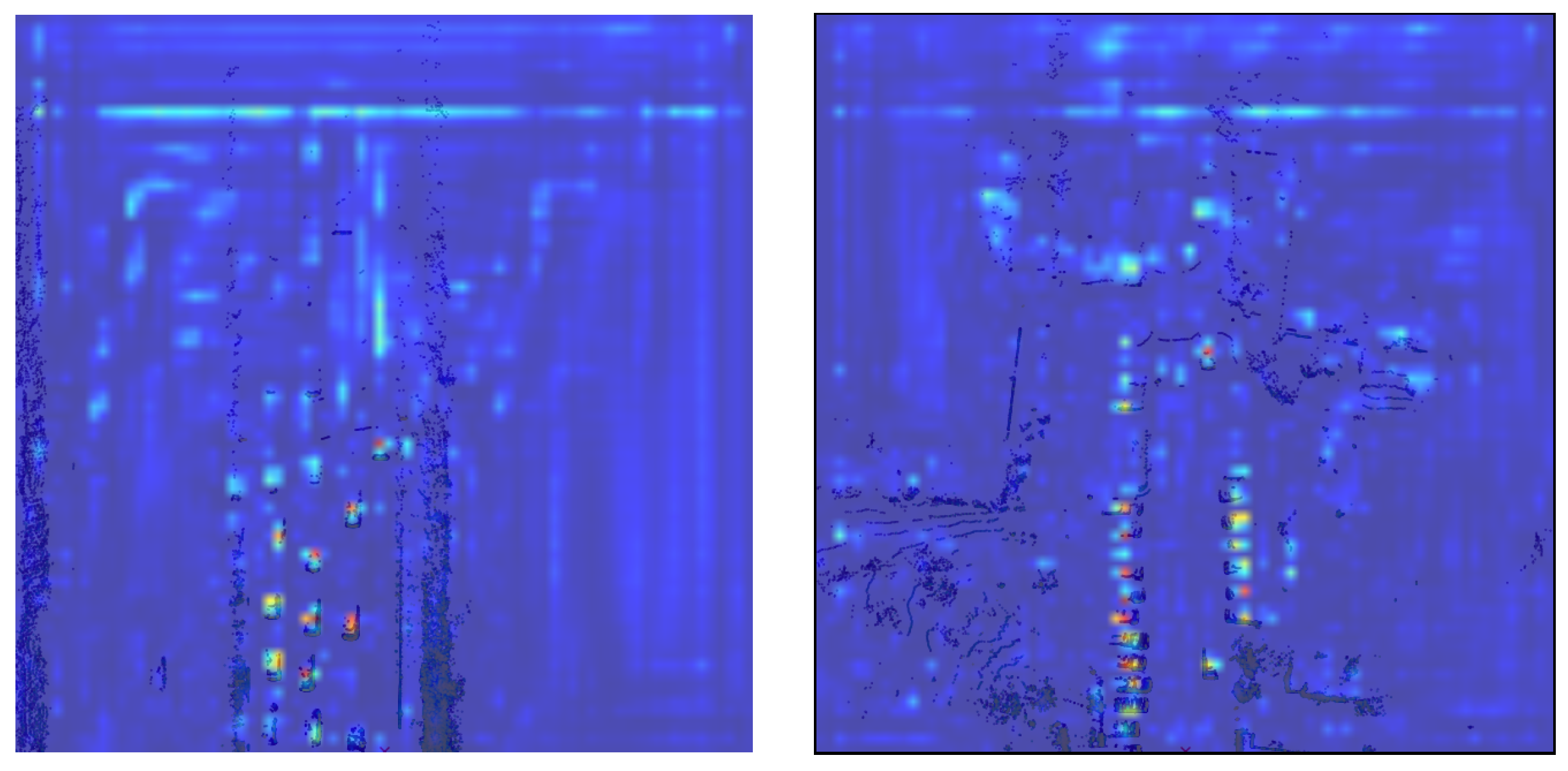
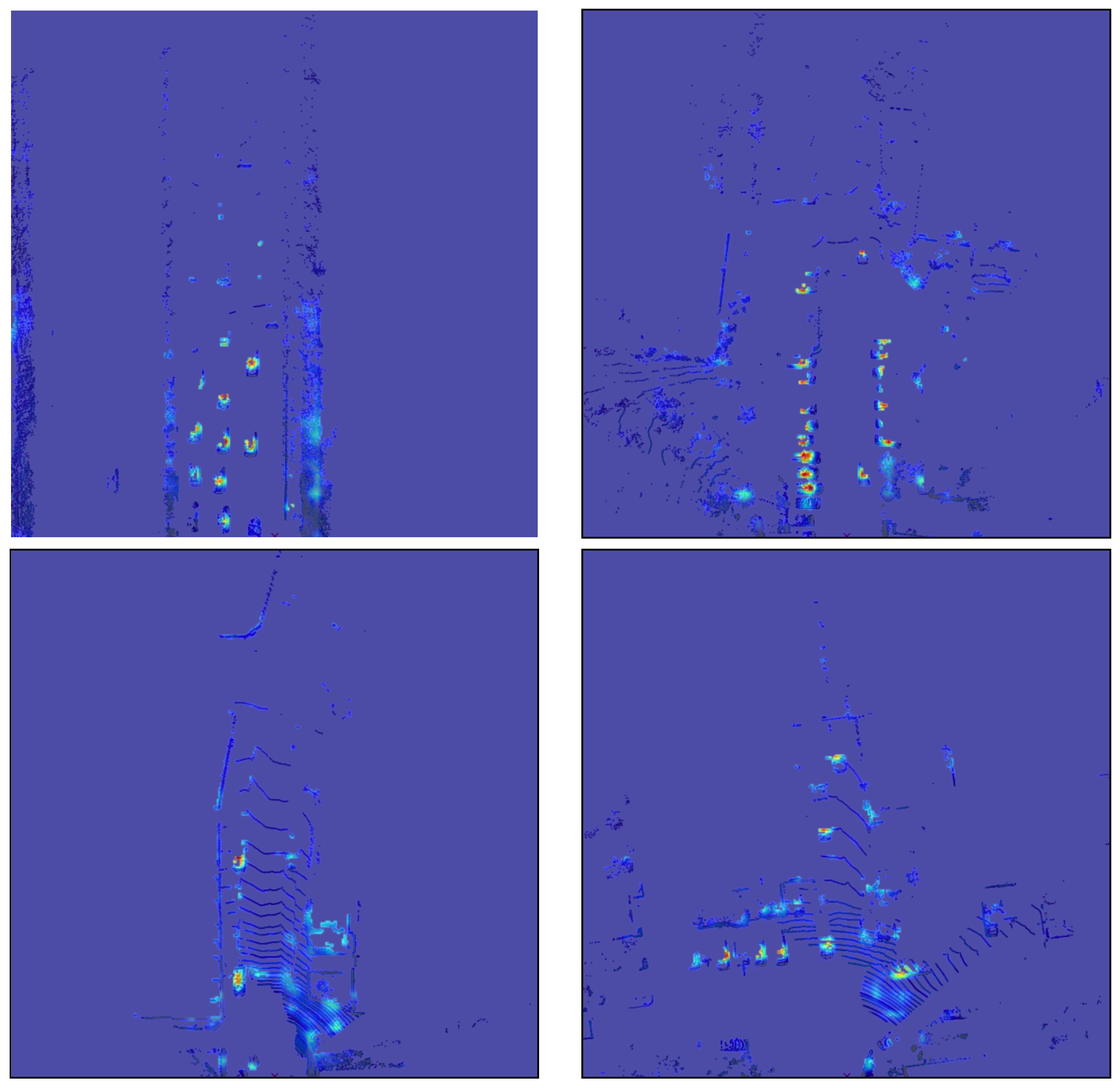
Figure 12.
Comparison between results for different classes. The top left and bottom left Grad-CAMs are generated for the same scene, but for a car and bicycle class, respectively. The top right image represents a track class detection interpretation. The bottom right shows a dense urban scenario with a pedestrian detection heatmap.
5. Conclusions
In this article, we presented an adaptation of a gradient-based XAI method called Grad-CAM from an original camera image domain to a LiDAR pointcloud data. Our proposed Grad-CAM solution for processing a new data format, as well as a unique network structure used in LiDAR object detection architecture, achieves said task with most satisfactory results. Using our method, researchers could visualize pointcloud neural network results with respect to the input data to help understand and explain the decision-making process within a trained model, which was previously limited to the image networks domain. Additionally, such visual interpretation could help during the development process, as it highlights problems in a way that is easy to understand by a human.
We encountered one such problems during this research, namely noise in generated CAMs. With the use of activation heatmap visualization, we were able to determine the sparse data issue after voxelization and correct it with Sparsity Invariant Convolutions to obtain even better results. The drawback of this adjustment is the need to replace old convolution operations in a network structure and retrain the whole model but, as we have shown, this type of convolutional layer is much more suitable for sparse pointcloud data.
For future work, we would like to investigate the sparse pointcloud data problem even further. Although Sparsity Invariant Convolutions address the problem, they are still processing dense tensors with lots of empty values. An interesting outcome might be derived from using sparse tensors representation with a truly sparse convolution implementation applied to it. The resulting model should also be explainable with our Grad-CAM approach, as long as gradients would propagate back from a class score to a target layer.
Lastly, we presented our adaptation from a camera image domain to LiDAR pointcloud data only. Among automotive sensors, radars are also widely used in production perception systems. Progressively more such systems are being developed with the use of neural networks, which still lack XAI methods such as Grad-CAM. Radar and LiDAR pointcloud data formats differ, but they are more related to each other than to a camera image, thus only moderate changes would need to be performed in order to apply our method to radar networks as well.
Author Contributions
Conceptualization, D.D. and J.B.; methodology, D.D. and J.B.; software, D.D.; validation, D.D.; formal analysis, D.D.; investigation, D.D.; resources, J.B.; data curation, D.D.; writing—original draft preparation, D.D.; writing—review and editing, D.D. and J.B.; visualization, D.D.; supervision, J.B.; project administration, J.B.; and funding acquisition, J.B. All authors have read and agreed to the published version of the manuscript.
Funding
Research is partially funded by Polish Ministry of Science and Higher Education (MNiSW) Project No. 0014/DW/2018/02, and partially by AGH’s Research University Excellence Initiative under project “Interpretable methods of process diagnosis using statistics and machine learning”. and within the scope of NAWA Polish National Agency for Academic Exchange project “Science without borders. Establishing the framework for the long-term international cooperation of academic environments”. contract no. PPI/APM/2018/1/00049/U/001.
Institutional Review Board Statement
Not applicable.
Informed Consent Statement
Not applicable.
Data Availability Statement
Not applicable.
Acknowledgments
Work was carried out in cooperation of Aptiv Services Poland S.A.—Technical Center Kraków and AGH University of Science and Technology—Faculty of Electrical Engineering, Automatics, Computer Science and Biomedical Engineering.
Conflicts of Interest
The authors declare no conflict of interest.
References
- Guidotti, R.; Monreale, A.; Turini, F.; Pedreschi, D.; Giannotti, F. A Survey of Methods for Explaining Black Box Models. ACM Comput. Surv. 2018, 51, 1–42. [Google Scholar] [CrossRef] [Green Version]
- Adadi, A.; Berrada, M. Peeking Inside the Black-Box: A Survey on Explainable Artificial Intelligence (XAI). IEEE Access 2018, 6, 52138–52160. [Google Scholar] [CrossRef]
- Samek, W.; Wiegand, T.; Müller, K. Explainable Artificial Intelligence: Understanding, Visualizing and Interpreting Deep Learning Models. arXiv 2017, arXiv:1708.08296. [Google Scholar]
- Omeiza, D.; Webb, H.; Jirotka, M.; Kunze, L. Explanations in Autonomous Driving: A Survey. IEEE Trans. Intell. Transp. Syst. 2021, 1–21. [Google Scholar] [CrossRef]
- Zhou, B.; Khosla, A.; Lapedriza, A.; Oliva, A.; Torralba, A. Learning Deep Features for Discriminative Localization. In Proceedings of the 2016 IEEE Conference on Computer Vision and Pattern Recognition (CVPR), Las Vegas, NV, USA, 27–30 June 2016; pp. 2921–2929. [Google Scholar] [CrossRef] [Green Version]
- Selvaraju, R.R.; Cogswell, M.; Das, A.; Vedantam, R.; Parikh, D.; Batra, D. Grad-CAM: Visual Explanations from Deep Networks via Gradient-Based Localization. In Proceedings of the 2017 IEEE International Conference on Computer Vision (ICCV), Venice, Italy, 22–29 October 2017; pp. 618–626. [Google Scholar] [CrossRef] [Green Version]
- Chattopadhay, A.; Sarkar, A.; Howlader, P.; Balasubramanian, V.N. Grad-CAM++: Generalized Gradient-Based Visual Explanations for Deep Convolutional Networks. In Proceedings of the 2018 IEEE Winter Conference on Applications of Computer Vision (WACV), Lake Tahoe, NV, USA, 12–15 March 2018; pp. 839–847. [Google Scholar] [CrossRef] [Green Version]
- Geiger, A.; Lenz, P.; Urtasun, R. Are we ready for Autonomous Driving? The KITTI Vision Benchmark Suite. In Proceedings of the IEEE Conference on Computer Vision and Pattern Recognition (CVPR), Providence, RI, USA, 16–21 June 2012; pp. 3354–3361. [Google Scholar]
- Inbaraj, X.A.; Villavicencio, C.; Macrohon, J.J.; Jeng, J.H.; Hsieh, J.G. Object Identification and Localization Using Grad-CAM++ with Mask Regional Convolution Neural Network. Electronics 2021, 10, 1541. [Google Scholar] [CrossRef]
- Cheng, G.; Yang, J.; Gao, D.; Guo, L.; Han, J. High-Quality Proposals for Weakly Supervised Object Detection. IEEE Trans. Image Process. 2020, 29, 5794–5804. [Google Scholar] [CrossRef] [PubMed]
- Laugustin, A.; Canal, C.; Rabot, O. State-of-the-Art Laser Diode Illuminators for Automotive LIDAR. In Proceedings of the 2019 Conference on Lasers and Electro-Optics Europe & European Quantum Electronics Conference (CLEO/Europe-EQEC), Munich, Germany, 23–27 June 2019; p. 1. [Google Scholar] [CrossRef]
- Lee, S.; Lee, D.; Choi, P.; Park, D. Accuracy-Power Controllable LiDAR Sensor System with 3D Object Recognition for Autonomous Vehicle. Sensors 2020, 20, 5706. [Google Scholar] [CrossRef] [PubMed]
- Li, Y.; Ma, L.; Zhong, Z.; Liu, F.; Chapman, M.A.; Cao, D.; Li, J. Deep Learning for LiDAR Point Clouds in Autonomous Driving: A Review. IEEE Trans. Neural Netw. Learn. Syst. 2021, 32, 3412–3432. [Google Scholar] [CrossRef] [PubMed]
- Zhou, Y.; Tuzel, O. VoxelNet: End-to-End Learning for Point Cloud Based 3D Object Detection. In Proceedings of the 2018 IEEE/CVF Conference on Computer Vision and Pattern Recognition, Salt Lake City, UT, USA, 18–23 June 2018; pp. 4490–4499. [Google Scholar] [CrossRef] [Green Version]
- Lang, A.H.; Vora, S.; Caesar, H.; Zhou, L.; Yang, J.; Beijbom, O. PointPillars: Fast Encoders for Object Detection From Point Clouds. In Proceedings of the 2019 IEEE/CVF Conference on Computer Vision and Pattern Recognition (CVPR), Long Beach, CA, USA, 15–20 June 2019; pp. 12689–12697. [Google Scholar] [CrossRef] [Green Version]
- Redmon, J.; Divvala, S.; Girshick, R.; Farhadi, A. You Only Look Once: Unified, Real-Time Object Detection. In Proceedings of the 2016 IEEE Conference on Computer Vision and Pattern Recognition (CVPR), Las Vegas, NV, USA, 27–30 June 2016; pp. 779–788. [Google Scholar] [CrossRef] [Green Version]
- Redmon, J.; Farhadi, A. YOLO9000: Better, faster, stronger. In Proceedings of the 2017 IEEE Conference on Computer Vision and Pattern Recognition (CVPR), Honolulu, HI, USA, 21–26 July 2017; pp. 6517–6525. [Google Scholar] [CrossRef] [Green Version]
- Redmon, J.; Farhadi, A. YOLOv3: An Incremental Improvement. arXiv 2018, arXiv:1804.02767. [Google Scholar]
- Bochkovskiy, A.; Wang, C.; Liao, H.M. YOLOv4: Optimal Speed and Accuracy of Object Detection. arXiv 2020, arXiv:2004.10934. [Google Scholar]
- Uhrig, J.; Schneider, N.; Schneider, L.; Franke, U.; Brox, T.; Geiger, A. Sparsity Invariant CNNs. In Proceedings of the 2017 International Conference on 3D Vision (3DV), Qingdao, China, 10–12 October 2017; pp. 11–20. [Google Scholar] [CrossRef]
- Jaritz, M.; Charette, R.D.; Wirbel, E.; Perrotton, X.; Nashashibi, F. Sparse and Dense Data with CNNs: Depth Completion and Semantic Segmentation. In Proceedings of the 2018 International Conference on 3D Vision (3DV), Verona, Italy, 5–8 September 2018; pp. 52–60. [Google Scholar] [CrossRef] [Green Version]
- Huang, Z.; Fan, J.; Cheng, S.; Yi, S.; Wang, X.; Li, H. HMS-Net: Hierarchical Multi-Scale Sparsity-Invariant Network for Sparse Depth Completion. IEEE Trans. Image Process. 2020, 29, 3429–3441. [Google Scholar] [CrossRef] [PubMed] [Green Version]
- Yan, L.; Liu, K.; Belyaev, E. Revisiting Sparsity Invariant Convolution: A Network for Image Guided Depth Completion. IEEE Access 2020, 8, 126323–126332. [Google Scholar] [CrossRef]


Publisher’s Note: MDPI stays neutral with regard to jurisdictional claims in published maps and institutional affiliations. |
© 2022 by the authors. Licensee MDPI, Basel, Switzerland. This article is an open access article distributed under the terms and conditions of the Creative Commons Attribution (CC BY) license (https://creativecommons.org/licenses/by/4.0/).