
Solar Energy Demand-to-Supply Management by the On-Demand Cumulative-Control Method: Case of a Childcare Facility in Tokyo

Abstract
:1. Introduction

| Type of Renewable Energy | Demand-to-Supply | Overcoming Uncertainties | |||||||||
|---|---|---|---|---|---|---|---|---|---|---|---|
| Solar | Wind | Bio-Gas | Biomass | Supply | Demand | Battery Capacity | Stochastic Model | Forecast-ing | Real Data | Methods | |
| Wichmann et al. (2019) [16] | √ | Energy-oriented lot-sizing and scheduling | |||||||||
| Moon and Park (2013) [17] | √ | √ | √ | Mixed integer programming | |||||||
| Trappey et al. (2013) [19] | √ | √ | √ | √ | Hierarchical learning model | ||||||
| Xydis (2013) [23] | √ | √ | √ | √ | Weibull and Rayleigh probability density function | ||||||
| Jahanpour et al. (2016) [21] | √ | √ | √ | √ | √ | √ | Trigonometric regression model | ||||
| Santana-Vieraa et al. (2015) [25] | √ | √ | √ | √ | √ | √ | Stochastic programming | ||||
| Takanokura et al. (2014) [24] | √ | √ | √ | √ | √ | √ | Newsboy problem | ||||
| Pham et al. (2019) [20] | √ | √ | √ | √ | √ | √ | Stochastic planning model | ||||
| Uhlemair et al. (2014) [18] | √ | √ | √ | √ | Mixed integer linear programming | ||||||
| Rentizelas et al. (2012) [22] | √ | √ | √ | √ | √ | √ | √ | √ | Forward-sweeping linear programming | ||
| This study | √ | √ | √ | √ | √ | √ | √ | On-demand cumulative-control method | |||
- RQ1
- What are the managerial issues including capital investment in a transition to solar power generation in the targeted renewable energy company?
- RQ2
- How was the demand-to-supply balance between the amount of electricity consumption and the amount of on-site solar power generation at the target facility?
- RQ3
- How to operate a battery more effectively by applying a demand-to-supply management developed in production and logistics? Additionally, how was the moving base storage capacity for on-demand DSMM?
- RQ4
- What was the effect of the day of the week, time of day, and weather on the demand-to-supply management in solar-power generation at the target facility?
- RQ5
- How effective are the capacity of the battery and the initial storage in the battery? Moreover, what is the energy storage opportunity loss at that time?
2. Methods
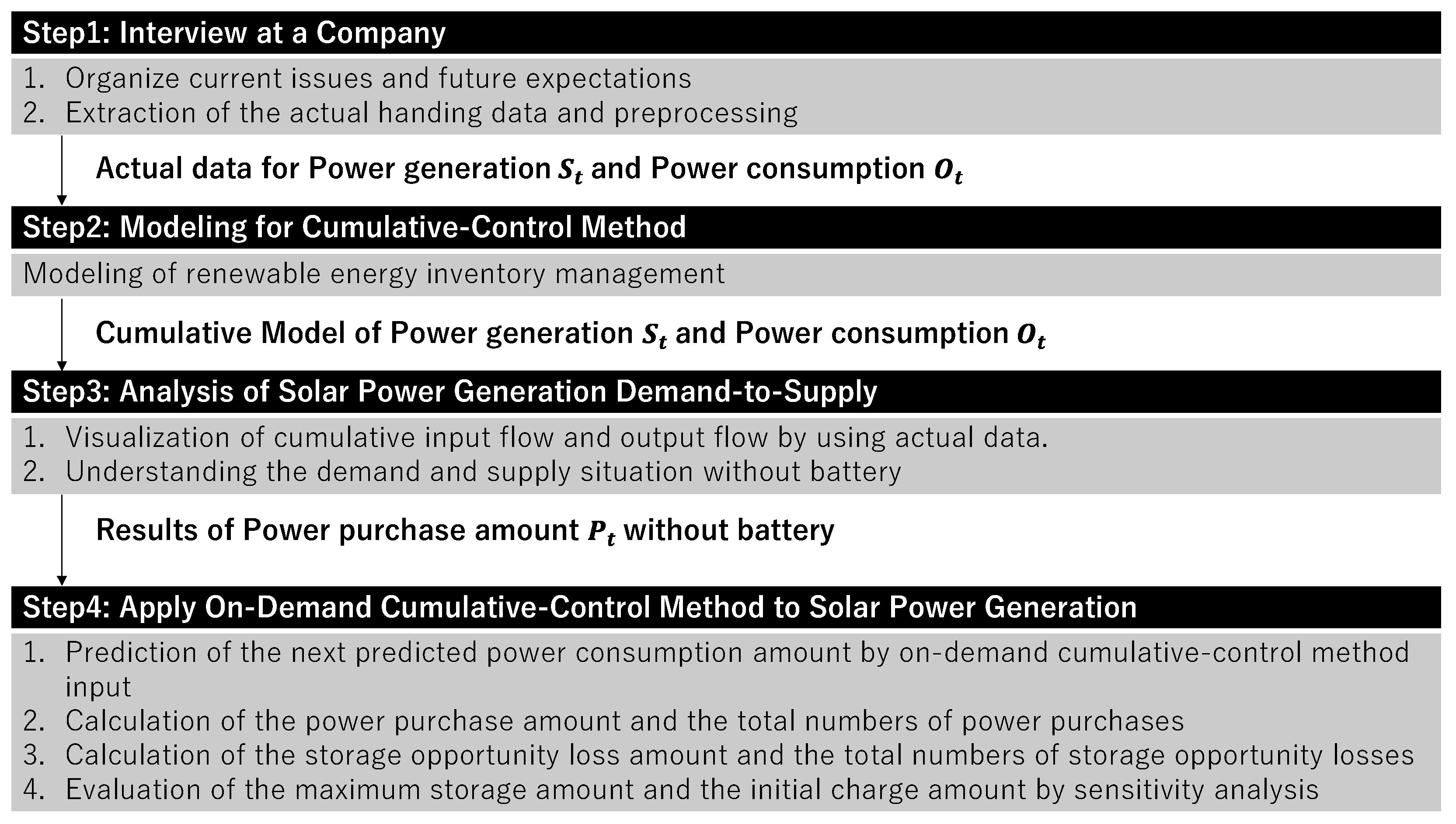
2.1. Procedure
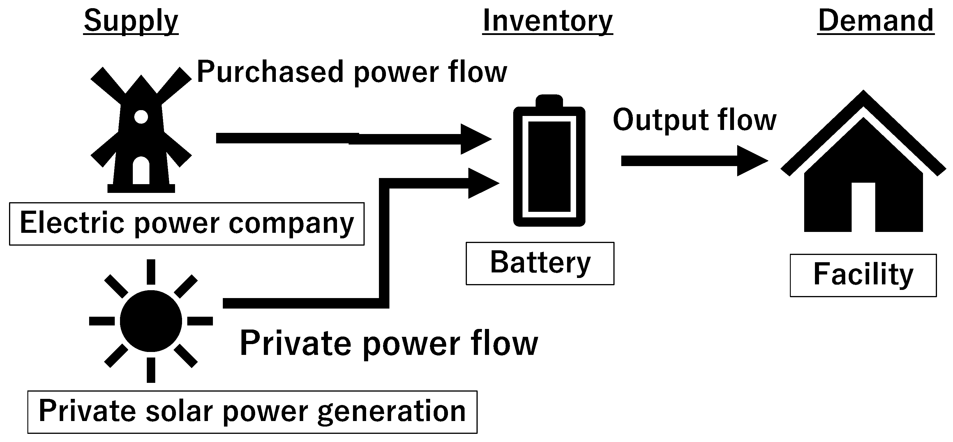
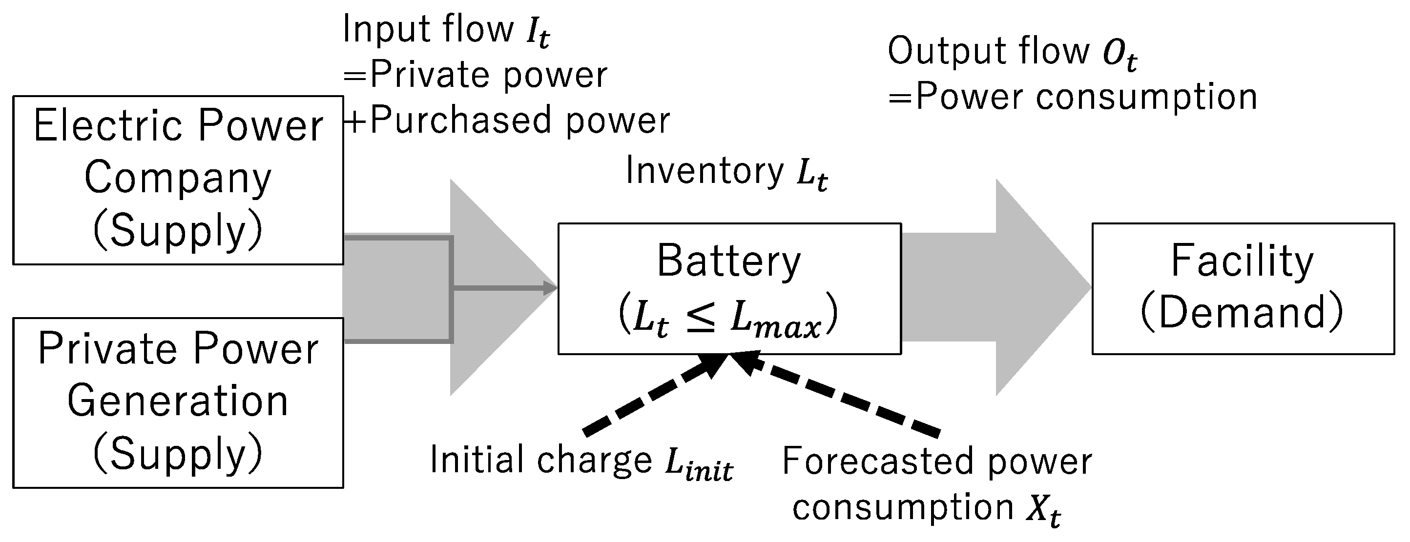
2.2. DSMM Model
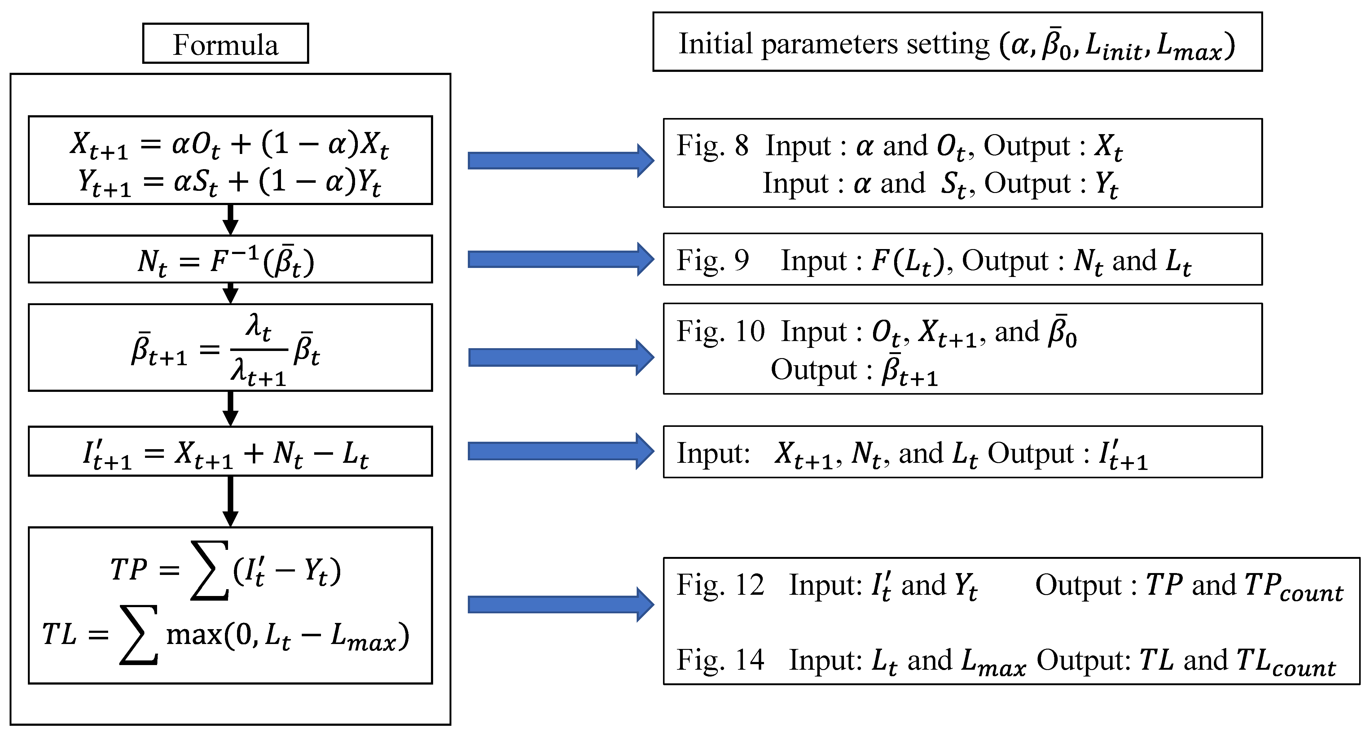
2.3. Cumulative-Control Method
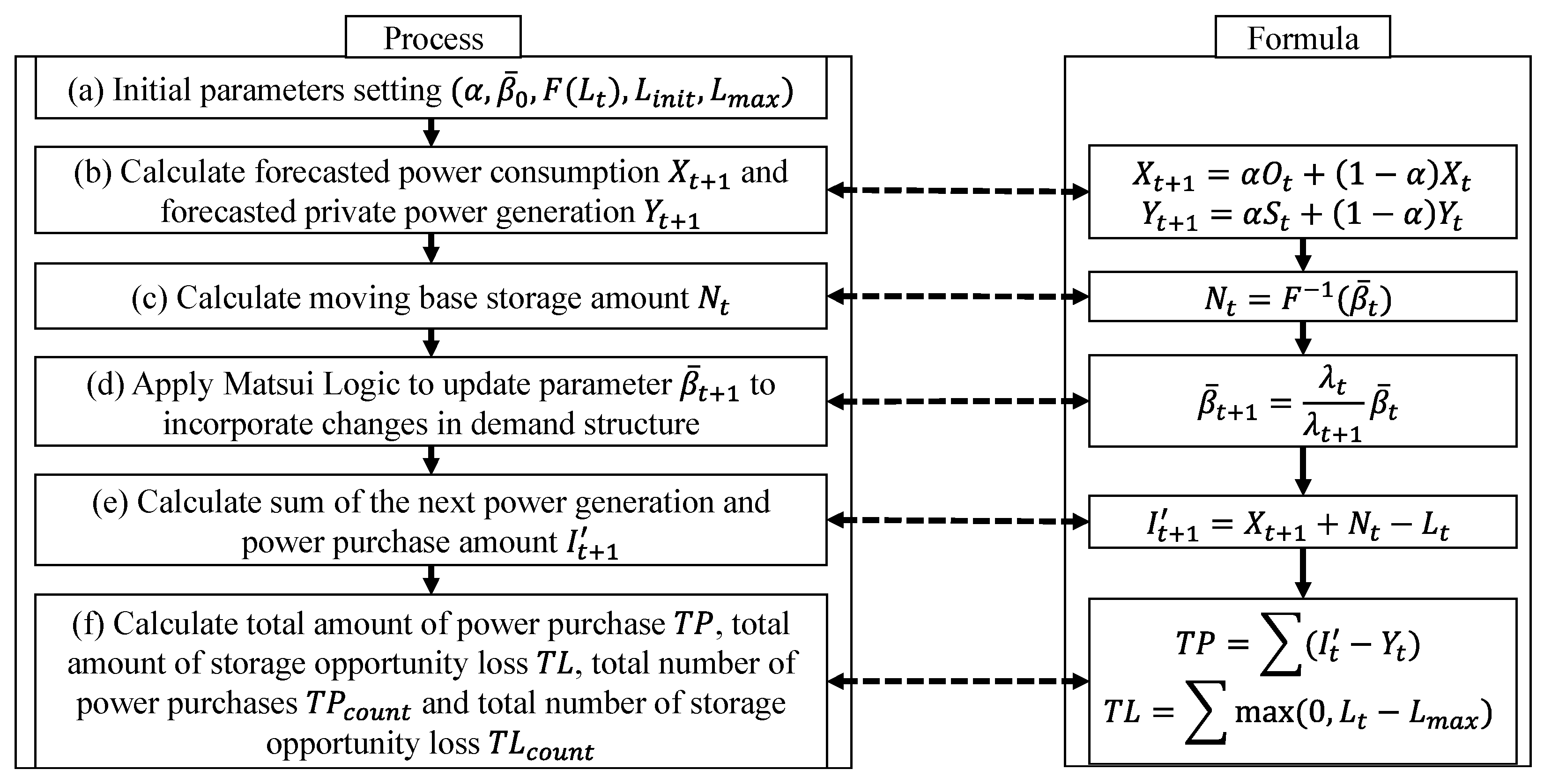
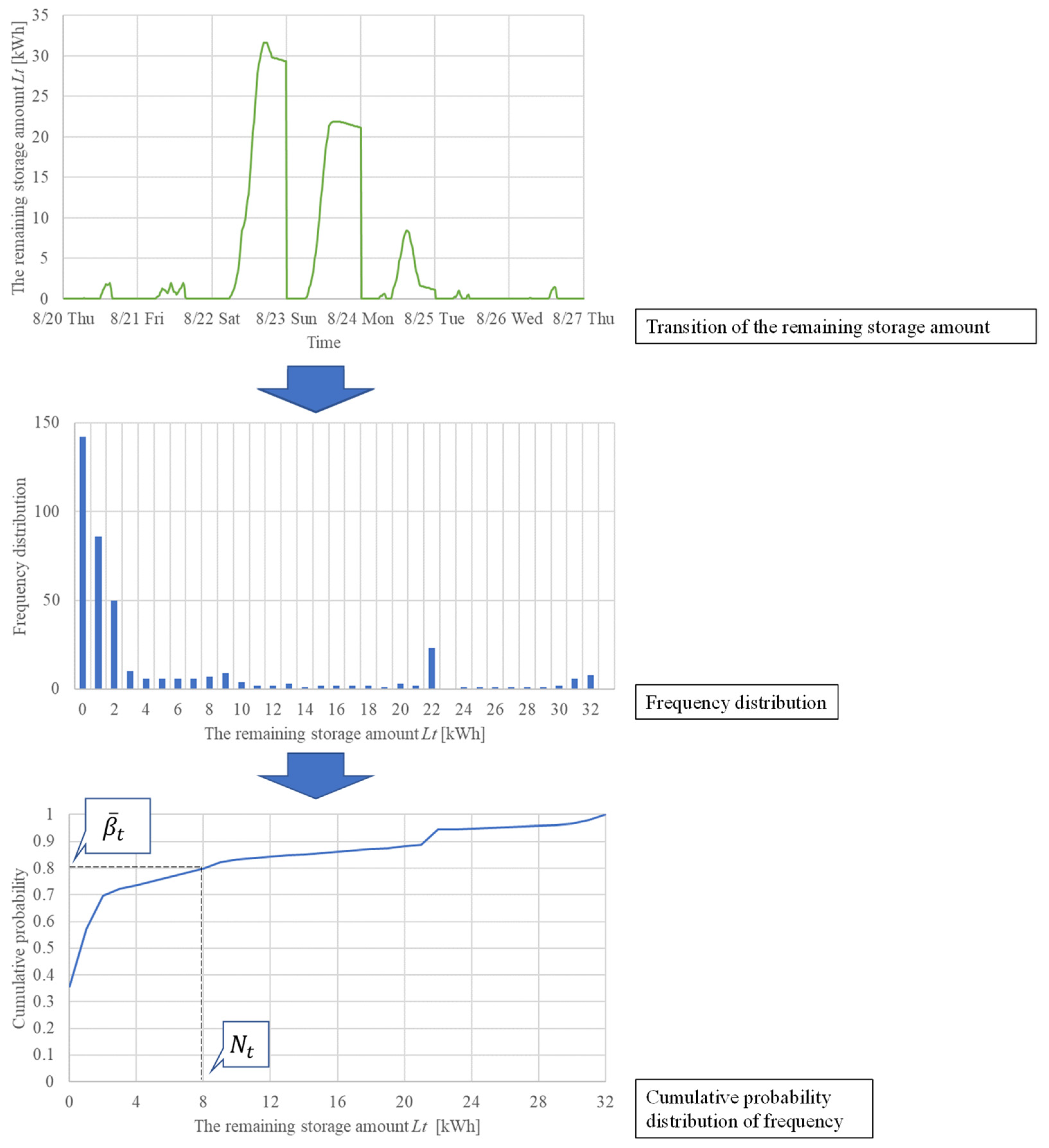
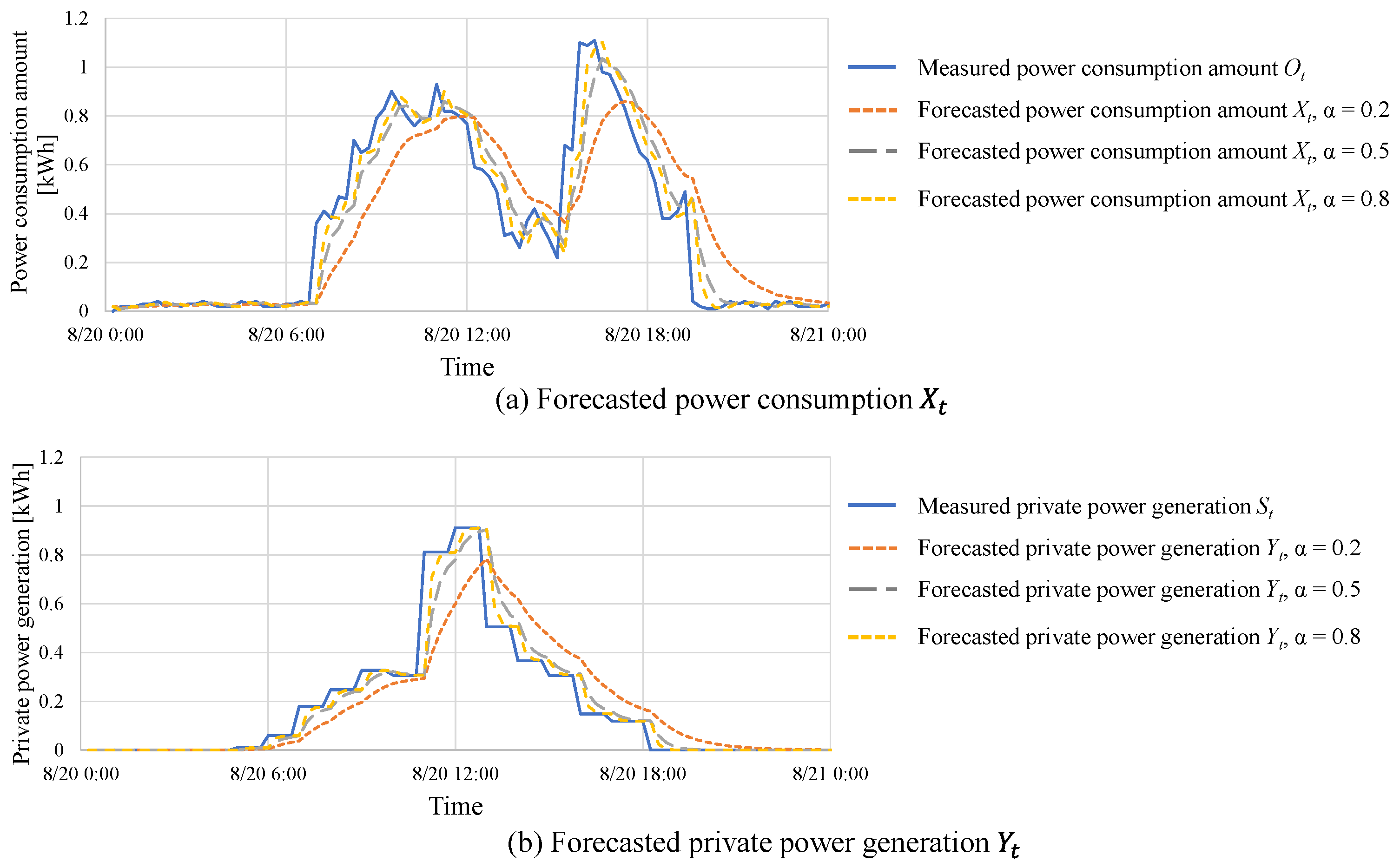
2.4. Application of On-Demand DSMM to Solar Power Generation
3. Results
3.1. Result of Step 1: Company Hearing
3.2. Result of Step 2: Modeling for Cumulative-Control Method
3.3. Result of Step 3: Analysis of Solar Power Generation Demand-to-Supply
3.4. Result of Step 4: Apply on-Demand Cumulative-Control Method to Solar Power Generation
4. Impact of the Proposed Method
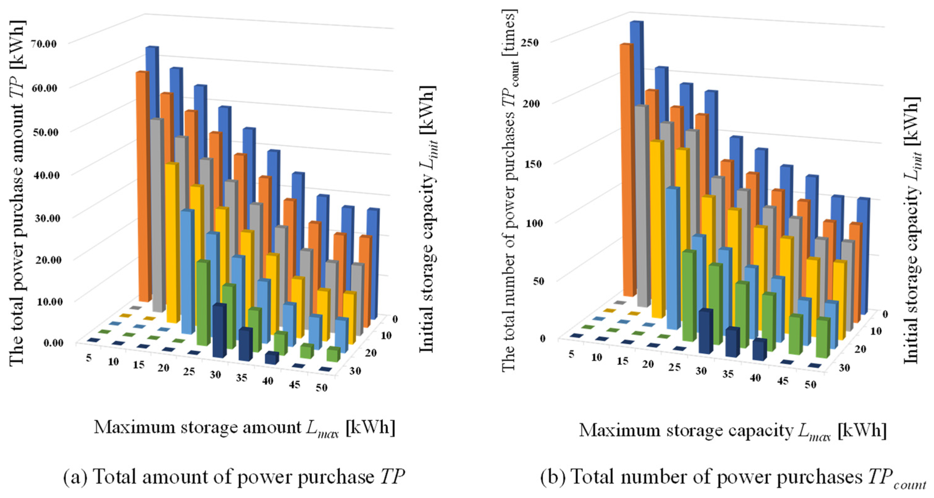
4.1. Maximum and Initial Storage Capacities by Sensitivity Analysis
4.2. Feedback
- We received a positive opinion regarding the sensitivity analysis results of the total power purchase amount TP. They stated that “it is great that even a 20 [kWh] storage battery can achieve the same effect as a 40 [kWh] storage battery depending on how it is used.” This opinion indicates that the modeling of demand-to-supply management of solar power generation using the on-demand demand-to-supply management method was useful;
- We also received a comment stating that “there is a sufficient amount of solar energy falling on the earth. However, we have heard that the technology for fully utilizing this is insufficient, and a storage battery with infinite capacity would be desirable if feasible.” The importance of demand-to-supply management that seeks a realistic storage capacity or initial storage amount was also recognized once again.
4.3. Discussion
- RQ1.
- What are the managerial issues including capital investment in a transition to solar power generation in the targeted renewable energy company?
- RQ2.
- How was the demand-to-supply balance between the amount of electricity consumption and the amount of on-site solar power generation at the target facility?
- RQ3.
- How to operate a battery more effectively by applying a demand-to-supply management developed in production and logistics? Additionally, how was the moving base storage capacity for on-demand DSMM?
- RQ4.
- What was the effect of the day of the week, time of day, and weather on the demand-to-supply management in solar-power generation at the target facility?
- RQ5.
- How effective are the capacity of the battery and the initial storage in the battery? Moreover, what is the energy storage opportunity loss at that time?
5. Conclusions
- The proposed method enables us to pre-process the private power generation data and align them to the same timescale as recorded for power consumption;
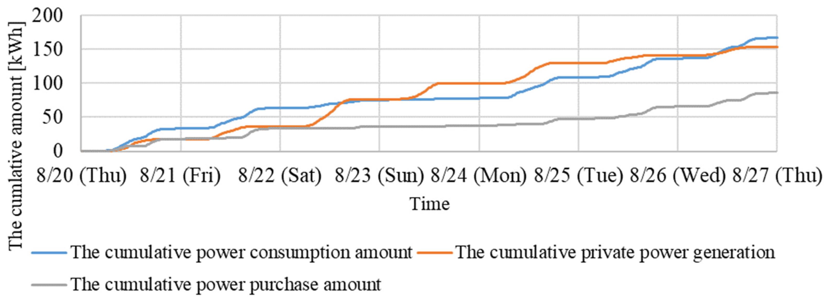
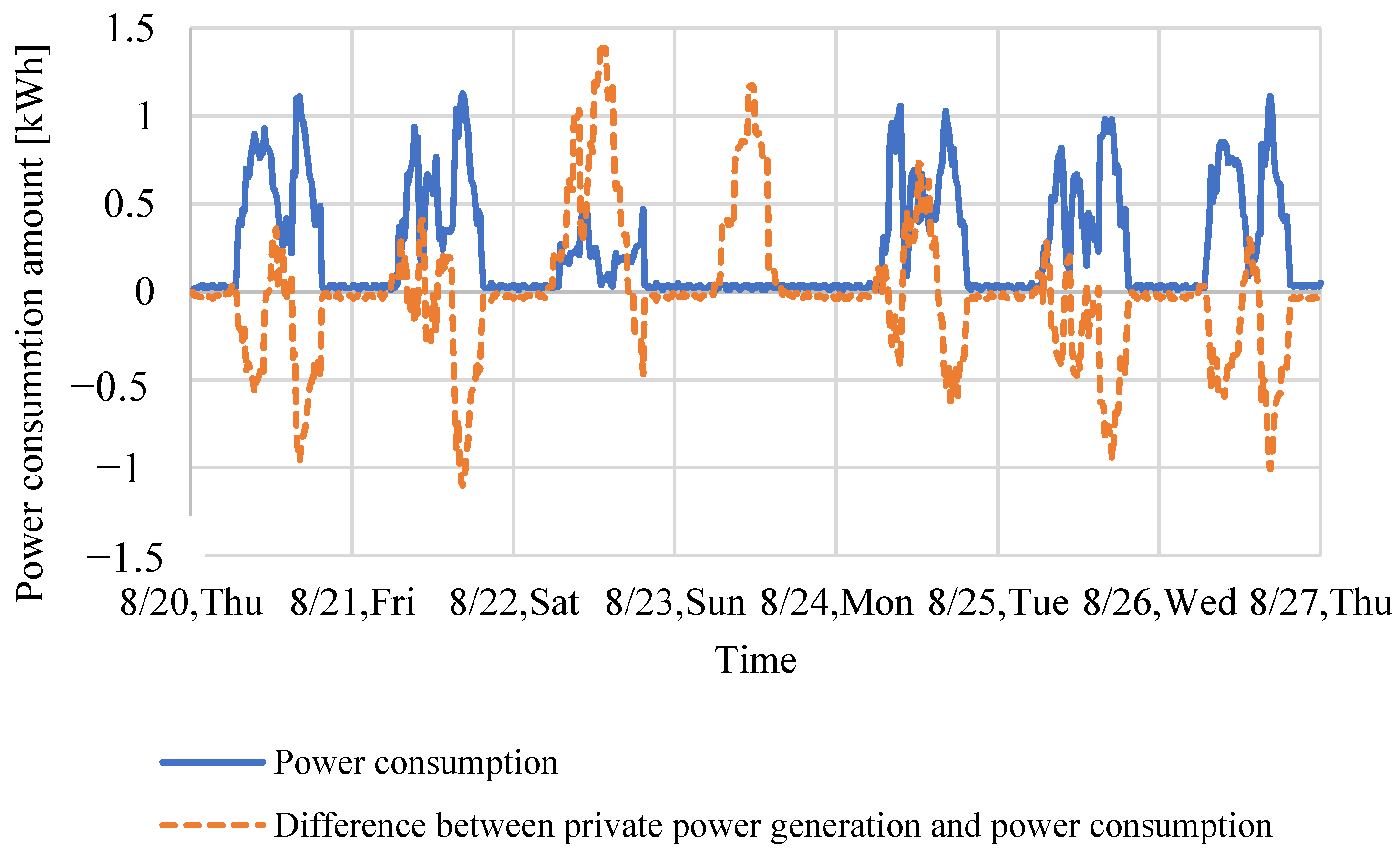
- The difference in the cumulative power consumption and the private power generation amounts during the course of the week analyzed was minimal. Results show that appropriate demand-to-supply management could be employed to cover private consumption with private power generation from PV sources;
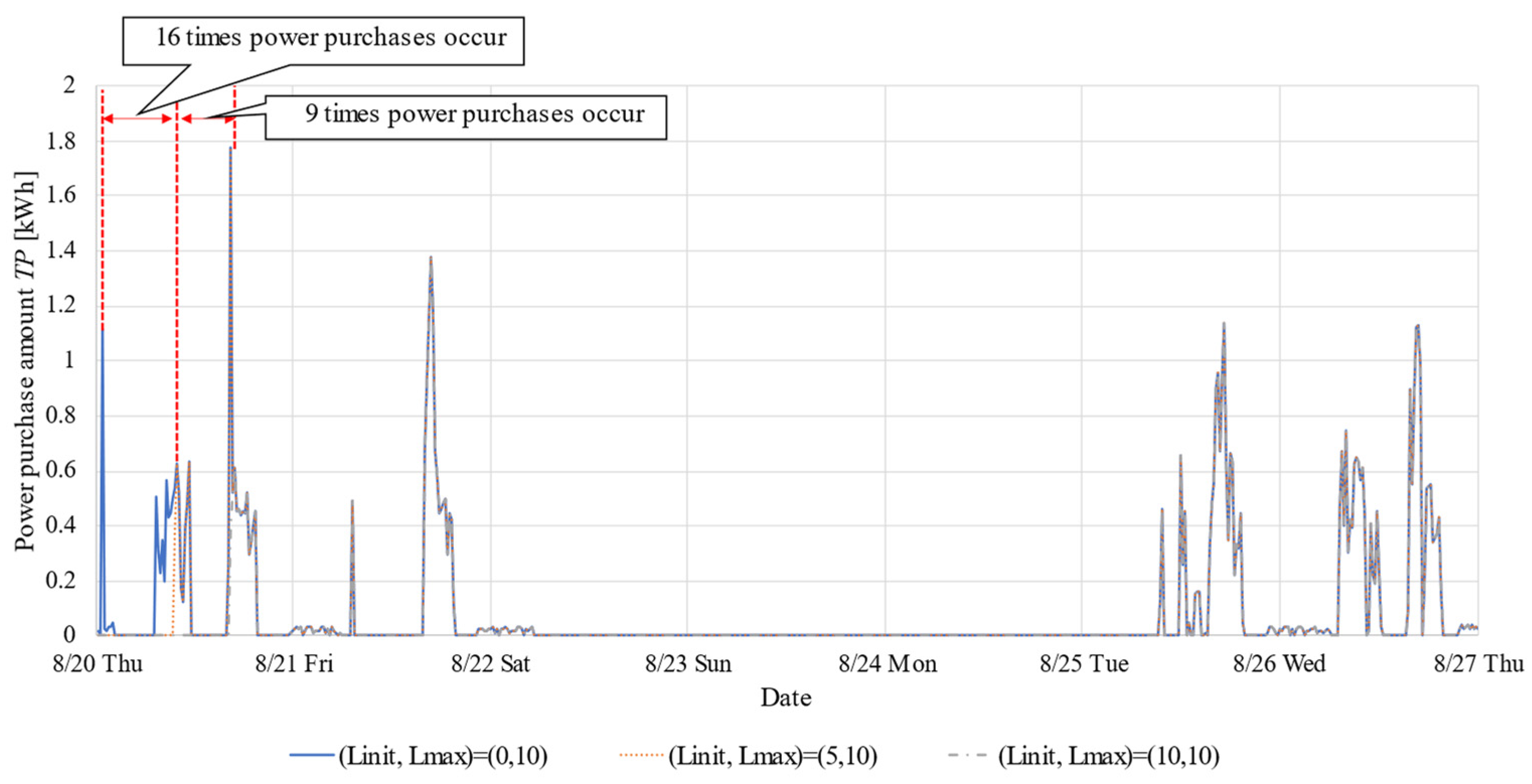
- The cumulative amount of power purchased during this one week, however, corresponded to approximately half of the cumulative power consumption. It was also shown that the total number of power purchases comprised ~70%, indicating that private power generation was not fully utilized;
- Power consumption exceeded that of private power generation during the morning hours of 6:00–12:00, and the afternoon hours around 16:00 for all days except Sunday, when the facility was closed. It was also shown from shifts in the updating of by Matsui logic that these were crucial hours for demand-to-supply management;
- It was shown that in the moving base storage amount obtained from the cumulative probability distribution of the remaining storage amount on a cloudy day, it was difficult to manage days where the daylight hours and total solar radiation were favorable or holidays where power consumption was minimal;
- A sensitivity analysis of the total power purchase amount showed that an effective combination of the initial and the maximum storage amount could be obtained simultaneously through the on-demand DSMM;
- The amount of changes in the total number of power purchases was inconsistent;
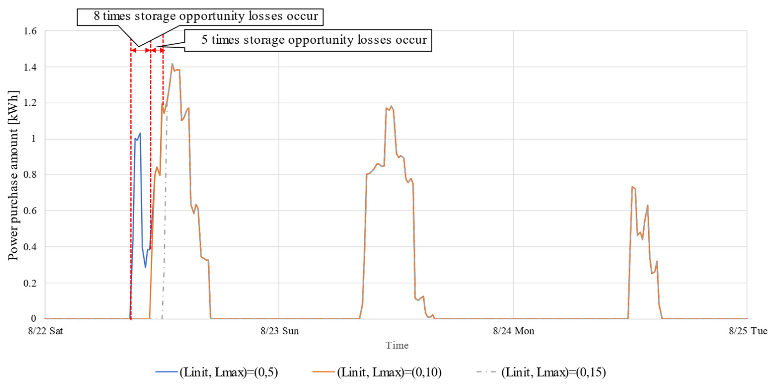
- It was not preferable to have a certain amount of initial inventory when setting the supply–demand management start day as Thursday because the storage opportunity loss would arrive earlier due to a full charge;
- With regard to the storage opportunity loss amount, it was found that the total number of storage opportunity losses did not necessarily correspond to times when there was a change of 5 [kWh];
Author Contributions
Funding
Institutional Review Board Statement
Informed Consent Statement
Data Availability Statement
Acknowledgments
Conflicts of Interest
Appendix A
| Variables | This Study |
|---|---|
| : | Sum of private power generation and purchased electrical power in period t [KWh] |
| : | Sum of the next private power generation and the next power purchase amount in period t [kWh] |
| : | Power consumption amount in period t [kWh] |
| : | Remaining storage capacity in period t [kWh] |
| : | Moving base storage capacity in period t [kWh] |
| : | Forecasted power consumption amount in period t [kWh] |
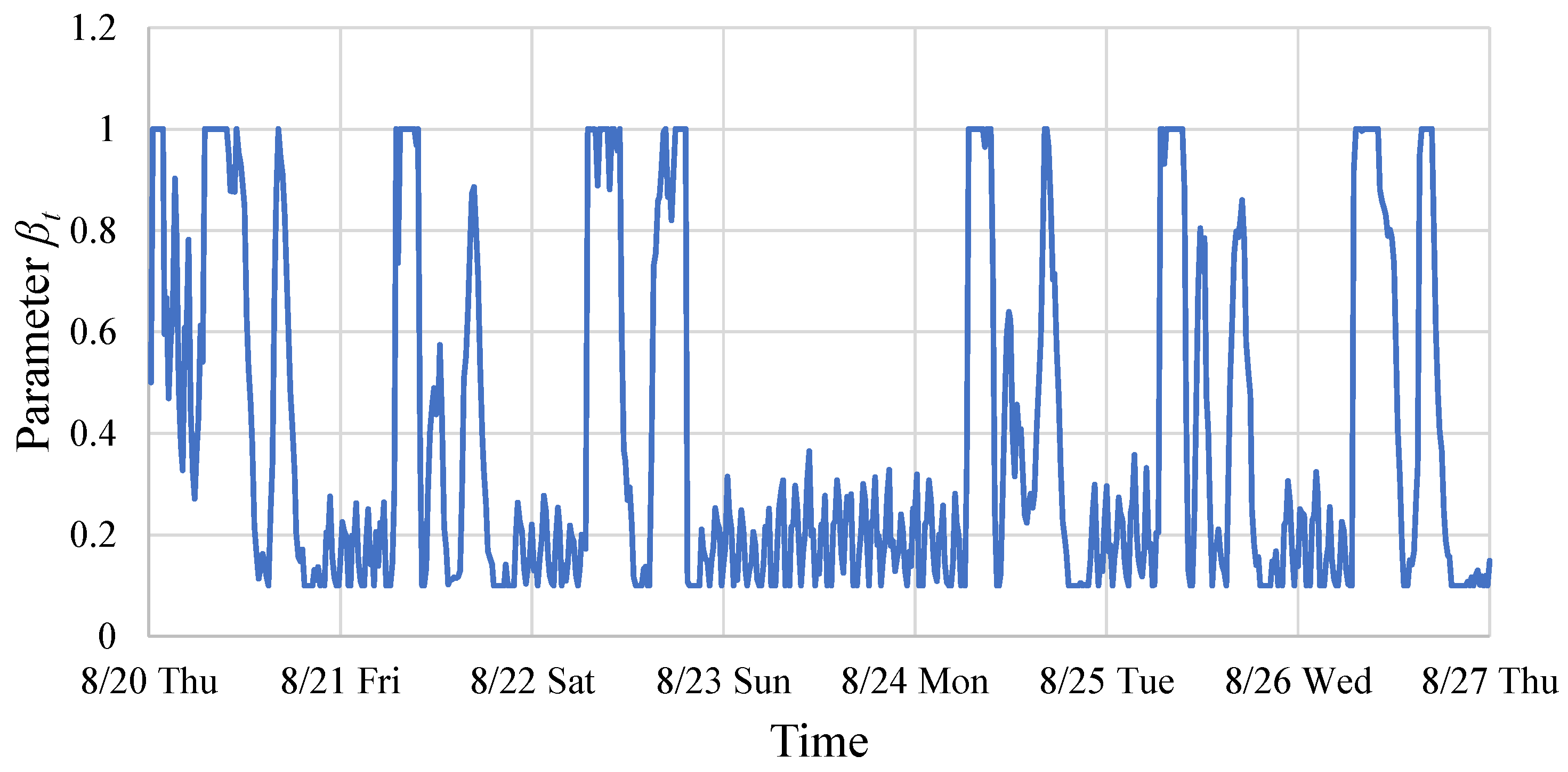
| : | Demand rate at period t |
| : | Input amount determination parameter in period t |
| : | Private power generation in period t [kWh] |
| : | Power purchase amount in period t [kWh] |
| : | Forecasted private power generation in period t [kWh] |
| Coefficient | |
| : | Coefficient of real power consumption |
| : | Cost coefficient for maintaining electricity storage [yen/kWh] |
| : | Cost coefficient for understocked storage [yen/kWh] |
| : | Cost coefficient for overstocked electricity is storage [yen/kWh] |
| Evaluation Value | |
| : | Initial storage capacity [kWh] |
| : | Maximum storage capacity [kWh] |
| : | Storage opportunity loss amount in period t [kWh] |
| : | Total amount of power purchase [kWh] |
| : | Total number of power purchases [number] |
| : | Total number of storage opportunity loss [number] |
| Date | Day and Night | Weather |
|---|---|---|
| 20 August | Day | Rainy, then sometimes cloudy |
| Night | Cloudy, with brief rain | |
| 21 August | Day | Cloudy, then rain for a while |
| Night | Cloudy | |
| 22 August | Day | Cloudy, then sunny |
| Night | Cloudy, sometimes sunny | |
| 23 August | Day | Cloudy, with brief sun |
| Night | Cloudy, with brief sun | |
| 24 August | Day | Cloudy |
| Night | Cloudy | |
| 25 August | Day | Cloudy, then rain for a while |
| Night | Rainy, with brief cloud | |
| 26 August | Day | Rainy |
| Night | Cloudy, sometimes rainy, then sunny for a while | |
| 27 August | Day | Cloudy |
| Night | Cloudy, then rainy for a while |
References
- UNFCCC. The 26th session of the Conference of the Parties to the United Nations Framework Convention on Climate Change, “Glasgow Climate Pact”. Available online: https://unfccc.int/sites/default/files/resource/cop26_auv_2f_cover_decision.pdf (accessed on 9 December 2021).
- BBC News. Biden: This will be ‘Decisive Decade’ for Tackling Climate Change. Available online: https://www.bbc.com/news/science-environment-56837927 (accessed on 31 May 2021).
- Ministry of Economy, Trade and Industry. Government Trends in Green Innovation. Available online: https://www.meti.go.jp/english/press/2020/1111_002.html (accessed on 24 March 2022).
- Ministry of the Environment. Annual Environmental White Paper 2020; Nikkei Printing Inc.: Tokyo, Japan, 2020. (In Japanese)
- Environmental Business Online. Cabinet Decides on Long-Term Strategy Against Global Warming to Realize a Decarbonized Society. Available online: https://www.kankyo-business.jp/column/022598.php (accessed on 24 March 2022).
- Agency for Natural Resources and Energy: What is Renewable Energy? 2020. Available online: https://www.enecho.meti.go.jp/category/saving_and_new/saiene/renewable/outline/index.html (accessed on 21 September 2020).
- Ootake, H. Application of meteorological technology to the field of photovoltaic power generation and energy management. Commun. Oper. Res. Soc. Jpn. 2020, 65, 5–11. (In Japanese) [Google Scholar]
- Agyekum, E.B.; PraveenKumar, S.; Alwan, N.T.; Velkin, V.I.; Shcheklein, S.E. Effect of dual surface cooling of solar photovoltaic panel on the efficiency of the module: Experimental investigation. Heliyon 2021, 7, e07920. [Google Scholar] [CrossRef] [PubMed]
- Agyekum, E.B.; PraveenKumar, S.; Alwan, N.T.; Velkin, V.I.; Shcheklein, S.E.; Yaqoob, S. Experimental investigation of the effect of a combination of active and passive cooling mechanism on the thermal characteristics and efficiency of solar pv module. Inventions 2021, 6, 63. [Google Scholar] [CrossRef]
- Agyekum, E.B.; PraveenKumar, S.; Alwan, N.T.; Velkin, V.I.; Adebayo, T.S. Experimental study on performance enhancement of a photovoltaic module using a combination of phase change material and aluminum fins—Exergy, energy and economic (3e) analysis. Inventions 2021, 6, 69. [Google Scholar] [CrossRef]
- Agyekum, E.B.; PraveenKumar, S.; Eliseev, A.; Velkin, V.I. Design and construction of a novel simple and low-cost test bench point-absorber wave energy converter emulator system. Inventions 2021, 6, 20. [Google Scholar] [CrossRef]
- PraveenKumar, S.; Agyekum, E.B.; Alwan, N.T.; Velkin, V.I.; Yaqoob, S.J.; Adebayo, T.S. Thermal management of solar photovoltaic module to enhance output performance: An experimental passive cooling approach using discontinuous aluminum heat sink. Int. J. Renew. Energy Res. 2021, 11, 1700–1712. [Google Scholar] [CrossRef]
- Matsui, M.; Hujikawa, H.; Ishi, N. Supply Chain Management Towards Post ERP/SCM; Asakura Publishing Co., Ltd.: Tokyo, Japan, 2009. [Google Scholar]
- Matsui, M. Management of Production Companies: Profit Maximization and Factory Science; Asakura Publishing Co., Ltd.: Tokyo, Japan, 2005. [Google Scholar]
- Usuki, J.; Kitaoka, M. Classification of cumulative curve from initial inventory and relationship between inventory quantity and lead time. J. Jpn. Ind. Manag. Assoc. 2001, 51, 558–565. (In Japanese) [Google Scholar] [CrossRef]
- Wichmann, M.G.; Johannes, C.; Spengler, T.S. Energy-oriented Lot-Sizing and Scheduling considering energy storages. Int. J. Prod. Econ. 2019, 216, 204–214. [Google Scholar] [CrossRef]
- Moon, J.; Park, J. Smart production scheduling with time-dependent and machine-dependent electricity cost by considering distributed energy resources and energy storage. Int. J. Prod. Res. 2014, 52, 3922–3939. [Google Scholar] [CrossRef]
- Uhlemair, H.; Karschin, I.; Geldermann, J. Optimizing the production and distribution system of bioenergy villages. Int. J. Prod. Econ. 2014, 147, 62–72. [Google Scholar] [CrossRef]
- Trappey, A.J.C.; Trappey, C.V.; Liu, P.H.Y.; Lin, L.; Ou, J.J.R. A hierarchical cost learning model for developing wind energy infrastructures. Int. J. Prod. Econ. 2013, 146, 386–391. [Google Scholar] [CrossRef]
- Pham, A.; Jin, T.; Novoa, C.; Qin, J. A multi-site production and microgrid planning model for net-zero energy operations. Int. J. Prod. Econ. 2019, 218, 260–274. [Google Scholar] [CrossRef]
- Jahanpour, E.; Ko, H.S.; Nof, S.Y. Collaboration protocols for sustainable wind energy distribution networks. Int. J. Prod. Econ. 2016, 182, 496–507. [Google Scholar] [CrossRef]
- Rentizelas, A.A.; Tolis, A.I.; Tatsiopoulos, I.P. Investment planning in electricity production under CO2 price uncertainty. Int. J. Prod. Econ. 2012, 140, 622–629. [Google Scholar] [CrossRef] [Green Version]
- Xydis, G. A techno-economic and spatial analysis for the optimal planning of wind energy in Kythira island, Greece. Int. J. Prod. Econ. 2013, 146, 440–452. [Google Scholar] [CrossRef] [Green Version]
- Takanokura, M.; Matsui, M.; Tang, H. Energy Management with battery system for smart city. In Proceedings of the 33rd Chinese Control Conference, Nanjing, China, 28–30 July 2014. [Google Scholar]
- Santana-Vieraa, V.; Jimenezb, J.; Jin, T.; Espiritu, J. Implementing factory demand response via onsite renewable energy: A design-of-experiment approach. Int. J. Prod. Res. 2015, 53, 7034–7048. [Google Scholar] [CrossRef]
- Matsui, M.; Uchiyama, H.; Hujikawa, H. Progressive-curve-based control of inventory fluctuation under on-demand SCM. J. Jpn. Ind. Manag. Assoc. 2005, 56, 139–145. (In Japanese) [Google Scholar] [CrossRef]
- Ecolomy Co., Ltd. Website. Available online: https://www.ecolomy.co.jp/ (accessed on 21 September 2020).
- Asada, K.; Iwasaki, T.; Aoyama, Y. An Introduction to Demand Forecasting for Inventory Management; Toyo Keizai Inc.: Tokyo, Japan, 2008. (In Japanese) [Google Scholar]
- Japan Meteorological Agency: Historical Weather Data Search Website. Available online: https://www.data.jma.go.jp/obd/stats/etrn/index.php?prec_no=&block_no=&year=&month=&day=&view=a4 (accessed on 25 November 2020).


| Facility Attributes | Childcare Facility |
|---|---|
| Business hours | 7:00–19:00 on weekdays and Saturdays |
| Data period | 20 August–26 August in a given year |
| Panel power generation output | 10 kW |
Publisher’s Note: MDPI stays neutral with regard to jurisdictional claims in published maps and institutional affiliations. |
© 2022 by the authors. Licensee MDPI, Basel, Switzerland. This article is an open access article distributed under the terms and conditions of the Creative Commons Attribution (CC BY) license (https://creativecommons.org/licenses/by/4.0/).
Share and Cite
Ijuin, H.; Yamada, S.; Yamada, T.; Takanokura, M.; Matsui, M. Solar Energy Demand-to-Supply Management by the On-Demand Cumulative-Control Method: Case of a Childcare Facility in Tokyo. Energies 2022, 15, 4608. https://doi.org/10.3390/en15134608
Ijuin H, Yamada S, Yamada T, Takanokura M, Matsui M. Solar Energy Demand-to-Supply Management by the On-Demand Cumulative-Control Method: Case of a Childcare Facility in Tokyo. Energies. 2022; 15(13):4608. https://doi.org/10.3390/en15134608
Chicago/Turabian StyleIjuin, Hiromasa, Satoshi Yamada, Tetsuo Yamada, Masato Takanokura, and Masayuki Matsui. 2022. "Solar Energy Demand-to-Supply Management by the On-Demand Cumulative-Control Method: Case of a Childcare Facility in Tokyo" Energies 15, no. 13: 4608. https://doi.org/10.3390/en15134608
APA StyleIjuin, H., Yamada, S., Yamada, T., Takanokura, M., & Matsui, M. (2022). Solar Energy Demand-to-Supply Management by the On-Demand Cumulative-Control Method: Case of a Childcare Facility in Tokyo. Energies, 15(13), 4608. https://doi.org/10.3390/en15134608