
Energy-Aware Bag-of-Tasks Scheduling in the Cloud Computing System Using Hybrid Oppositional Differential Evolution-Enabled Whale Optimization Algorithm

 ,
,  ,
,  ,
,
Abstract
:1. Introduction
1.1. Research Motivations
1.2. Research Contributions
- (1)
- A hybrid metaheuristic called h-DEWOA is suggested, which uses the search mechanisms of chaotic map and OBL techniques to generate diverse initial population, and integrates the evolutionary DE method with the basic WOA approach to improve search exploration and convergence rate.
- (2)
- The DE metaheuristic is further augmented with the OBL method to improve convergence rate and solution diversity throughout the h-DEWOA approach.
- (3)
- A fitness-aware tradeoff scheme is integrated in the h-DEWOA approach to provide sufficient tradeoff between exploration and exploitation phases, which further helps to improve the quality of scheduling solutions.
- (4)
- Finally, real-workloads of CEA-Curie and HPC2N supercomputing sites are selected for performance evaluation. Simulation results of the proposed h-DEWOA are compared with WOA-based and other state-of-the-art scheduling approaches using extensive experiments. Results and observations clearly show the supremacy of h-DEWOA over baseline algorithms.
2. Related Works
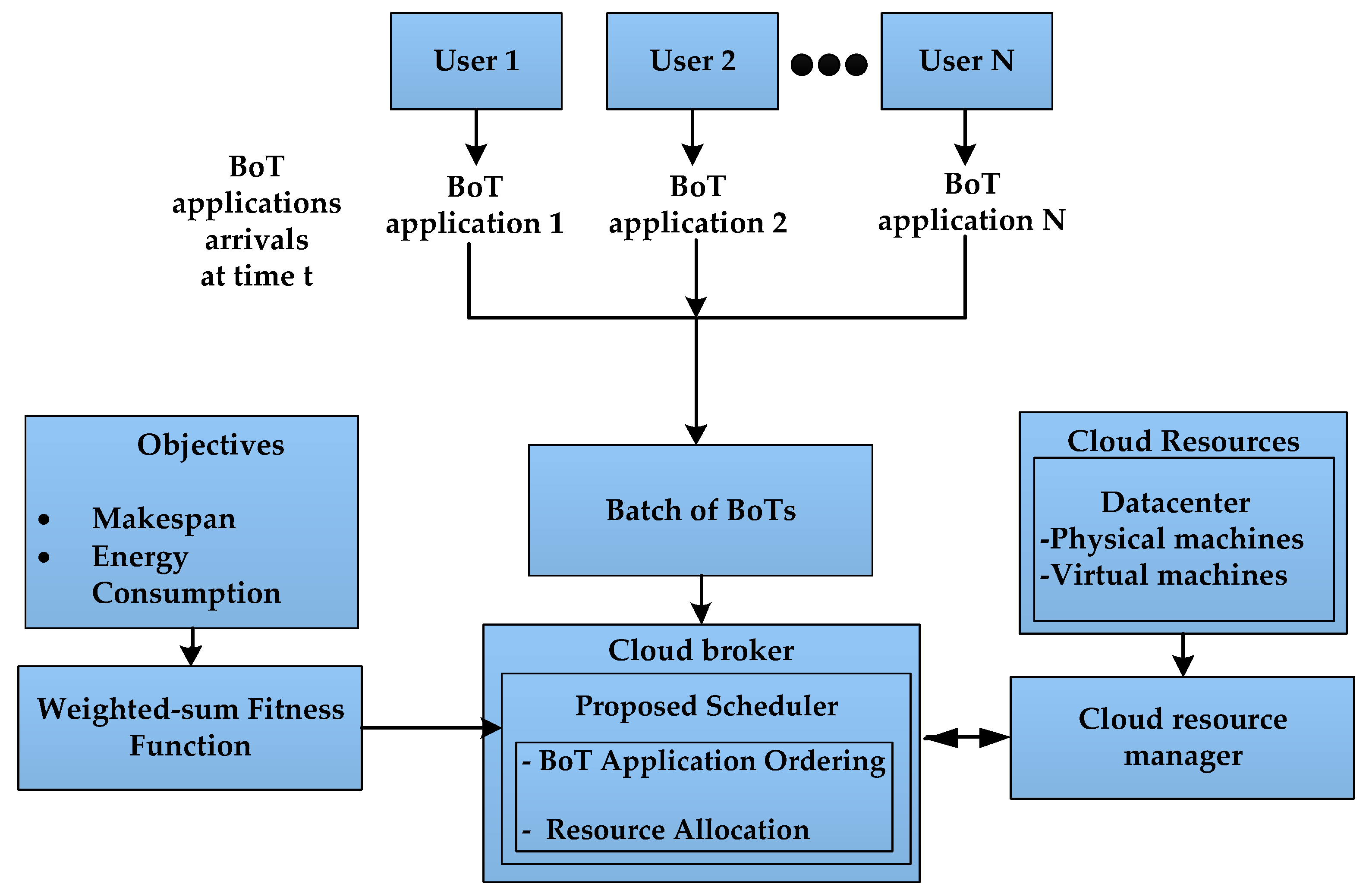
3. System Model and Problem Definition
3.1. Cloud Data Center Model
3.2. BoT Application, Execution Time, and Scheduling Model
3.3. Problem Objectives and Fitness Function
3.3.1. Makespan Model
3.3.2. Energy Model
3.3.3. Fitness Function
- Every BoT application demands a static number of VMs for processing.
- Every VM only processes a single task of the BoT application at a time.
- The numbers of BoT applications and VMs in cloud data center are fixed.
- Deadlines are not associated with the execution of BoT applications.
4. Proposed Scheduling Methodology
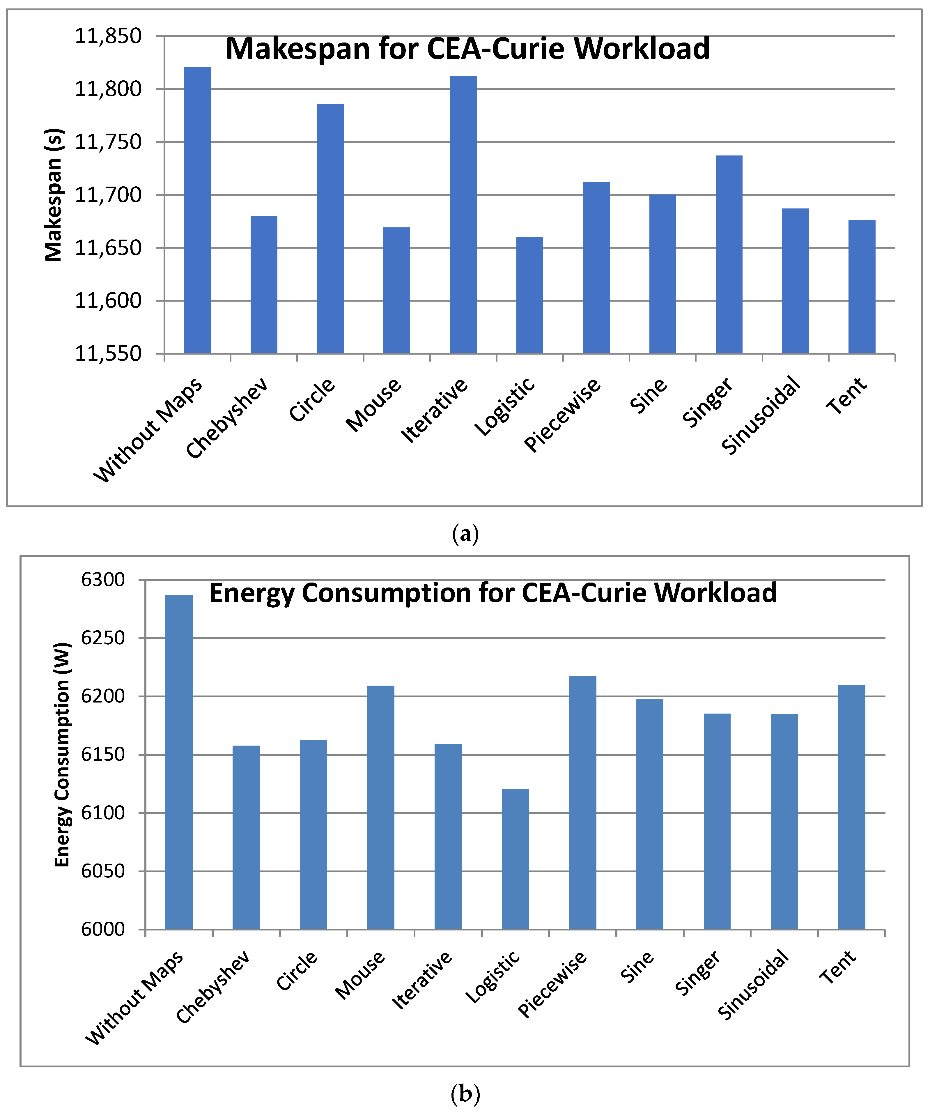
4.1. Chaotic Maps (CM)
4.2. Opposition-Based Learning (OBL)
4.3. Whale Optimization Algorithm (WOA)
4.3.1. Encircling Prey (When |A| < 1 and p < 0.5)
4.3.2. Bubble-Net Attacking (Exploitation Process)
Shrinking Encircling Mechanism
Spiral updating position (When |A| < 1 and p < 0.5)
4.3.3. Search for Prey
4.4. Differential Evolution (DE)
4.4.1. DE Mutation Operator
4.4.2. DE Crossover Operator
4.4.3. DE Selection Operator
4.5. Limitations of the Standard WOA Approach
4.6. Proposed h-DEWOA Algorithm
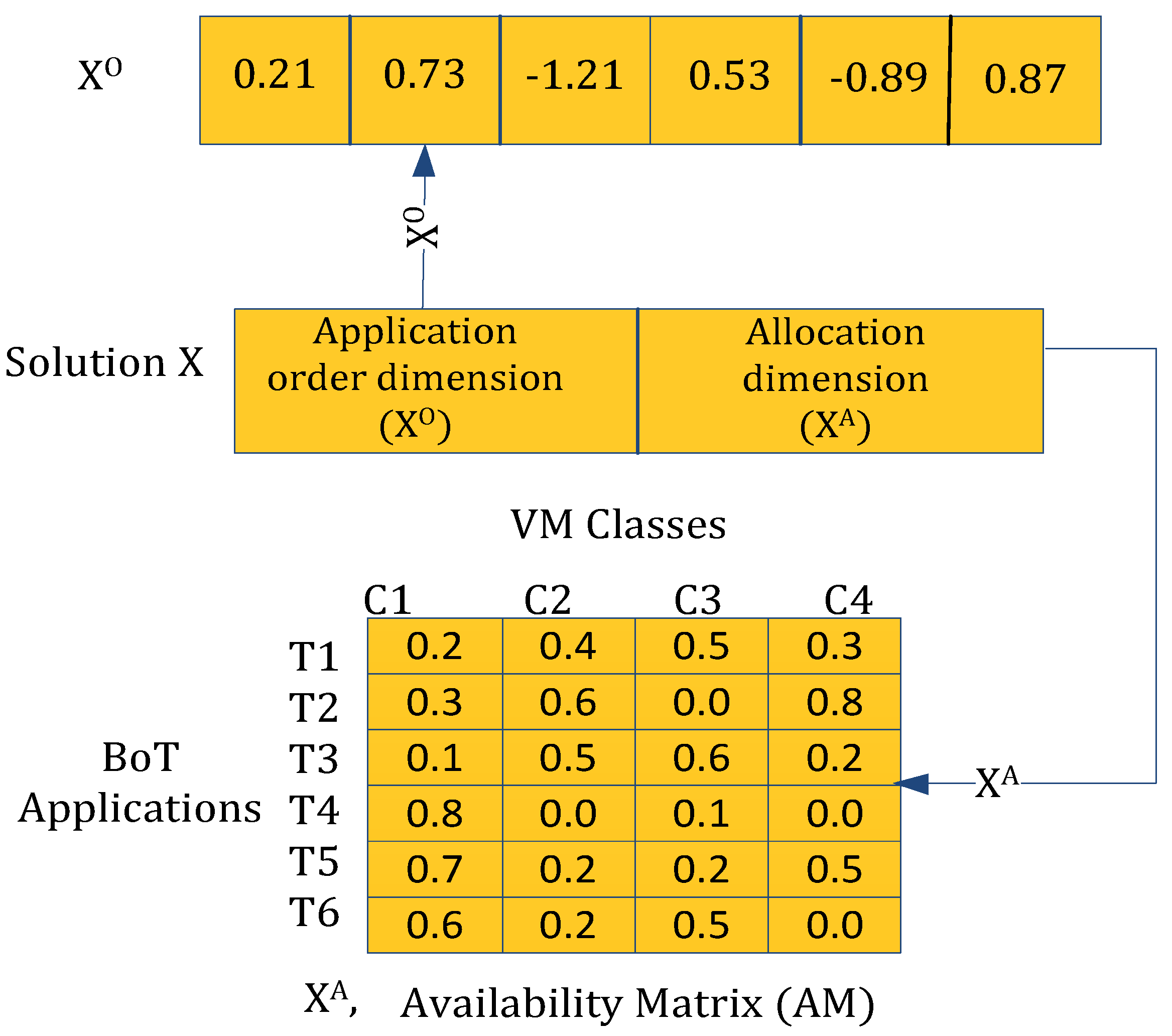
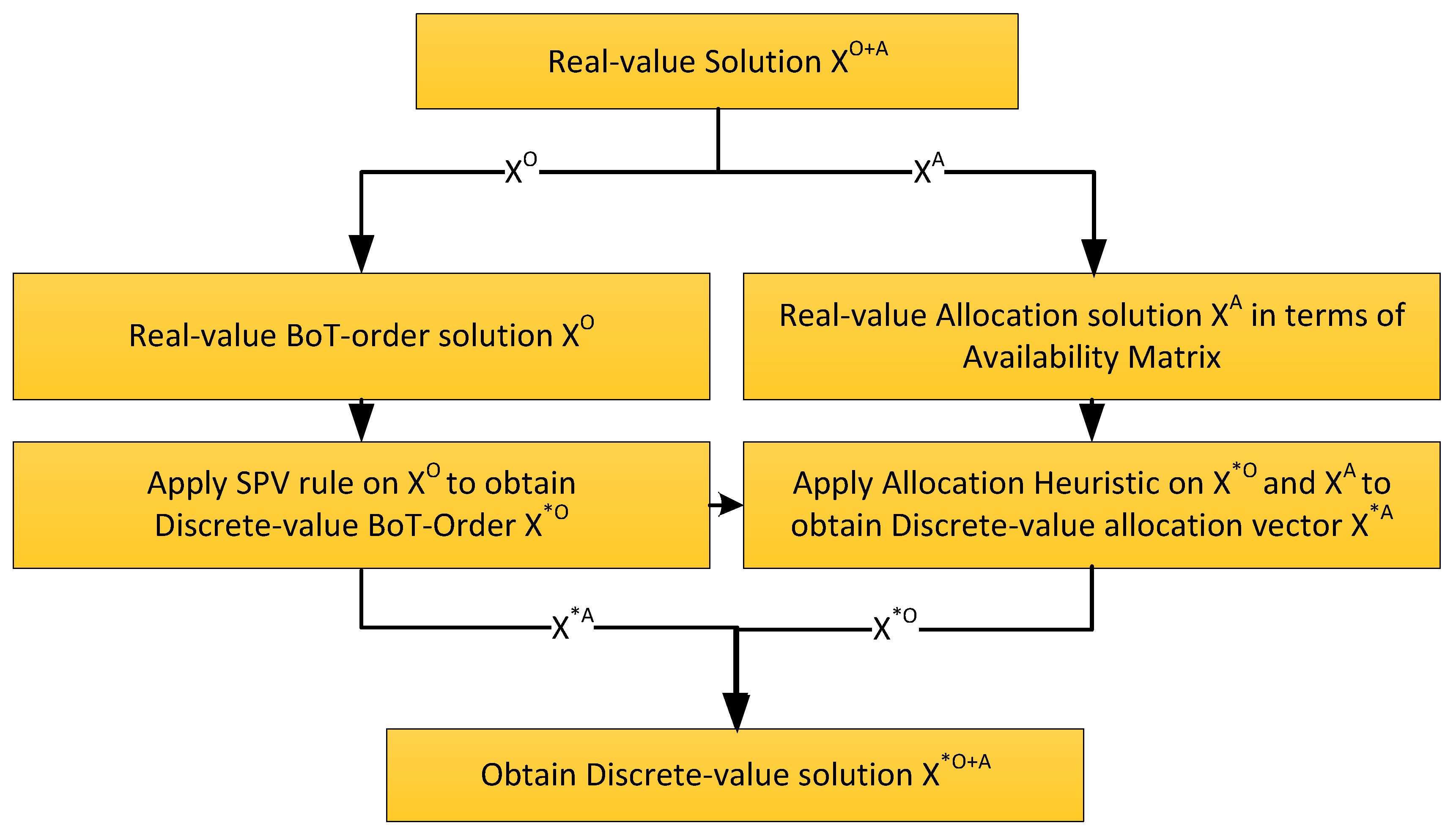
4.6.1. Solution Encoding
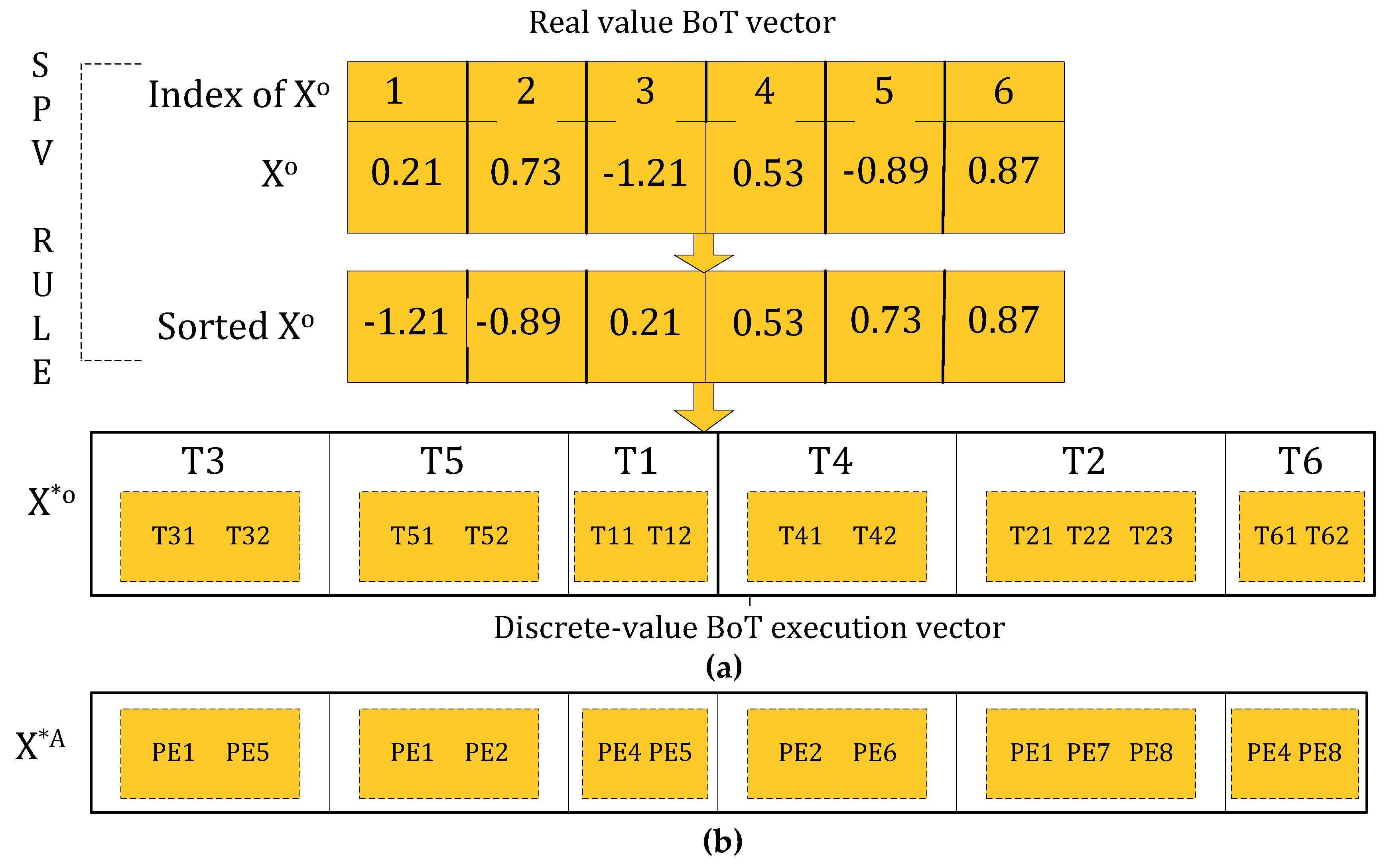
Discretization of BoT Application-Order Vector
| Algorithm 1. SPV method. |
| Input: Real-value BoT application-order vector |
| Output: Discrete BoT application-order vector |
| 1. Begin |
| 2. Sort in the increasing order |
| 3. Calculate with discrete-values where |
| 4. End |
Discretization of Resource Allocation Vector
| Algorithm 2. MDeRA heuristic. |
| Input: PM: Total physical machines (pm), VM: Total virtual machines (vm), |
| vms.PM: Virtual machines (vm) in each pm, CBA: Set of concurrent BoT applications |
| Require: AM matrix representing VMs availability |
| Result: Allocation list (AL): a pair of (BoT application ∈ CBA, vm ∈ VM) |
| 1. Sort available BoTs in CBA in the ascending order of their expected execution time |
| 2. for each BoT application ∈ CBA do |
| 3. Apply DeRA heuristic [13]. |
| 4. end for |
4.6.2. Pseudo-Code of the h-DEWOA Algorithm
| Algorithm 3. h-DEWOA Algorithm. |
| Input: Tasks, Virtual machines, fitness function: ObjFn(X), |
| Variables: PX,G: Real-value population, PXD,G: Equivalent discrete-value population, G: Generation index; N: Population size, Gmax: Total generations |
| Output: *: Best solution containing discrete-value BoT-order and resource allocation |
| 1: Initialization of parameters of scheduling problem, WOA, and DE metaheuristics |
| 2: G = 1//First generation for producing initial population |
| 3: PXChaotic,G ← ½ ChaoticInitialPopulation( )//First half of initial real-value population using logistic map |
| 4: PXOBL,G ← ½ OBLbasedInitialPopulation( )//Second half of initial real-value population using OBL |
| 5: PX,G ← PXChaotic,G + PXOBL,G //Merge both halves of initial real-value population |
| 6: PXD,G←MDeRA(SPV(PX,G)) //Generate discrete-form population using SPV and MDeRA heuristics |
| 7: Fitness (PXD,G) ← ObjFn(PXD,G) //Evaluate the fitness of population |
| 8: * = argmin (Fitness (PXD,G)) //Global best discrete-value solution |
| 9: * ) //Global best real-value solution |
| 10. G = G + 1 |
| 11: while (G < MaxGeneration) |
| 12: for each solution X𝑖,G ∈ population PX,G do |
| 13: if (Fitness (solution X𝑖,G) <= Fitness(gBestG−1)) //Exploration–exploitation tradeoff condition |
| 14: for both task-order and allocation dimensions of solution X𝑖,G do//WOA Exploitation |
| 15: Apply WOA on solution X𝑖,G using Equation (13) and Equation (18) to obtain X𝑖,G+1 |
| 16: Store position if X𝑖,G+1 is better than X𝑖,G |
| 17: end for //WOA phase ends |
| 18: else (Fitness (solution X𝑖,G) > Fitness(gBestG−1)) |
| 19: for both task-order and allocation dimensions of solution X𝑖,G do//DE Exploration |
| 20: Generate Mutant of X𝑖,G using Equation (22) |
| 21: Crossover of Mutant with the original solution using Equation (23) |
| 22: Obtain solution X𝑖,G+1 using selection operator using Equation (24) |
| 23: Apply OBL on X𝑖,G+1//Apply OBL on DE solution to improve exploration |
| 24: Retain best solution among OBL- and non-OBL-based DE solution |
| 25: end for //DE phase ends |
| 26: end if |
| 27: end for |
| 28: PXD,G← MDeRA(SPV(PX,G))//Generate discrete-form population |
| 29: Fitness (PXD,G) ← ObjFn(PXD,G) //Fitness evaluation Evaluate the fitness of population |
| 30: Update the current integer and real-value global best solution |
| 31: end while |
| 32: * = argmin (Fitness (PXD,G))//Record the global best scheduling solution found |
- Line 1: Initialize parameters of the scheduling problem, WOA algorithm, and DE algorithm
- Line 2: Initialize G equal to 1
- Line 3: Generate first random half of initial real-value population using logistic chaotic maps.
- Line 4: Generate second random half of initial real-value population using opposition-based learning method.
- Line 5: Merge both initial population halves generated in Line 2 and 3 to generate full initial real-value population.
- Line 6: Convert real-form population into an equivalent discrete-form population using SPV and MDeRA heuristic.
- Line 7: Evaluate the fitness of the population using objective function.
- Line 8: Find the global best discrete-value solution from whole population
- Line 9: Generate the real-value population
- Line 10: Update G value
- Line 11: Iterations of the h-DEWOA using while loop till (G < MaxGeneration) condition is true
- Line 12: Start of the for loop to update the position of solutions
- Line 13–17: Exploration–exploitation tradeoff condition is tested on the basis of fitness of current solution (Line 13). When the current solution’s fitness is equal to or better than the previous generation population’s global best solution (Line 13), then WOA exploitation mechanism is applied on the current solution position to search nearby better solutions (Line 14–17).
- Line 18–25: When the current solution’s fitness is less than the previous generation population’s global best solution (Line 18), the h-DEWOA algorithm performs DE exploration activity for searching better far-away solutions (Line 19–22). After that, OBL is applied on the real-value solution and select the best solution between the OBL solution and non-OBL solution (Line 23–25).
- Line 26: End of if condition for switching between exploration and exploitation.
- Line 27: End of for loop for updating solution position.
- Line 28: Obtain the discrete-form population by applying SPV and MDeRA heuristic.
- Line 29: Evaluate the fitness of new population using fitness function.
- Line 30: This step results in updating of the current integer and real-value global best solution.
- Line 31: End of while loop since algorithm iteration condition is met.
- Line 32: Output the best solution found with minimum fitness, which represents the optimal schedule consisting of BoT application-order and allocation of VMs to BoT applications.
- Initially, both logistic map and OBL are incorporated to produce an optimal initial population, leading to improved exploration and convergence rate thereafter in the later stages of the proposed h-DEWOA approach.
- Thereafter, the DE metaheuristic is added to the traditional WOA to boost the exploration ability and convergence rate. The OBL method is also incorporated in the DE to further maintain population diversity throughout consecutive generations, producing efficient final solutions and improving convergence rate further.
- Further, a fitness-based exploration–exploitation tradeoff mechanism is incorporated in the proposed h-DEWOA method to adequately balance the DE exploration and WOA exploitation phases, which leads to generation of better schedules.
4.7. Time Complexity Analysis
5. Experimentation and Results
5.1. Workloads and Cloud Configuration
5.2. Comparative Results
5.2.1. Comparison with WOA Variants—First Series of Experiments
5.2.2. Baseline WOA Variants
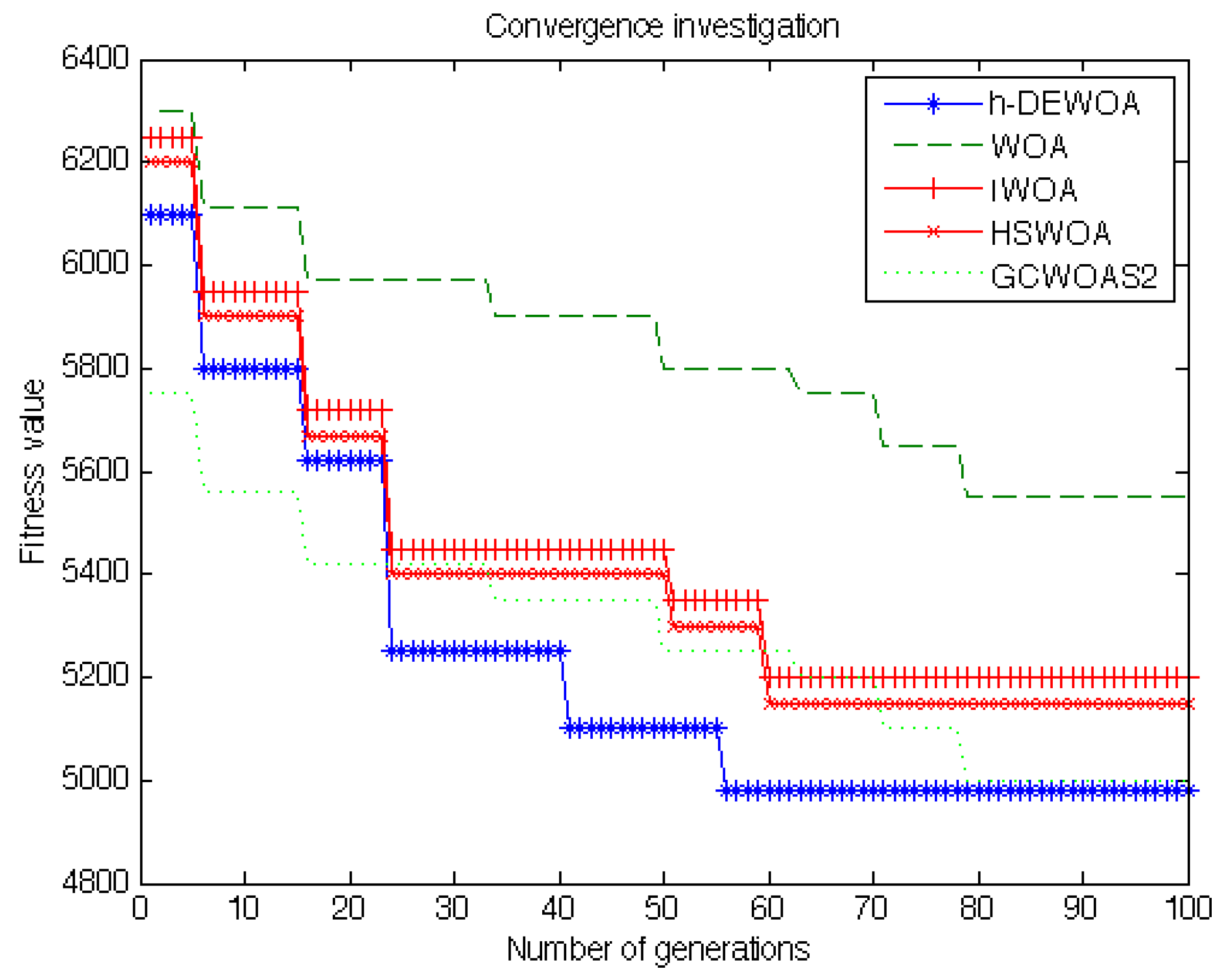
5.2.3. Convergence Examination and Final Values of Parameters
5.2.4. Performance Evaluation of First Set of Experiments
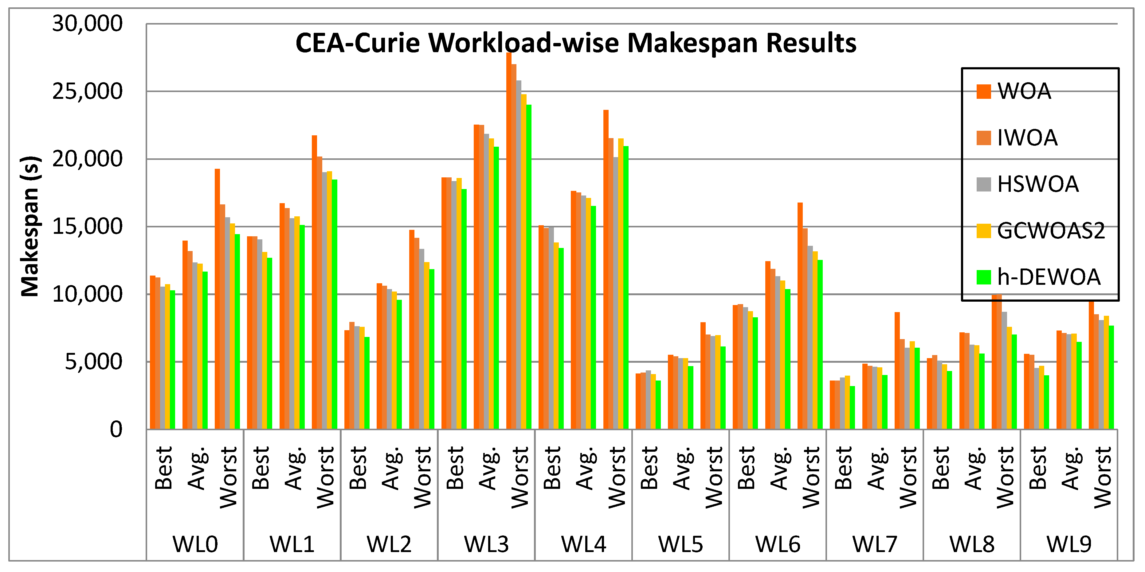
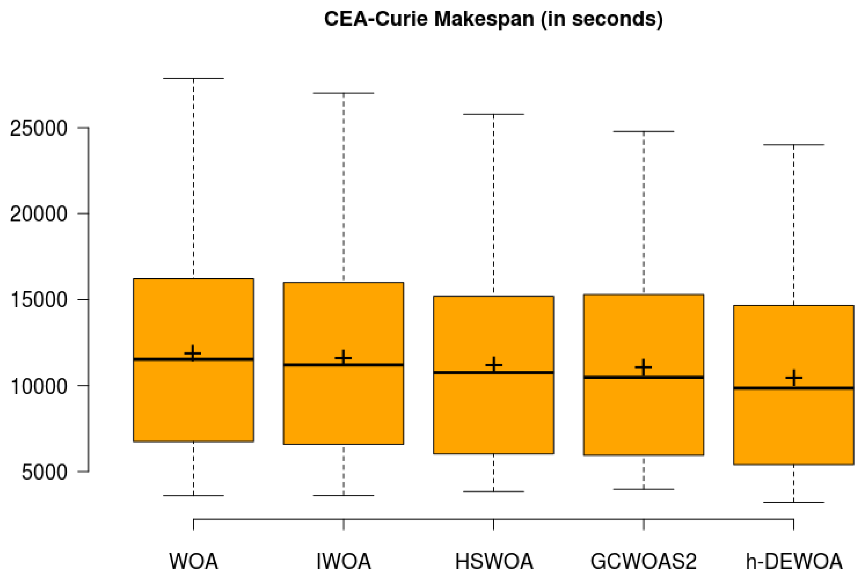
Workload-Wise Makespan Results for CEA-Curie Workloads
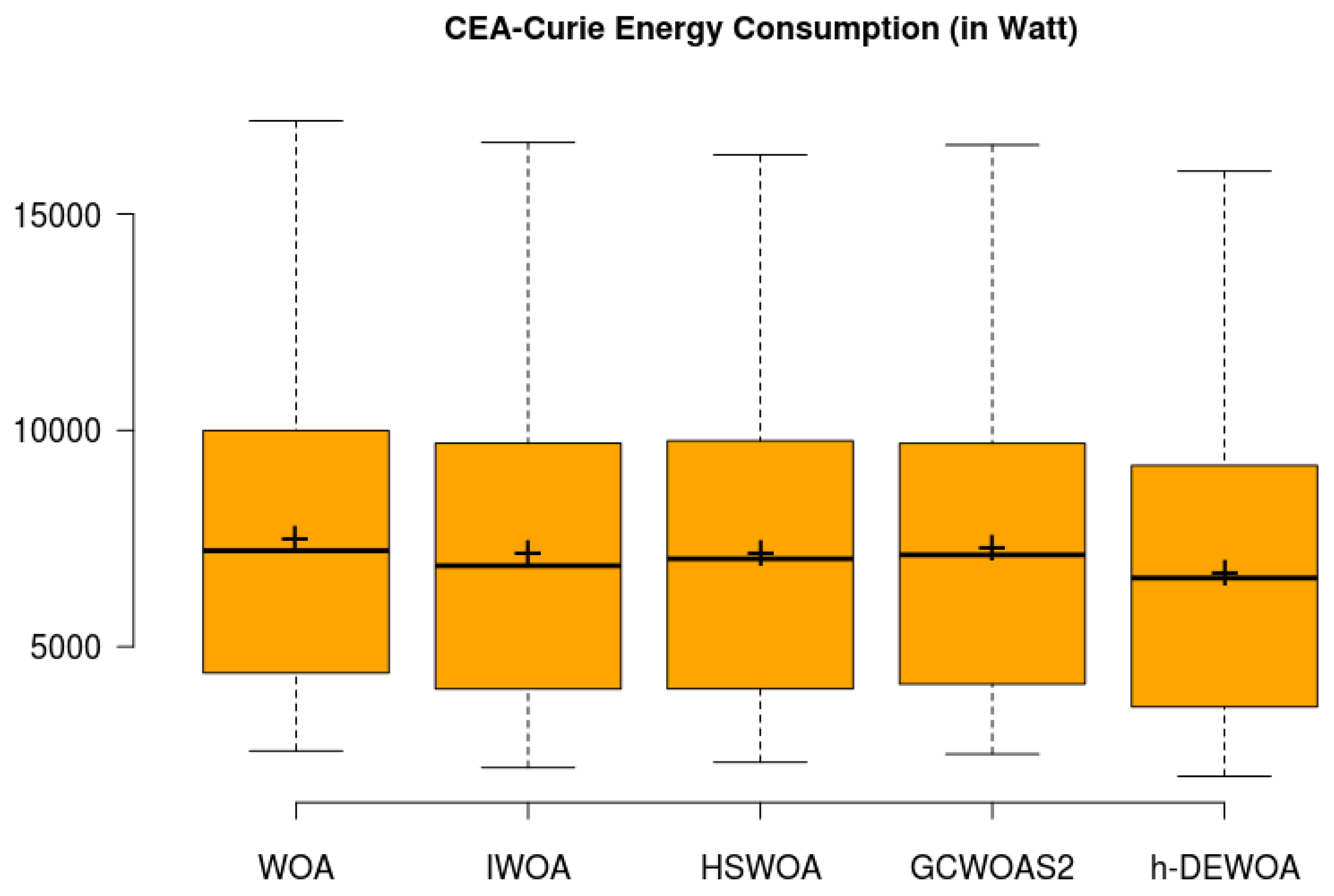
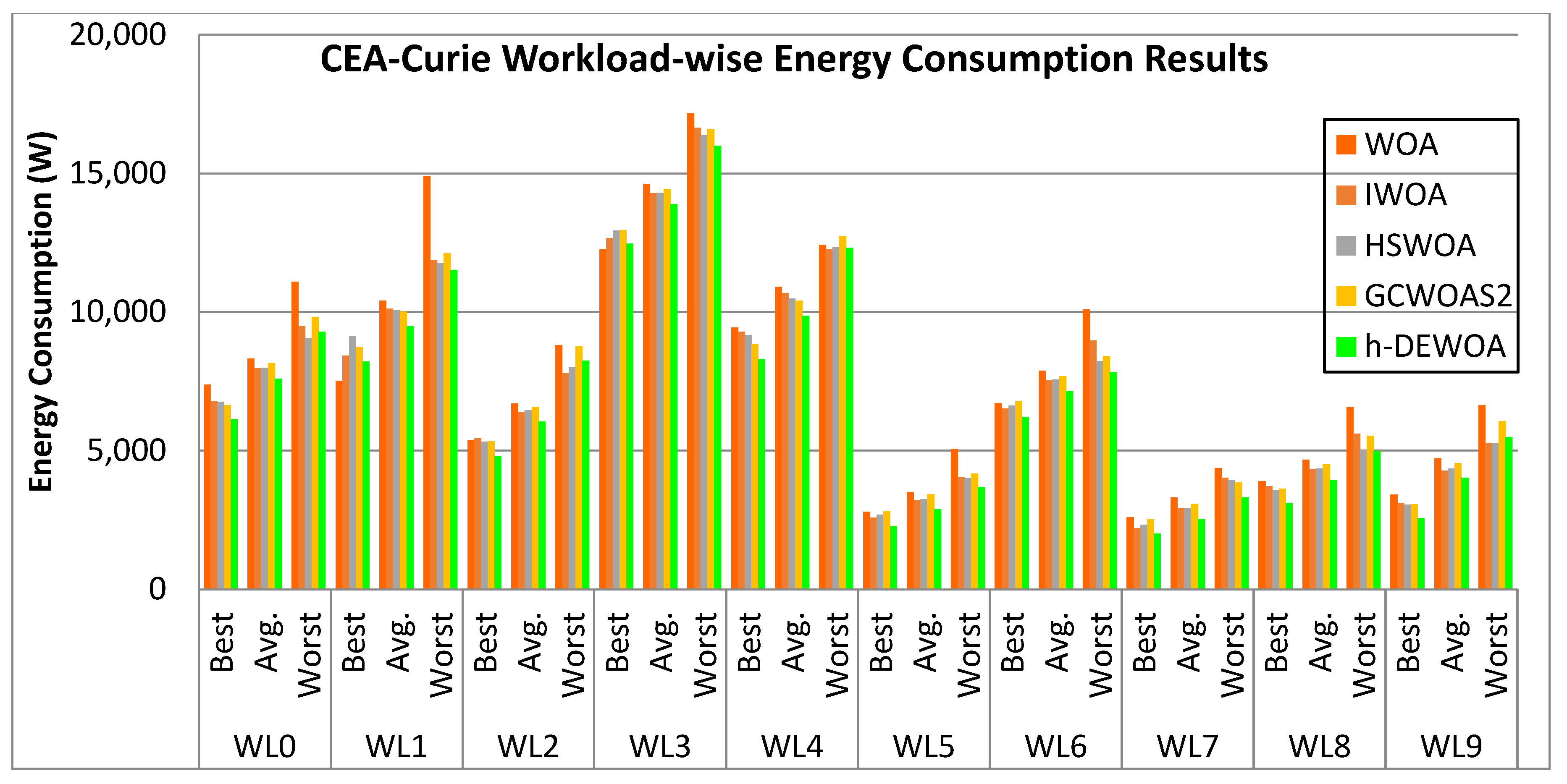
Workload-Wise Energy Consumption Results for CEA-Curie Workloads
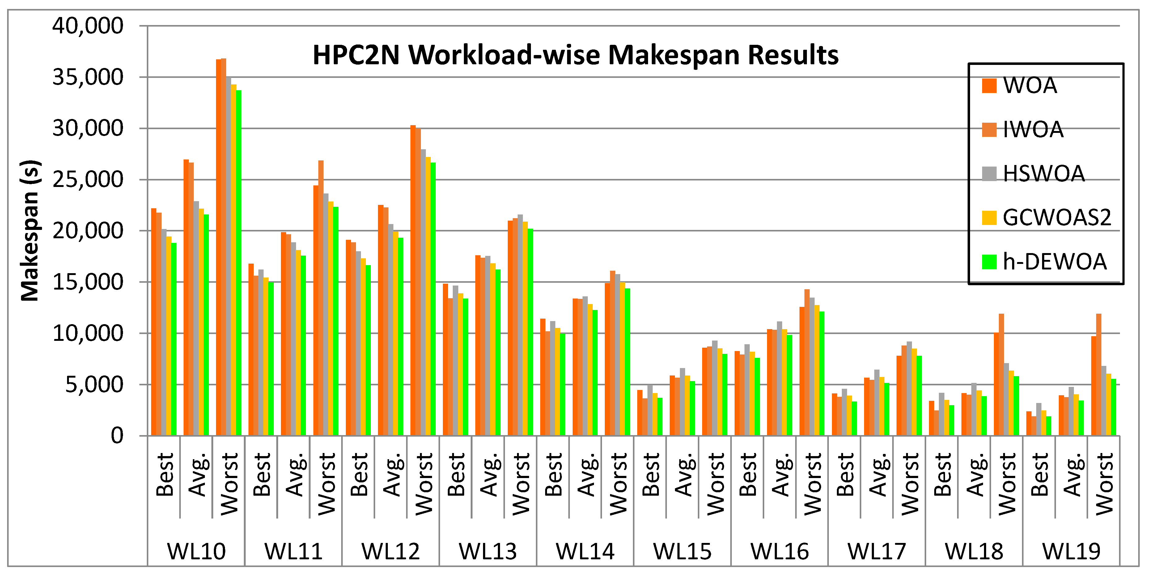
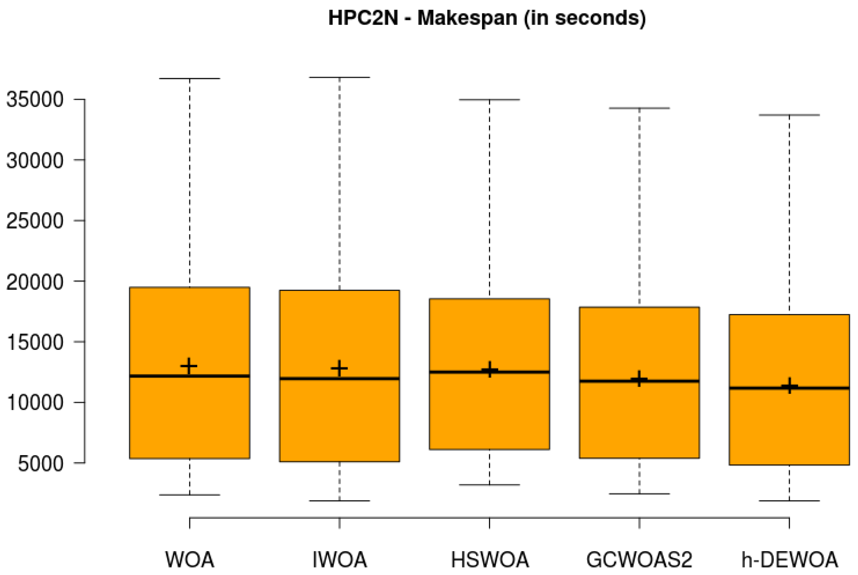
Workload-Wise Makespan Results for HPC2N Workloads
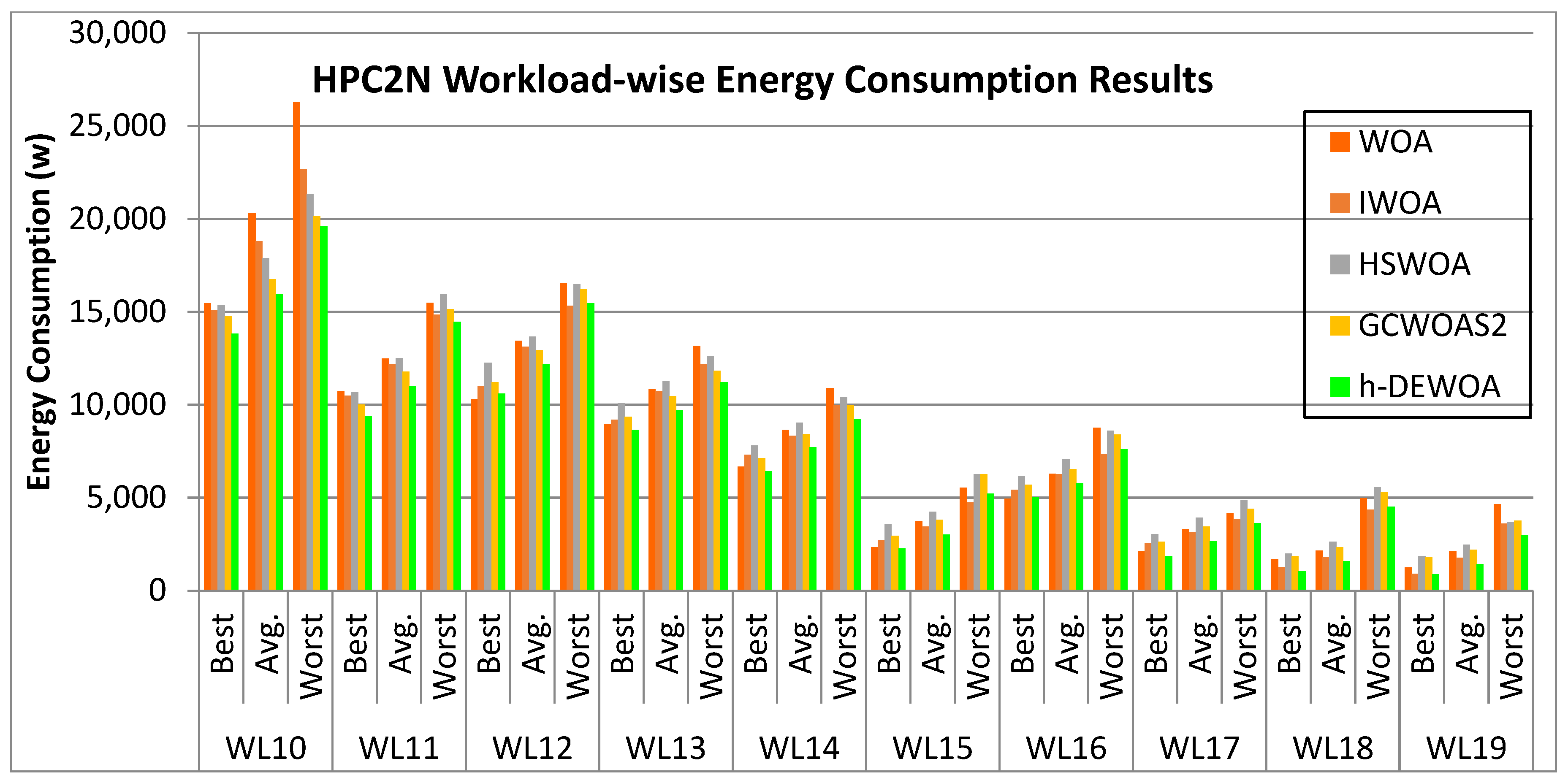
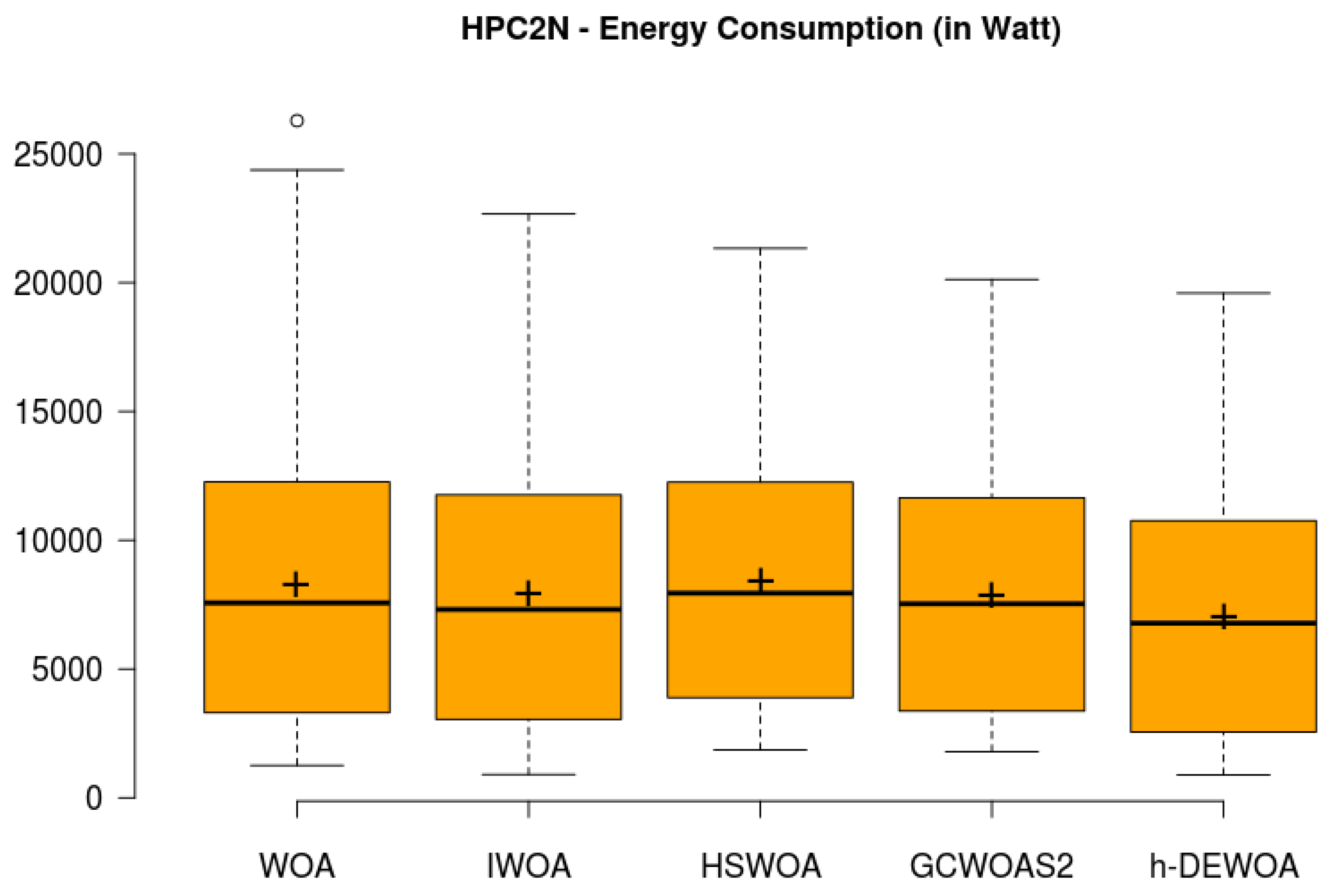
Workload-Wise Energy Consumption Results for HPC2N Workloads
5.2.5. Overall Collective Results—First Set of Experiments
Summarizing the Overall Results—First Series of Experiments
5.3. Comparative Results with State-of-the-Art Algorithms—Second Series of Experiments
5.3.1. Baseline State-of-the-Art Scheduling Algorithms
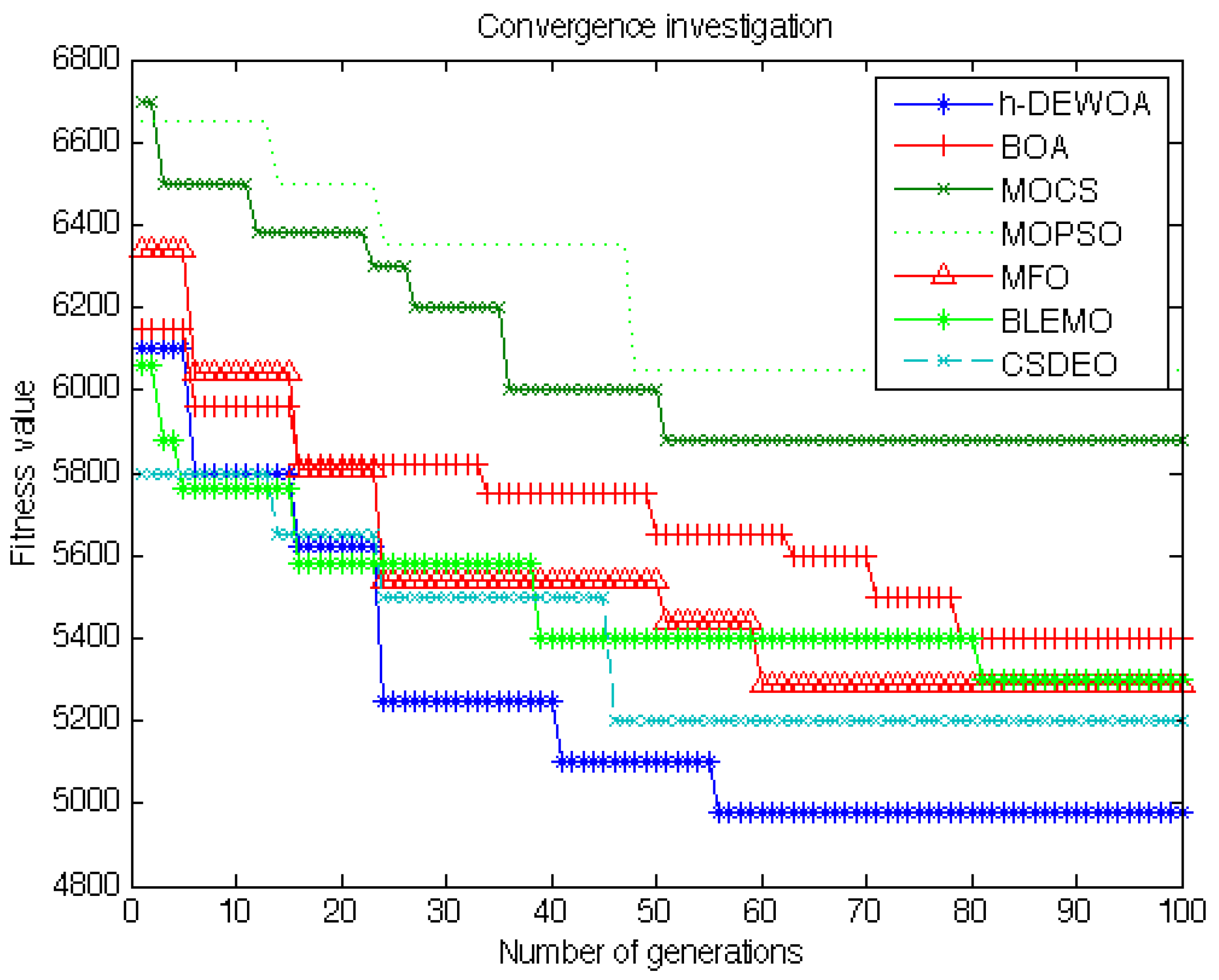
5.3.2. Convergence Examination and Final Values of Parameters
5.3.3. Performance Evaluation of Second Set of Experiments
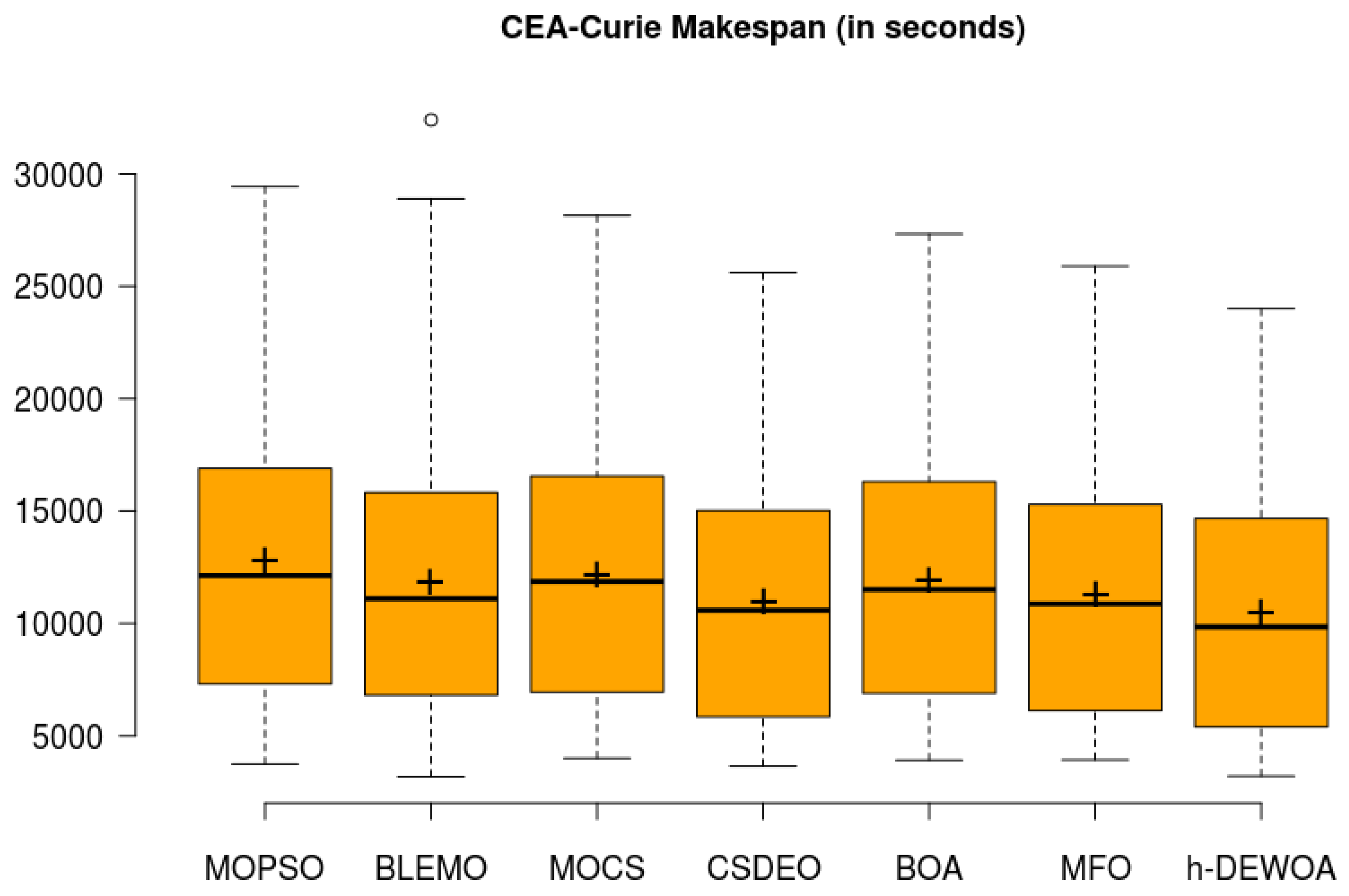
Workload-Wise Makespan Results for CEA-Curie Workloads
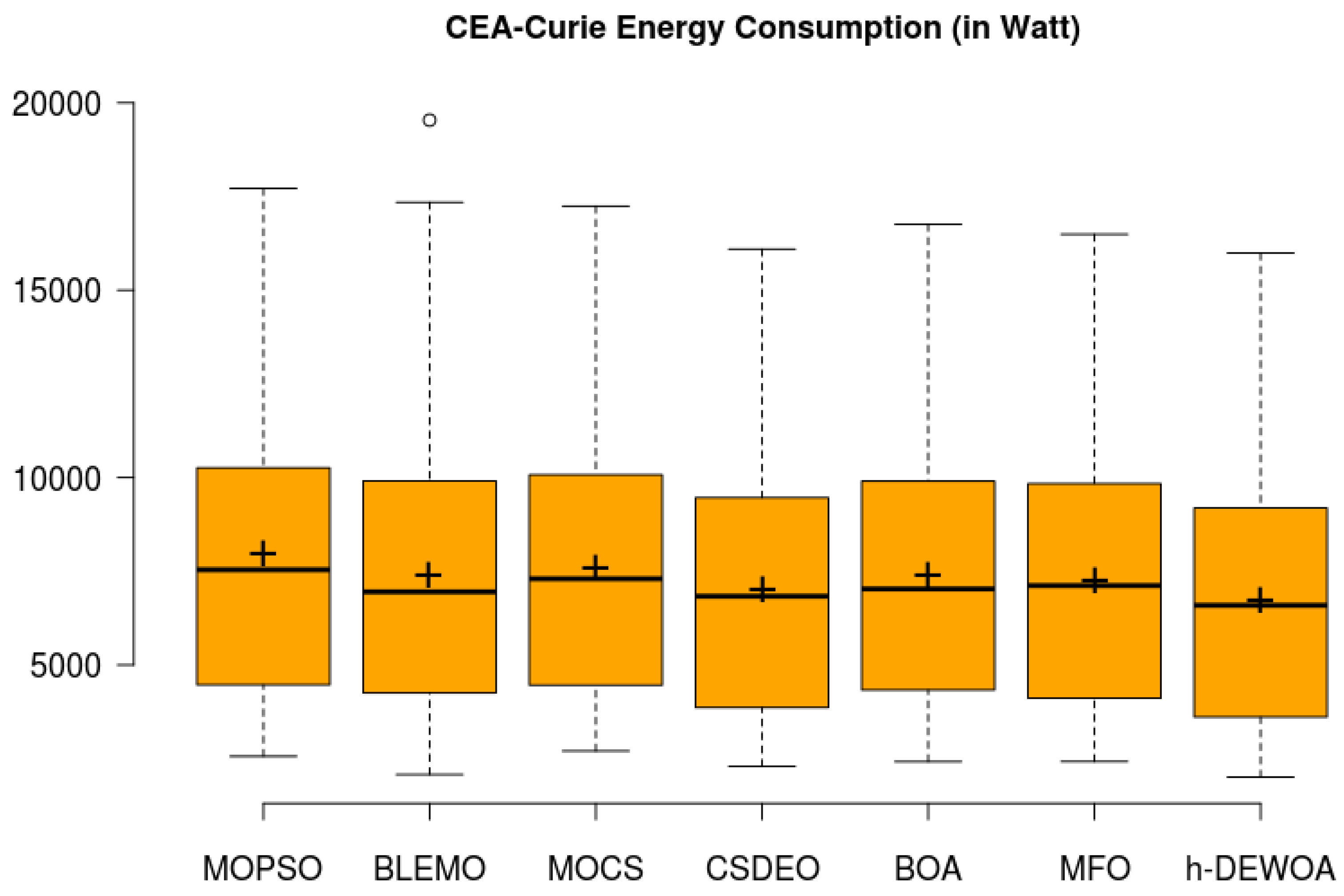
Workload-Wise Energy Consumption Results for WL0–WL9 Workloads
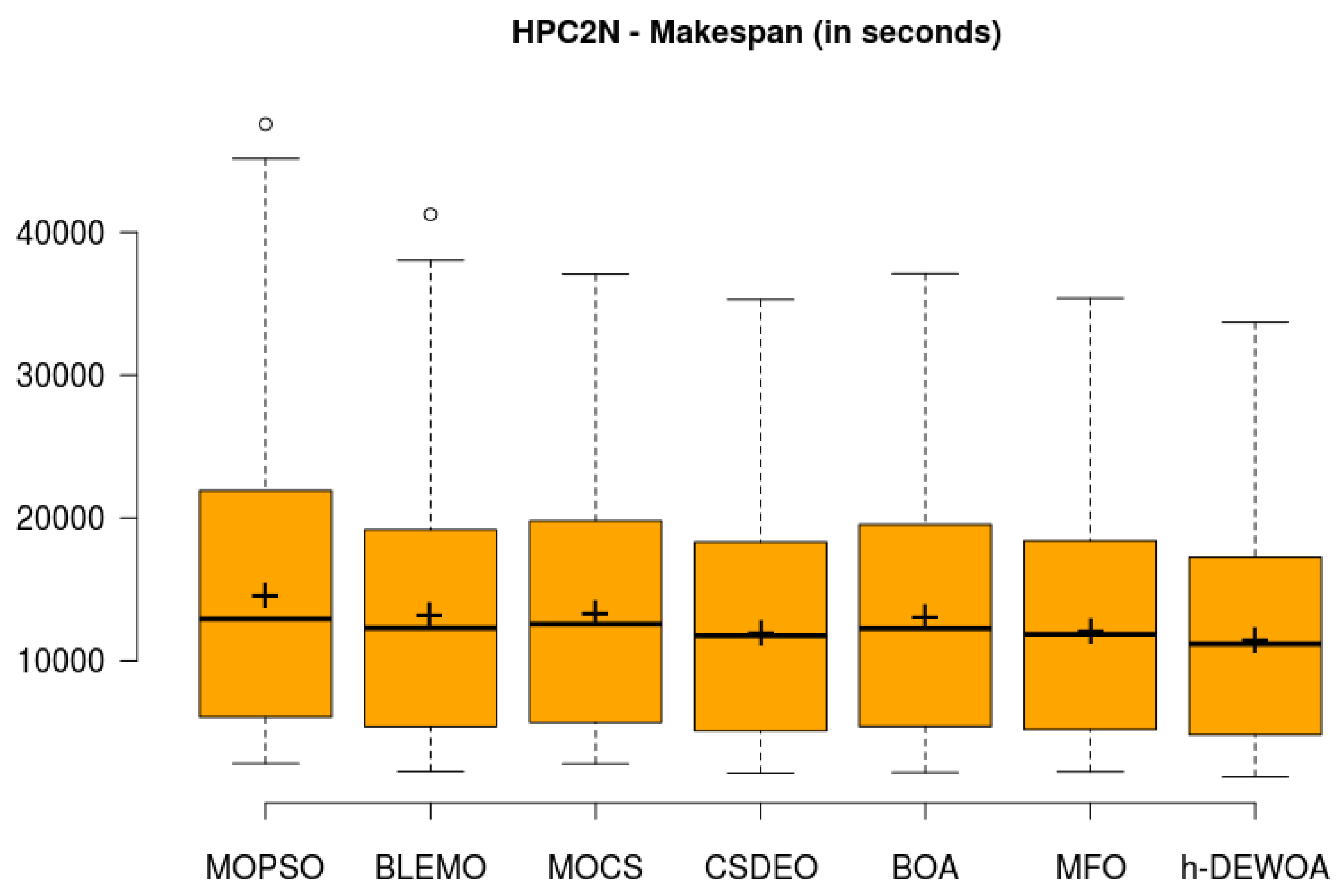
Workload-Wise Makespan Results for HPC2N Workloads
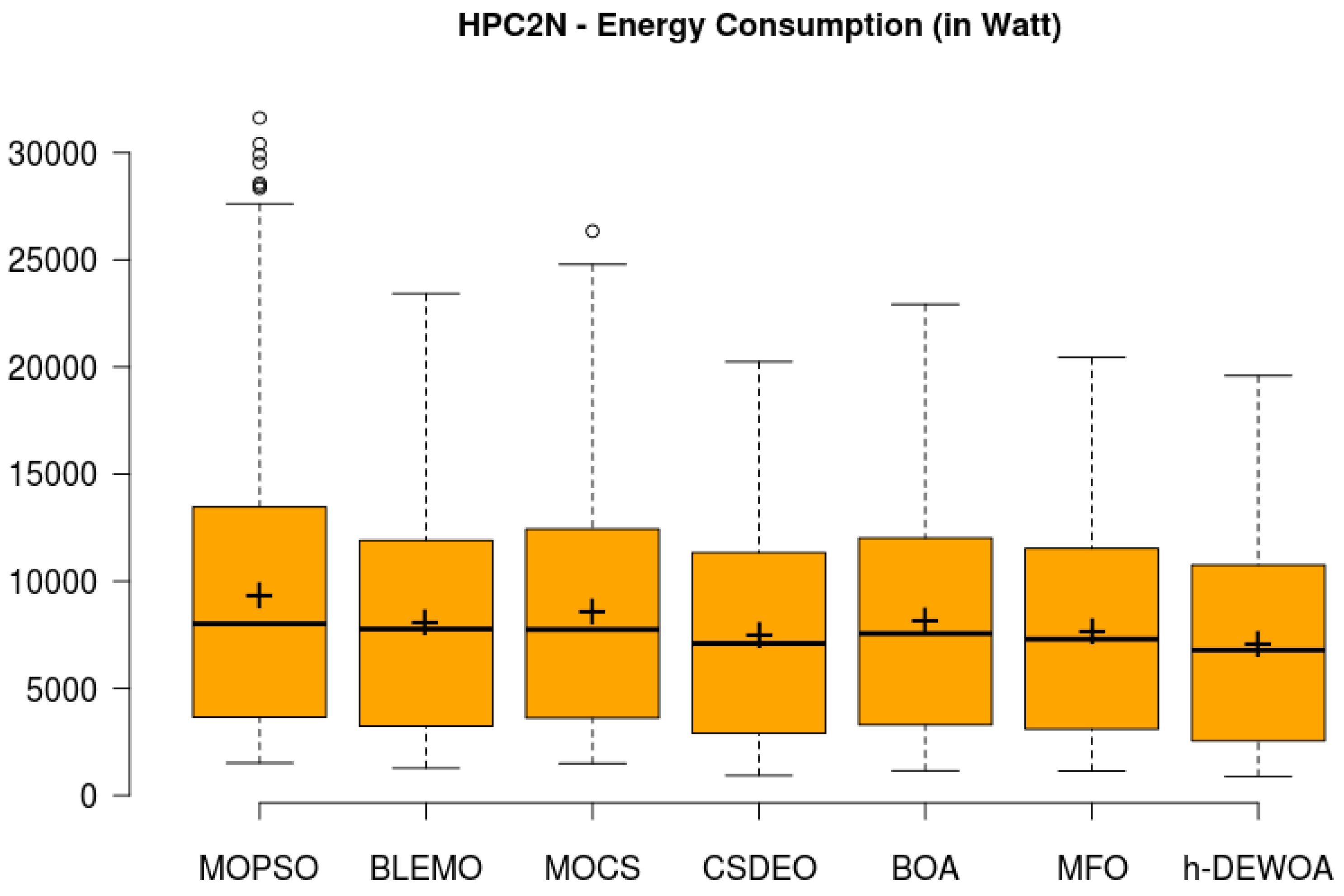
Workload-Wise Energy Consumption Results for HPC2N Workloads
5.3.4. Overall Collective Results—Second Series of Experiments
Summarizing the Overall Results—Second Series of Experiments
5.4. Main Reasons for Excellent Performance of h-DEWOA
6. Conclusions
Author Contributions
Funding
Institutional Review Board Statement
Informed Consent Statement
Data Availability Statement
Acknowledgments
Conflicts of Interest
References
- Moghaddam, S.K.; Buyya, R.; Ramamohanarao, K. Performance-Aware Management of Cloud Resources: A Taxonomy and Future Directions. ACM Comput. Surv. 2019, 52, 1–37. [Google Scholar] [CrossRef] [Green Version]
- Netto, M.A.S.; Calheiros, R.N.; Rodrigues, E.R.; Cunha, R.L.F.; Buyya, R. HPC Cloud for Scientific and Business Applications: Taxonomy, Vision, and Research Challenges. ACM Comput. Surv. 2018, 51, 1–29. [Google Scholar] [CrossRef] [Green Version]
- Amazon EC2 Instance Types-Amazon Web Services. 2022. Available online: https://aws.amazon.com/ec2/instance-types/ (accessed on 6 March 2022).
- Ilager, S.; Ramamohanarao, K.; Buyya, R. ETAS: Energy and thermal-aware dynamic virtual machine consolidation in cloud data center with proactive hotspot mitigation. Concurr. Computat. Pract. Exper. 2019, 31, e5221. [Google Scholar] [CrossRef]
- Khattar, N.; Sidhu, J.; Singh, J. Toward energy-efficient cloud computing: A survey of dynamic power management and heuristics-based optimization techniques. J. Supercomput. 2019, 75, 4750–4810. [Google Scholar] [CrossRef]
- Materwala, H.; Ismail, L. Performance and energy-aware bi-objective tasks scheduling for cloud data centers. Procedia Comput. Sci. 2022, 197, 238–246. [Google Scholar] [CrossRef]
- Brochard, L.; Kamath, V.; Corbalán, J.; Holland, S.; Mittelbach, W.; Ott, M. Energy-Efficient Computing and Data Centers; Wiley: Hoboken, NJ, USA, 2019. [Google Scholar]
- Chhabra, A.; Huang, K.-C.; Bacanin, N.; Rashid, T.A. Optimizing Bag-of-Tasks scheduling on cloud data centers using hybrid swarm-intelligence meta-heuristic. J. Supercomput. 2022, 78, 9121–9183. [Google Scholar] [CrossRef]
- Wolpert, D.H.; Macready, W.G. No free lunch theorems for optimization. IEEE Trans. Evol. Computat. 1997, 1, 67–82. [Google Scholar] [CrossRef] [Green Version]
- Mohamed, A.W.; Hadi, A.A.; Mohamed, A.K. Gaining-sharing knowledge based algorithm for solving optimization problems: A novel nature-inspired algorithm. Int. J. Mach. Learn. Cyber. 2019, 11, 1501–1529. [Google Scholar] [CrossRef]
- Madni, S.H.H.; Abd Latiff, M.S.; Abdullahi, M.; Abdulhamid, S.M.; Usman, M.J. Performance comparison of heuristic algorithms for task scheduling in IaaS cloud computing environment. PLoS ONE 2017, 12, e0176321. [Google Scholar] [CrossRef] [Green Version]
- Sukhoroslov, O.; Nazarenko, A.; Aleksandrov, R. An experimental study of scheduling algorithms for many-task applications. J. Supercomput. 2019, 75, 7857–7871. [Google Scholar] [CrossRef]
- Chhabra, A.; Singh, G.; Kahlon, K.S. Multi-criteria HPC task scheduling on IaaS cloud infrastructures using meta-heuristics. Clust. Comput. 2021, 24, 885–918. [Google Scholar] [CrossRef]
- Kumar, M.; Sharma, S.C.; Goel, A.; Singh, S.P. A comprehensive survey for scheduling techniques in cloud computing. J. Netw. Comput. Appl. 2019, 143, 1–33. [Google Scholar] [CrossRef]
- Amini Motlagh, A.; Movaghar, A.; Rahmani, A.M. Task scheduling mechanisms in cloud computing: A systematic review. Int J. Commun. Syst. 2020, 33, e4302. [Google Scholar] [CrossRef]
- Mostafa Bozorgi, S.; Yazdani, S. IWOA: An improved whale optimization algorithm for optimization problems. J. Comput. Des. Eng. 2019, 6, 243–259. [Google Scholar] [CrossRef]
- Abdel-Basset, M.; Abdle-Fatah, L.; Sangaiah, A.K. An improved Lévy based whale optimization algorithm for bandwidth-efficient virtual machine placement in cloud computing environment. Clust. Comput. 2019, 22, 8319–8334. [Google Scholar] [CrossRef]
- Luan, F.; Cai, Z.; Wu, S.; Jiang, T.; Li, F.; Yang, J. Improved Whale Algorithm for Solving the Flexible Job Shop Scheduling Problem. Mathematics 2019, 7, 384. [Google Scholar] [CrossRef] [Green Version]
- Kaur, G.; Arora, S. Chaotic whale optimization algorithm. J. Comput. Des. Eng. 2018, 5, 275–284. [Google Scholar] [CrossRef]
- Mohammed, H.M.; Umar, S.U.; Rashid, T.A. A Systematic and Meta-Analysis Survey of Whale Optimization Algorithm. Comput. Intell. Neurosci. 2019, 2019, 8718571. [Google Scholar] [CrossRef] [Green Version]
- Lee, K.-C.; Lu, P.-T. Application of Whale Optimization Algorithm to Inverse Scattering of an Imperfect Conductor with Corners. Int. J. Antennas Propag. 2020, 2020, 8205797. [Google Scholar] [CrossRef] [Green Version]
- Ni, L.; Sun, X.; Li, X.; Zhang, J. GCWOAS2: Multiobjective task scheduling strategy based on gaussian cloud-whale optimization in cloud computing. Comput. Intell. Neurosci. 2021, 2021, 5546758. [Google Scholar] [CrossRef]
- Movahedi, Z.; Defude, B.; Mohammad, H.A. An efficient population-based multi-objective task scheduling approach in fog computing systems. J. Cloud Comput. 2021, 10, 53. [Google Scholar] [CrossRef]
- Manikandan, N.; Gopalakrishnan, N.; Pradeep, K. Bee optimization based random double adaptive whale optimization model for task scheduling in cloud computing environment. Comput. Commun. 2022, 187, 35–44. [Google Scholar] [CrossRef]
- Chen, X.; Cheng, L.; Liu, C.; Liu, Q.; Liu, J.; Mao, Y.; Murphy, J. A WOA-based optimization approach for task scheduling in cloud computing systems. IEEE Syst. J. 2020, 14, 3117–3128. [Google Scholar] [CrossRef]
- Jia, L.; Li, K.; Shi, X. Cloud computing task scheduling model based on improved whale optimization algorithm. Wirel. Commun. Mob. Comput. 2021, 2021, 4888154. [Google Scholar] [CrossRef]
- Bezdan, T.; Zivkovic, M.; Bacanin, N.; Strumberger, I.; Tuba, E.; Tuba, M. Multi-objective task scheduling in cloud computing environment by hybridized bat algorithm. IFS 2021, 42, 411–423. [Google Scholar] [CrossRef]
- Muhammad, A.; Abdullah, S.; Samsiah Sani, N. Optimization of Sentiment Analysis Using Teaching-Learning Based Algorithm. Comput. Mater. Contin. 2021, 69, 1783–1799. [Google Scholar] [CrossRef]
- Aldulaimi, M.H.; Zainudin, S.; Bakar, A.A. An improved method to enhance protein structural class prediction using their secondary structure sequences and genetic algorithm. Int. J. Bioinform. Res. Appl. 2018, 14, 376–400. [Google Scholar] [CrossRef]
- Shreem, S.S.; Ahmad Nazri, M.Z.; Abdullah, S.; Sani, N.S. Hybrid Symmetrical Uncertainty and Reference Set Harmony Search Algorithm for Gene Selection Problem. Mathematics 2022, 10, 374. [Google Scholar] [CrossRef]
- Buang, N.; Hanawi, S.A.; Mohamed, H.; Jenal, R. B-Spline Curve Modelling Based on Nature Inspired Algorithms. APJITM 2016, 5. [Google Scholar] [CrossRef]
- Alathamneh, G.M.; Abdullah, S.; Sani, N.S. Genetic Algorithm Selection Strategies based Rough Set for Attribute Reduction. IJCSNS 2019, 19, 187–194. [Google Scholar]
- Albert, P.; Nanjappan, M. WHOA: Hybrid based task scheduling in cloud computing environment. Wirel. Pers. Commun. 2021, 121, 2327–2345. [Google Scholar] [CrossRef]
- Sharma, M.; Garg, R. Energy-aware whale-optimized task scheduler in cloud computing. In Proceedings of the 2017 International Conference on Intelligent Sustainable Systems (ICISS), Palladam, India, 7–8 December 2017; pp. 121–126. [Google Scholar]
- Sreenu, K.; Sreelatha, M. W-Scheduler: Whale optimization for task scheduling in cloud computing. Cluster Comput. 2019, 22, 1087–1098. [Google Scholar] [CrossRef]
- Rekha, P.M.; Dakshayini, M. Efficient task allocation approach using genetic algorithm for cloud environment. Cluster Comput. 2019, 22, 1241–1251. [Google Scholar] [CrossRef]
- Sun, Y.; Li, J.; Fu, X.; Wang, H.; Li, H. Application research based on improved genetic algorithm in cloud task scheduling. J. Intell. Fuzzy Syst. 2020, 38, 239–246. [Google Scholar] [CrossRef]
- Vila, S.; Guirado, F.; Lerida, J.L.; Cores, F. Energy-saving scheduling on IaaS HPC cloud environments based on a multi-objective genetic algorithm. J. Supercomput. 2019, 75, 1483–1495. [Google Scholar] [CrossRef]
- Abdullahi, M.; Ngadi, M.A.; Abdulhamid, S.M. Symbiotic Organism Search optimization based task scheduling in cloud computing environment. Future Gener. Comput. Syst. 2016, 56, 640–650. [Google Scholar] [CrossRef]
- Abdullahi, M.; Ngadi, M.A.; Dishing, S.I. Chaotic symbiotic organisms search for task scheduling optimization on cloud computing environment. In Proceedings of the 2017 6th ICT International Student Project Conference (ICT-ISPC), Johor, Malaysia, 23–24 May 2017; pp. 1–4. [Google Scholar]
- Li, G.; Wu, Z. Ant Colony Optimization Task Scheduling Algorithm for SWIM Based on Load Balancing. Future Internet 2019, 11, 90. [Google Scholar] [CrossRef] [Green Version]
- Zuo, L.; Shu, L.; Dong, S.; Zhu, C.; Hara, T. A Multi-Objective Optimization Scheduling Method Based on the Ant Colony Algorithm in Cloud Computing. IEEE Access 2015, 3, 2687–2699. [Google Scholar] [CrossRef] [Green Version]
- Huang, X.; Li, C.; Chen, H.; An, D. Task scheduling in cloud computing using particle swarm optimization with time varying inertia weight strategies. Clust. Comput. 2020, 23, 1137–1147. [Google Scholar] [CrossRef]
- Gill, S.S.; Buyya, R.; Chana, I.; Singh, M.; Abraham, A. BULLET: Particle Swarm Optimization Based Scheduling Technique for Provisioned Cloud Resources. J. Netw. Syst. Manag. 2018, 26, 361–400. [Google Scholar] [CrossRef]
- Nabi, S.; Ahmad, M.; Ibrahim, M.; Hamam, H. AdPSO: Adaptive pso-based task scheduling approach for cloud computing. Sensors 2022, 22, 920. [Google Scholar] [CrossRef] [PubMed]
- Chen, X.; Long, D. Task scheduling of cloud computing using integrated particle swarm algorithm and ant colony algorithm. Clust. Comput. 2019, 22, 2761–2769. [Google Scholar] [CrossRef]
- Kumar, M.; Sharma, S.C. PSO-COGENT: Cost and energy efficient scheduling in cloud environment with deadline constraint. Sustain. Comput. Inform. Syst. 2018, 19, 147–164. [Google Scholar] [CrossRef]
- Kumar, M.; Sharma, S.C. PSO-based novel resource scheduling technique to improve QoS parameters in cloud computing. Neural Comput Applic. 2019, 32, 12103–12126. [Google Scholar] [CrossRef]
- Zhou, Z.; Li, F.; Abawajy, J.H.; Gao, C. Improved PSO Algorithm Integrated with Opposition-Based Learning and Tentative Perception in Networked Data Centers. IEEE Access 2020, 8, 55872–55880. [Google Scholar] [CrossRef]
- Madni, S.H.H.; Latiff, M.S.A.; Ali, J.; Abdulhamid, S.M. Multi-objective-Oriented Cuckoo Search Optimization-Based Resource Scheduling Algorithm for Clouds. Arab. J. Sci. Eng. 2019, 44, 3585–3602. [Google Scholar] [CrossRef]
- Madni, S.H.H.; Abd Latiff, M.S.; Abdulhamid, S.M.; Ali, J. Hybrid gradient descent cuckoo search (HGDCS) algorithm for resource scheduling in IaaS cloud computing environment. Cluster Comput. 2019, 22, 301–334. [Google Scholar] [CrossRef]
- Pradeep, K.; Jacob, T.P. CGSA scheduler: A multi-objective-based hybrid approach for task scheduling in cloud environment. Inf. Secur. J. A Glob. Perspect. 2018, 27, 77–91. [Google Scholar] [CrossRef]
- Natesha, B.V.; Kumar Sharma, N.; Domanal, S.; Reddy Guddeti, R.M. GWOTS: Grey Wolf Optimization Based Task Scheduling at the Green Cloud Data Center. In Proceedings of the 2018 14th International Conference on Semantics, Knowledge and Grids (SKG), Guangzhou, China, 12–14 September 2018; pp. 181–187. [Google Scholar]
- Alzaqebah, A.; Al-Sayyed, R.; Masadeh, R. Task Scheduling based on Modified Grey Wolf Optimizer in Cloud Computing Environment. In Proceedings of the 2nd International Conference on new Trends in Computing Sciences (ICTCS), Amman, Jordan, 9–11 October 2019; pp. 1–6. [Google Scholar]
- Natesan, G.; Chokkalingam, A. Task scheduling in heterogeneous cloud environment using mean grey wolf optimization algorithm. ICT Express 2019, 5, 110–114. [Google Scholar] [CrossRef]
- Elaziz, M.A.; Xiong, S.; Jayasena, K.P.N.; Li, L. Task scheduling in cloud computing based on hybrid moth search algorithm and differential evolution. Knowl.-Based Syst. 2019, 169, 39–52. [Google Scholar] [CrossRef]
- Srichandan, S.; Ashok Kumar, T.; Bibhudatta, S. Task scheduling for cloud computing using multi-objective hybrid bacteria foraging algorithm. Future Comput. Inform. J. 2018, 3, 210–230. [Google Scholar] [CrossRef]
- Nasr, A.A.; Chronopoulos, A.T.; El-Bahnasawy, N.A.; Attiya, G.; El-Sayed, A. A novel water pressure change optimization technique for solving scheduling problem in cloud computing. Clust. Comput. 2019, 22, 601–617. [Google Scholar] [CrossRef]
- Praveen, S.P.; Rao, K.T.; Janakiramaiah, B. Effective Allocation of Resources and Task Scheduling in Cloud Environment using Social Group Optimization. Arab. J. Sci. Eng. 2018, 43, 4265–4272. [Google Scholar] [CrossRef]
- Domanal, S.G.; Guddeti, R.M.R.; Buyya, R. A Hybrid Bio-Inspired Algorithm for Scheduling and Resource Management in Cloud Environment. IEEE Trans. Serv. Comput. 2020, 13, 3–15. [Google Scholar] [CrossRef]
- Shirani, M.R.; Safi-Esfahani, F. Dynamic scheduling of tasks in cloud computing applying dragonfly algorithm, biogeography-based optimization algorithm and Mexican hat wavelet. J. Supercomput. 2020, 77, 1214–1272. [Google Scholar] [CrossRef]
- Gill, S.S.; Buyya, R. A Taxonomy and Future Directions for Sustainable Cloud Computing: 360 Degree View. ACM Comput. Surv. 2019, 51, 1–33. [Google Scholar] [CrossRef]
- Lu, Y.; Sun, N. An effective task scheduling algorithm based on dynamic energy management and efficient resource utilization in green cloud computing environment. Clust. Comput. 2019, 22, 513–520. [Google Scholar] [CrossRef]
- Haris, M.; Khan, R.Z. A Systematic Review on Load Balancing Issues in Cloud Computing. In Sustainable Communication Networks and Application; Karrupusamy, P., Chen, J., Shi, Y., Eds.; Springer International Publishing: Cham, Switzerland, 2020; pp. 297–303. [Google Scholar]
- Wei, J.; Zeng, X. Optimal computing resource allocation algorithm in cloud computing based on hybrid differential parallel scheduling. Clust. Comput. 2019, 22, 7577–7583. [Google Scholar] [CrossRef]
- Milan, S.T.; Rajabion, L.; Darwesh, A.; Hosseinzadeh, M.; Navimipour, N.J. Priority-based task scheduling method over cloudlet using a swarm intelligence algorithm. Clust. Comput. 2020, 23, 663–671. [Google Scholar] [CrossRef]
- Assiri, A.S.; Hussien, A.G.; Amin, M. Ant Lion Optim ization: Variants, Hybrids, and Applications. IEEE Access 2020, 8, 77746–77764. [Google Scholar] [CrossRef]
- Chhabra, A.; Singh, G.; Kahlon, K.S. QoS-aware energy-efficient task scheduling on HPC cloud infrastructures using swarm-intelligence meta-heuristics. Comput. Mater. Contin. 2020, 64, 813–834. [Google Scholar] [CrossRef]
- Assiri, A.S. On the performance improvement of Butterfly Optimization approaches for global optimization and Feature Selection. PLoS ONE 2021, 16, e0242612. [Google Scholar] [CrossRef]
- Ajitha, K.M.; Indra, N.C. Fisher linear discriminant and discrete global swarm based task scheduling in cloud environment. Clust. Comput. 2022. [Google Scholar] [CrossRef]
- Abd Elaziz, M.; Attiya, I. An improved Henry gas solubility optimization algorithm for task scheduling in cloud computing. Artif. Intell. Rev. 2021, 54, 3599–3637. [Google Scholar] [CrossRef]
- Abualigah, L.; Alkhrabsheh, M. Amended hybrid multi-verse optimizer with genetic algorithm for solving task scheduling problem in cloud computing. J. Supercomput. 2022, 78, 740–765. [Google Scholar] [CrossRef]
- Natarajan, Y.; Kannan, S.; Dhiman, G. Task Scheduling in Cloud Using ACO. RACSC 2022, 15, 348–353. [Google Scholar] [CrossRef]
- Attiya, I.; Elaziz, M.A.; Abualigah, L.; Nguyen, T.N.; Abd El-Latif, A.A. An Improved Hybrid Swarm Intelligence for Scheduling IoT Application Tasks in the Cloud. IEEE Trans. Ind. Inf. 2022, 18, 6264–6272. [Google Scholar] [CrossRef]
- Cheng, F.; Huang, Y.; Tanpure, B.; Sawalani, P.; Cheng, L.; Liu, C. Cost-aware job scheduling for cloud instances using deep reinforcement learning. Clust. Comput. 2022, 25, 619–631. [Google Scholar] [CrossRef]
- Yin, L.; Zhou, J.; Sun, J. A stochastic algorithm for scheduling Bag-of-Tasks applications on hybrid clouds under task duration variations. J. Syst. Softw. 2022, 184, 111123. [Google Scholar] [CrossRef]
- Kashikolaei, S.M.G.; Hosseinabadi, A.A.R.; Saemi, B.; Shareh, M.B.; Sangaiah, A.K.; Bian, G.-B. An enhancement of task scheduling in cloud computing based on imperialist competitive algorithm and firefly algorithm. J. Supercomput. 2019, 76, 6302–6329. [Google Scholar] [CrossRef]
- Prem Jacob, T.; Pradeep, K. A multi-objective optimal task scheduling in cloud environment using cuckoo particle swarm optimization. Wirel. Pers. Commun. 2019, 109, 315–331. [Google Scholar] [CrossRef]
- Agarwal, M.; Srivastava, G.M.S. Genetic Algorithm-Enabled Particle Swarm Optimization (PSOGA)-Based Task Scheduling in Cloud Computing Environment. Int. J. Info. Tech. Dec. Mak. 2018, 17, 1237–1267. [Google Scholar] [CrossRef]
- Tizhoosh, H.R. Opposition-Based Learning: A New Scheme for Machine Intelligence. In Proceedings of the International Conference on Computational Intelligence for Modelling, Control and Automation and International Conference on Intelligent Agents, Web Technologies and Internet Commerce (CIMCA-IAWTIC’06), Vienna, Austria, 28–30 November 2005; pp. 695–701. [Google Scholar]
- Mirjalili, S.; Lewis, A. The Whale Optimization Algorithm. Adv. Eng. Softw. 2016, 95, 51–67. [Google Scholar] [CrossRef]
- Eltaeib, T.; Mahmood, A. Differential Evolution: A Survey and Analysis. Appl. Sci. 2018, 8, 1945. [Google Scholar] [CrossRef] [Green Version]
- Available online: https://github.com/Cloudslab/cloudsim/releases/tag/cloudsim-3.0.3 (accessed on 20 March 2022).
- jMetal 5 Web Site. Available online: http://jmetal.github.io/jMetal/ (accessed on 1 March 2022).
- Chakraborty, S.; Saha, A.K.; Chakraborty, R.; Saha, M.; Nama, S. HSWOA: An ensemble of hunger games search and whale optimization algorithm for global optimization. Int. J. Intell. Syst. 2022, 37, 52–104. [Google Scholar] [CrossRef]
- Available online: https://towardsdatascience.com/understanding-boxplots-5e2df7bcbd51 (accessed on 13 May 2022).
- Hussien, A.G.; Amin, M.; Abd El Aziz, M. A comprehensive review of moth-flame optimisation: Variants, hybrids, and applications. J. Exp. Theor. Artif. Intell. 2020, 32, 705–725. [Google Scholar] [CrossRef]


| Acronyms | Full Form | Acronyms | Full Form |
|---|---|---|---|
| ACO | Ant colony optimization | HS | Harmony search |
| ABC | Artificial bee colony | ICA | Imperialist colony algorithm |
| BAT | Bat algorithm | LWOA | Levy flight whale optimization algorithm |
| BFO | Bacterial foraging optimization | MCT | Minimum completion time |
| CS | Cuckoo search | MET | Minimum execution time |
| CSOA | Cat swarm optimization algorithm | MS | Moth search algorithm |
| CSOS | Coexistence symbiotic organism search | MFO | Moth flame optimization |
| DE | Differential evolution | MRFO | Manta-ray foraging optimizer |
| DSOS | Discrete symbiotic organism search | PSO | Particle swarm optimization |
| FA | Firefly algorithm | SA | Simulated annealing |
| FCFS | First come first serve | SGO | Social group optimization |
| GA | Genetic algorithm | SJF | Shortest job first |
| GD | Gradient descent | SOS | Symbiotic organism search |
| GWO | Grey wolf optimization | SSA | Salp swarm algorithm |
| GSA | Gravitational search algorithm | WPCO | Water pressure change optimization |
| Ref. & Year | Technique | Single/Multiple BoTs | Architecture | Simulator | Limitations/Issues * | |||||
|---|---|---|---|---|---|---|---|---|---|---|
| L1 | L2 | L3 | L4 | L5 | L6 | |||||
| [45]; 2022 | AdPSO | Single | Private Cloud | CloudSim | √ | √ | √ | √ | ||
| [76]; 2022 | IABS | Multiple | Hybrid Cloud | JAVA | √ | √ | √ | |||
| [72]; 2022 | MVO-GA | Single | Hybrid Cloud | MATLAB | √ | √ | √ | √ | ||
| [73]; 2022 | IACO | Single | Private Cloud | MATLAB | √ | √ | √ | √ | √ | |
| [74]; 2022 | MRFOSSA | Single | Private Cloud | CloudSim | √ | √ | √ | |||
| [75]; 2022 | DRL | Single | Private Cloud | Python | ||||||
| [8]; 2022 | OWPSO | Multiple | Private Cloud | CloudSim | √ | √ | ||||
| [6]; 2022 | GA_LC-MLR | Single | Private Cloud | CloudSim | √ | √ | √ | √ | ||
| [24]; 2022 | RDWOA | Single | Private Cloud | CloudSim | √ | √ | √ | |||
| [70]; 2022 | FLD-DGSTS | Single | Private Cloud | CloudSim | √ | √ | √ | √ | ||
| [22]; 2021 | GCWOAS2 | Single | Private Cloud | MATLAB | √ | √ | √ | √ | ||
| [26]; 2021 | IWC | Single | Private Cloud | MATLAB | √ | √ | √ | √ | √ | |
| [33]; 2021 | WHOA | Single | Private Cloud | CloudSim | √ | √ | √ | |||
| [71]; 2021 | IHHO | Single | Private Cloud | CloudSim | √ | √ | √ | |||
| [13]; 2021 | CSDEO | Multiple | Private Cloud | CloudSim | √ | √ | ||||
| [68]; 2020 | CSPSO | Multiple | Private Cloud | CloudSim | √ | √ | √ | |||
| [49]; 2020 | OBL-TP-PSO | Single | Private Cloud | CloudSim | √ | √ | √ | √ | √ | |
| [38]; 2019 | BLEMO | Multiple | Private Cloud | CloudSim | √ | √ | √ | |||
| [51]; 2019 | HCSGD | Single | Private Cloud | CloudSim | √ | √ | √ | |||
| [53]; 2019 | Mean GWO | Single | Private Cloud | CloudSim | √ | √ | √ | √ | √ | |
| [54]; 2019 | MGWO | Single | Private Cloud | CloudSim | √ | √ | √ | √ | √ | |
| [77]; 2019 | ICA-FA | Single | Private Cloud | MATLAB | √ | √ | √ | √ | ||
| [56]; 2019 | MSDE | Single | Private Cloud | CloudSim | √ | √ | √ | √ | ||
| [23]; 2021 | OppoCWOA | Single | Fog | Python | √ | √ | √ | √ | ||
| [35]; 2019 | W-Scheduler | Single | Private Cloud | CloudSim | √ | √ | √ | √ | √ | |
| [50]; 2019 | MOCSO | Single | Private Cloud | MATLAB | √ | √ | √ | √ | √ | |
| [47]; 2019 | COGENT | Single | Private Cloud | CloudSim | √ | √ | √ | √ | √ | |
| [78]; 2019 | CPSO | Single | Private Cloud | CloudSim | √ | √ | √ | √ | ||
| [52]; 2018 | CGSA | Single | Private Cloud | CloudSim | √ | √ | √ | √ | √ | |
| [79]; 2018 | PSOGA | Single | Private Cloud | CloudSim | √ | √ | √ | √ | ||
| Notations | Meaning |
|---|---|
| PM | Physical machine |
| VM | Virtual machine |
| Npm | Total physical machines |
| Nvm | Total virtual machines |
| m | Index of pre-configured VM |
| Unique identification number of mth VM | |
| Total CPU cores in mth VM | |
| VM capacity in million-instructions-per-second (MIPS) | |
| CPU core k at mth VM | |
| Unique identification number of core | |
| Computation capacity of the core in MIPS | |
| Energy consumption of in execution mode (watts/hour) | |
| Energy consumption of in idle mode (watts/hour) | |
| BoT application with index j | |
| CBA | Number of concurrent BoT applications |
| Unique identification number of BoT application | |
| Number of cores needed to execute BoT application | |
| BoT application task length in million-instructions format |
| Notations | Meaning |
|---|---|
| G | Generation index |
| Present solution position at generation G | |
| Position of present best solution | |
| Distance between any solution and current best solution | |
| Coefficient vectors | |
| a | Variable that linearly decreases from 2 to 0 |
| | | | Absolute value |
| dot (⋅) | Element-by-element multiplication |
| Random vector in [0, 1] | |
| Gmax | Maximum number of generations |
| Absolute distance between any solution and present best solution | |
| b | Constant representing the shape of the logarithmic spiral |
| l | Random number in [−1, 1] |
| Random solution during exploration phase for generation G |
| Workload Log | Workloads | Number | BoTs per Workload | Max. CPUs |
|---|---|---|---|---|
| CEA-Curie | WL0–WL9 | 10 | 200 | 32 |
| HPC2N | WL10–WL19 | 10 | 200 | 16 |
| VM Instance Type | VM Instance id | # VMs | # CPU Cores per VM | MIPS per Core | CPU Model | Energy during Idle Time (W/h) | Energy during Comp. Time (W/h) |
|---|---|---|---|---|---|---|---|
| Category 1 | T2.nano | 20 | 1 | 3400 | Xeon E5-2637 V4 | 23.625 | 33.75 |
| Category 2 | T2.xlarge | 10 | 4 | 2600 | Xeon E5-2623 V4 | 59.5 | 85 |
| Category 3 | T2.2xlarge | 8 | 8 | 2100 | Xeon E5-2620 V4 | 59.5 | 85 |
| Category 4 | M5.4xlarge | 6 | 16 | 2500 | Xeon Plat. 8180 M | 82 | 117.14 |
| Category 5 | M4.10xlarge | 4 | 40 | 2400 | Xeon E5-2686 V4 | 225.55 | 322.22 |
| Experiments | Details | Workloads |
|---|---|---|
| First series | Comparing h-DEWOA with popular WOA-based metaheuristics | CEA-Curie and HPC2N |
| Second series | Comparing h-DEWOA with well-known non-WOA-based metaheuristics | CEA-Curie and HPC2N |
| Algorithm | Algorithm Type | Algorithm Description | BoT Application Ordering Method | Scheduling Problem Optimization |
|---|---|---|---|---|
| WOA [81] | MH | Aggregation-based Multi-objective WOA | FCFS | AL |
| IWOA [16] | h-MH | Pareto front-based Multi-objective WOA + DE | FCFS | AL |
| HSWOA [85] | h-MH | Aggregation-based Multi-objective HS + WOA | FCFS | AL |
| GCWOAS2 [22] | h-MH | Pareto front-based Multi-objective WOA | FCFS | AL |
| h-DEWOA (proposed) | h-MH | Aggregation-based Multi-objective WOA + DE | h-DEWOA | AO and AL |
| Algorithm | Generations | Parameters |
|---|---|---|
| WOA | 60 | a = 2 |
| IWOA | 60 | a = 2, F = [0.1–0.9], and CR = 0.75 |
| HSWOA | 60 | a = 2 |
| GCWOAS2 | 70 | a = 2, lb = −5, ub = 10 |
| h-DEWOA | 50 | a = 2, F = [0.5–0.9], and CR = 0.75 |
| Algorithm | WOA | IWOA | HSWOA | GCWOAS2 | h-DEWOA | |
|---|---|---|---|---|---|---|
| CEA-Curie | ||||||
| Makespan (s) | Mean | 11,890.95 | 11,639.63 | 11,198.02 | 11,095.44 | 10,488.06 |
| Median | 11,522.28 | 11,199.14 | 10,751.37 | 10,475.4 | 9848.7 | |
| Std. dev. | 5773.51 | 5682.59 | 5520.11 | 5463.85 | 5453.62 | |
| Energy Consumption (W) | Mean | 7502.48 | 7173.63 | 7175.54 | 7287.76 | 6739.39 |
| Median | 7218.97 | 6872.21 | 7032.31 | 7122.41 | 6588.44 | |
| Std. dev. | 3577.75 | 3572.11 | 3528.71 | 3493.12 | 3494.09 | |
| HPC2N | ||||||
| Makespan (s) | Mean | 13,030.95 | 12,846.14 | 12,755.14 | 12,026.48 | 11,450.91 |
| Median | 12,165.13 | 11,958.84 | 12,494.82 | 11,748.11 | 11,172.98 | |
| Std. dev. | 8089.23 | 8099.17 | 6725.83 | 6726.24 | 6722.55 | |
| Energy Consumption (W) | Mean | 8328.99 | 7953.16 | 8467.48 | 7866.75 | 7097.58 |
| Median | 7568.49 | 7311.03 | 7946.03 | 7533.84 | 6779.76 | |
| Std. dev. | 5793.52 | 5484.77 | 5083.24 | 4851.47 | 4844.79 |
| Policy | WOA | IWOA | HSWOA | GCWOAS2 |
|---|---|---|---|---|
| CEA-Curie | ||||
| Makespan (s) | ||||
| PIR% of h-DEWOA over | +13.38 | +10.98 | +6.77 | +5.79 |
| Energy Consumption (W) | ||||
| PIR% of h-DEWOA over | +11.32 | +6.44 | +6.47 | +8.14 |
| HPC2N | ||||
| Makespan (s) | ||||
| PIR% of h-DEWOA over | +13.80 | +12.18 | +11.39 | +5.03 |
| Energy consumption (W) | ||||
| PIR% of h-DEWOA over | +17.35 | +12.05 | +19.30 | +10.84 |
| Algorithm | Algorithm Type | Algorithm Description | BoT Application Ordering Method | Scheduling Problem Optimization |
|---|---|---|---|---|
| MOPSO [49] | MH | Aggregation-based Multi-objective PSO | FCFS | AL |
| MOCS [50] | MH | Aggregation-based Multi-objective CS | FCFS | AL |
| BLEMO [38] | MH | Pareto front-based Multi-objective GWASF-GA | FCFS | AL |
| CSDEO [13] | h-MH | Aggregation-based Multi-objective CS + DE | FCFS | AL |
| BOA [69] | h-MH | Aggregation-based Multi-objective BOA | FCFS | AL |
| MFO [87] | h-MH | Pareto front-based Multi-objective MFO | FCFS | AL |
| h-DEWOA (proposed) | h-MH | Aggregation-based Multi-objective WOA + DE | h-DEWOA | AO and AL |
| Algorithm | Generations | Parameters |
|---|---|---|
| MOPSO | 60 | Initial value of variable a: 2 |
| MOCS | 60 | WOA parameters: Same as WOA algorithm DE parameters: Scaling factor (F): 0.1–0.9, and Crossover rate (CR): 0.75 |
| BLEMO | 40 | Crossover rate: 0.33 and Mutation rate: 0.10 |
| CSDEO | 50 | CS parameters: step size (α0): 0.01, β: 1.5 DE parameters: Scaling factor (F): 0.1–0.3, and Crossover rate (CR): 0.75 |
| BOA | 60 | Modular modality c is 0.01, p = 0.8, and power exponent a is increased from 0.1 to 0.3 |
| MFO | 60 | b = 1 |
| h-DEWOA | 50 | WOA parameters: Same as WOA algorithm DE parameters: Scaling factor (F): 0.5–0.9, and Crossover rate (CR): 0.75 |
| CEA-Curie Workloads | Indicator | MOPSO | BLEMO | MOCS | CSDEO | BOA | MFO | h-DEWOA |
|---|---|---|---|---|---|---|---|---|
| WL0 | Best | 11,960.26 | 10,200.10 | 11,547.45 | 10,969.92 | 11,545.10 | 10,651.75 | 10,275.9 |
| Avg. | 14,454.11 | 13,165.61 | 14,237.23 | 12,482.34 | 13,491.24 | 12,449.01 | 11,660.04 | |
| Worst | 21,599.99 | 20,732.08 | 19,633.46 | 15,499.38 | 16,945.47 | 15,779.38 | 14,435.67 | |
| WL1 | Best | 14,443.43 | 11,700.21 | 14,696.73 | 13,850.81 | 14,580.85 | 14,130.81 | 12,679.97 |
| Avg. | 17,483.91 | 16,597.74 | 17,035.45 | 15,889.18 | 16,663.68 | 15,725.85 | 15,109.39 | |
| Worst | 25,807.67 | 24,840.16 | 22,049.84 | 18,831.50 | 20,470.21 | 19,111.50 | 18,477.35 | |
| WL2 | Best | 8811.59 | 7200.21 | 7820.90 | 7442.08 | 8247.814 | 7722.08 | 6829.378 |
| Avg. | 12,080.79 | 10,413.30 | 11,095.74 | 10,186.98 | 10,931.14 | 10,466.98 | 9560.564 | |
| Worst | 16,524.91 | 16,350.10 | 14,946.78 | 13,173.06 | 14,463.57 | 13,453.06 | 11,850.62 | |
| WL3 | Best | 19,848.23 | 16,650.21 | 19,095.59 | 18,177.46 | 18,929.71 | 18,457.46 | 17,764.81 |
| Avg. | 24,679.88 | 22,875.85 | 22,845.36 | 21,676.68 | 22,815.07 | 21,956.68 | 20,896.7 | |
| Worst | 29,426.71 | 32,400.10 | 28,146.30 | 25,609.87 | 27,323.36 | 25,889.87 | 24,003.9 | |
| WL4 | Best | 15,174.35 | 13,005.17 | 15,353.75 | 14,758.71 | 15,190.5 | 15,038.71 | 13,416.31 |
| Avg. | 18,752.94 | 17,552.51 | 17,939.16 | 17,108.33 | 17,821.62 | 17,388.33 | 16,508.44 | |
| Worst | 25,005.48 | 24,444.68 | 24,029.27 | 19,959.83 | 21,840.89 | 20,239.83 | 20,937.46 | |
| WL5 | Best | 4517.03 | 3798.96 | 4230.69 | 4203.09 | 4505.652 | 4483.09 | 3620.954 |
| Avg. | 6274.81 | 5483.11 | 5782.48 | 5109.55 | 5704.507 | 5389.55 | 4684.121 | |
| Worst | 9284.97 | 8535.21 | 8351.09 | 6733.47 | 7316.663 | 7013.47 | 6140.261 | |
| WL6 | Best | 9058.90 | 8771.46 | 9402.54 | 8843.01 | 9560.026 | 9123.01 | 8277.555 |
| Avg. | 12,689.67 | 12,950.13 | 12,704.20 | 11,153.84 | 12,176.79 | 11,433.84 | 10,371.22 | |
| Worst | 19,732.64 | 20,400.21 | 17,142.14 | 13,390.13 | 15,173.11 | 13,670.13 | 12,517.62 | |
| WL7 | Best | 3746.42 | 3180.21 | 4001.28 | 3653.73 | 3915.613 | 3933.73 | 3208.096 |
| Avg. | 5614.67 | 4967.06 | 5158.19 | 4451.31 | 5018.274 | 4731.31 | 4008.443 | |
| Worst | 8717.20 | 8325.21 | 8766.96 | 5876.96 | 6996.048 | 6156.96 | 6041.973 | |
| WL8 | Best | 5975.56 | 5400.10 | 5644.80 | 4929.97 | 5815.429 | 5209.97 | 4308.133 |
| Avg. | 8785.39 | 7770.17 | 7507.07 | 6093.44 | 7435.082 | 6373.44 | 5599.787 | |
| Worst | 12,786.17 | 14,850.21 | 10,272.95 | 8509.48 | 10,293.07 | 8789.48 | 7020 | |
| WL9 | Best | 5883.46 | 4500.21 | 5855.55 | 4368.56 | 5833.676 | 4648.56 | 3988.775 |
| Avg. | 7564.67 | 7282.67 | 7594.58 | 6876.61 | 7438.893 | 7156.61 | 6481.927 | |
| Worst | 10,204.26 | 11,250.10 | 10,011.50 | 7924.87 | 8814.705 | 8204.87 | 7672.408 |
| CEA-Curie Workloads | Indicator | MOPSO | BLEMO | MOCS | CSDEO | BOA | MFO | h-DEWOA |
|---|---|---|---|---|---|---|---|---|
| WL0 | Best | 7206.21 | 6588.22 | 7408.80 | 6529.32 | 6945.26 | 6880.32 | 6120.27 |
| Avg. | 8721.13 | 8229.59 | 8432.26 | 7824.27 | 8340.70 | 8198.12 | 7591.65 | |
| Worst | 11,899.30 | 12,070.62 | 11,263.31 | 8849.12 | 9674.02 | 9180.12 | 9289.22 | |
| WL1 | Best | 8633.28 | 7783.98 | 7719.42 | 8868.56 | 8739.48 | 9229.56 | 8220.83 |
| Avg. | 11,053.11 | 10,479.61 | 10,504.87 | 9872.62 | 10,456.31 | 10,238.58 | 9480.57 | |
| Worst | 17,715.73 | 15,133.85 | 15,054.43 | 11,603.77 | 12,087.60 | 11,859.77 | 11,514.59 | |
| WL2 | Best | 5582.60 | 4733.53 | 5414.94 | 5144.26 | 5737.73 | 5393.17 | 4793.72 |
| Avg. | 7165.61 | 6524.43 | 6805.25 | 6289.01 | 6608.40 | 6525.21 | 6052.35 | |
| Worst | 8970.75 | 9882.84 | 8988.50 | 7918.24 | 7997.96 | 8102.24 | 8237.94 | |
| WL3 | Best | 13,506.06 | 10,812.66 | 12,322.39 | 12,872.81 | 12,874.75 | 13,026.76 | 12,464.88 |
| Avg. | 15,468.06 | 14,200.27 | 14,715.03 | 14,140.03 | 14,594.40 | 14,481.83 | 13,887.57 | |
| Worst | 17,426.96 | 19,538.90 | 17,242.44 | 16,095.68 | 16,758.80 | 16,491.68 | 15,988.8 | |
| WL4 | Best | 9899.06 | 8569.14 | 9563.15 | 8968.66 | 9601.81 | 9286.66 | 8296.68 |
| Avg. | 12,001.09 | 11,099.04 | 11,016.98 | 10,326.07 | 10,935.66 | 10,611.28 | 9870.25 | |
| Worst | 14,625.70 | 14,141.90 | 12,556.49 | 12,301.57 | 12,509.75 | 12,427.57 | 12,316.24 | |
| WL5 | Best | 3007.40 | 2504.03 | 2980.97 | 2410.98 | 2824.03 | 2772.98 | 2278.04 |
| Avg. | 3809.02 | 3398.61 | 3619.83 | 3101.46 | 3511.13 | 3355.32 | 2883.59 | |
| Worst | 4468.13 | 5128.42 | 5211.90 | 3780.75 | 4333.96 | 4111.37 | 3684.22 | |
| WL6 | Best | 6815.78 | 5812.50 | 6796.31 | 6512.76 | 6643.86 | 6696.47 | 6212.68 |
| Avg. | 7954.14 | 8046.64 | 7982.58 | 7402.84 | 7774.60 | 7627.41 | 7137.29 | |
| Worst | 9842.82 | 12,332.43 | 10,135.10 | 8123.47 | 9248.67 | 8327.51 | 7824.83 | |
| WL7 | Best | 2561.79 | 2074.51 | 2702.79 | 2295.04 | 2420.52 | 2422.04 | 2006.16 |
| Avg. | 3797.62 | 3082.18 | 3415.45 | 2791.81 | 3193.88 | 3048.35 | 2525.13 | |
| Worst | 5173.74 | 4962.87 | 4473.37 | 3714.33 | 4157.40 | 4040.33 | 3317.04 | |
| WL8 | Best | 3970.40 | 3462.00 | 4076.17 | 3512.84 | 3919.93 | 3698.84 | 3113.85 |
| Avg. | 4905.71 | 4771.51 | 4761.41 | 4187.68 | 4624.10 | 4487.93 | 3942.42 | |
| Worst | 6194.94 | 8650.75 | 6604.29 | 4901.30 | 5779.50 | 5084.30 | 4989.44 | |
| WL9 | Best | 2868.46 | 2937.93 | 3519.60 | 2891.83 | 3458.43 | 3106.15 | 2561.73 |
| Avg. | 4849.14 | 4481.61 | 4817.17 | 4217.99 | 4651.67 | 4573.47 | 4023.08 | |
| Worst | 7715.02 | 6644.12 | 6823.52 | 5178.55 | 5642.32 | 5375.55 | 5496.83 |
| HPC2N Workloads | Indicator | MOPSO | BLEMO | MOCS | CSDEO | BOA | MFO | h-DEWOA |
|---|---|---|---|---|---|---|---|---|
| WL10 | Best | 22,935.48 | 21,000.10 | 22,450.11 | 20,036.63 | 22,066.17 | 20,136.63 | 18,801.74 |
| Avg. | 31,659.31 | 27,397.33 | 27,258.24 | 22,258.71 | 26,959.94 | 22,358.71 | 21,579.70 | |
| Worst | 47,578.36 | 41,259.62 | 37,070.36 | 35,291.42 | 37,109.26 | 35,391.42 | 33,700.98 | |
| WL11 | Best | 18,980.14 | 14,644.01 | 16,359.12 | 16,522.34 | 15,919.99 | 16,622.34 | 14,953.21 |
| Avg. | 22,903.96 | 19,552.95 | 20,227.04 | 18,941.76 | 19,948.61 | 19,041.76 | 17,567.38 | |
| Worst | 28,885.86 | 28,848.91 | 27,708.46 | 22,696.08 | 27,174.21 | 22,796.08 | 22,324.56 | |
| WL12 | Best | 20,212.26 | 16,650.10 | 19,382.40 | 17,810.82 | 19,164.36 | 17,910.82 | 16,649.19 |
| Avg. | 25,260.03 | 22,961.31 | 22,812.50 | 20,308.97 | 22,572.30 | 20,408.97 | 19,329.17 | |
| Worst | 32,357.04 | 33,907.60 | 30,560.06 | 29,312.09 | 30,301.89 | 29,412.09 | 26,644.20 | |
| WL13 | Best | 16,746.90 | 13,522.67 | 14,416.59 | 14,515.07 | 13,719.31 | 14,615.07 | 13,366.98 |
| Avg. | 19,585.00 | 17,200.76 | 17,893.86 | 17,188.48 | 17,648.52 | 17,288.48 | 16,207.58 | |
| Worst | 22,251.07 | 22,965.20 | 21,316.48 | 20,332.90 | 21,513.13 | 20,432.90 | 20,203.84 | |
| WL14 | Best | 11,622.14 | 10,650.25 | 11,106.19 | 11,616.94 | 10,476.61 | 11,716.94 | 99,72.00 |
| Avg. | 13,851.12 | 13,953.94 | 13,868.76 | 13,067.45 | 13,654.34 | 13,167.45 | 12,274.21 | |
| Worst | 18,141.63 | 18,150.31 | 16,804.36 | 14,915.63 | 16,400.40 | 15,015.63 | 14,380.36 | |
| WL15 | Best | 4524.74 | 4200.10 | 4212.11 | 4017.70 | 3922.51 | 4117.70 | 3704.70 |
| Avg. | 7052.93 | 5930.53 | 6206.88 | 5576.38 | 5957.67 | 5676.38 | 5320.46 | |
| Worst | 12,901.66 | 11,625.10 | 9690.71 | 7468.60 | 9005.34 | 7568.60 | 7980.15 | |
| WL16 | Best | 9200.91 | 8287.76 | 8751.31 | 7828.44 | 8218.58 | 7928.44 | 7581.52 |
| Avg. | 11,268.08 | 10,553.76 | 10,893.29 | 10,110.14 | 10,626.45 | 10,210.14 | 9821.84 | |
| Worst | 15,773.25 | 15,232.71 | 14,651.73 | 11,991.02 | 14,576.44 | 12,091.02 | 12,118.86 | |
| WL17 | Best | 4738.35 | 3825.10 | 4012.78 | 3778.44 | 4087.09 | 3878.44 | 3338.51 |
| Avg. | 6559.59 | 5910.08 | 6007.81 | 5380.60 | 5747.06 | 5480.60 | 5137.35 | |
| Worst | 9001.94 | 9450.17 | 9569.37 | 7980.22 | 9081.96 | 8080.22 | 7803.77 | |
| WL18 | Best | 3047.82 | 3600.10 | 3347.34 | 3006.86 | 2760.23 | 3206.86 | 2969.94 |
| Avg. | 4386.93 | 4738.25 | 4507.69 | 3964.54 | 4284.68 | 4064.54 | 3834.73 | |
| Worst | 6202.69 | 21,937.59 | 12,418.78 | 7878.97 | 12,194.68 | 7978.97 | 5808.41 | |
| WL19 | Best | 2804.61 | 2250.10 | 2787.46 | 2130.94 | 2175.34 | 2230.94 | 1875.20 |
| Avg. | 4179.46 | 4657.41 | 4367.47 | 3697.48 | 4061.85 | 3797.48 | 3436.67 | |
| Worst | 7970.18 | 20,970.09 | 12,303.99 | 7232.97 | 12,209.61 | 7332.97 | 5548.10 |
| HPC2N Workloads | Indicator | MOPSO | BLEMO | MOCS | CSDEO | BOA | MFO | h-DEWOA |
|---|---|---|---|---|---|---|---|---|
| WL10 | Best | 17,723.35 | 13,584.58 | 15,982.21 | 14,511.92 | 15,342.49 | 14,711.92 | 13,823.81 |
| Avg. | 23,907.99 | 16,937.46 | 20,533.79 | 16,970.77 | 19,040.17 | 17,170.77 | 15,966.82 | |
| Worst | 31,626.77 | 23,420.63 | 26,343.40 | 20,251.14 | 22,918.38 | 20,451.14 | 19,593.61 | |
| WL11 | Best | 11,258.19 | 9776.93 | 11,048.08 | 9855.60 | 10,731.61 | 10,055.60 | 9369.74 |
| Avg. | 13,991.44 | 12,258.83 | 12,694.22 | 11,550.63 | 12,402.66 | 11,750.63 | 10,978.52 | |
| Worst | 18,560.88 | 16,909.84 | 15,501.51 | 14,855.03 | 15,098.86 | 15,055.03 | 14,459.70 | |
| WL12 | Best | 11,558.36 | 10,789.13 | 10,670.37 | 11,086.86 | 11,234.09 | 11,286.86 | 10,588.87 |
| Avg. | 14,067.10 | 13,704.00 | 13,670.77 | 12,698.74 | 13,364.66 | 12,898.74 | 12,161.39 | |
| Worst | 17,854.48 | 17,730.69 | 17,097.92 | 15,458.78 | 15,571.12 | 15,658.78 | 15,449.40 | |
| WL13 | Best | 10,186.48 | 8964.51 | 9135.88 | 9024.07 | 9444.43 | 9224.07 | 8644.88 |
| Avg. | 12,652.43 | 10,894.61 | 10,985.65 | 10,256.97 | 10,979.42 | 10,456.97 | 9687.76 | |
| Worst | 15,289.81 | 13,618.89 | 13,268.02 | 11,479.04 | 12,416.42 | 11,679.04 | 11,209.28 | |
| WL14 | Best | 7506.78 | 6926.25 | 7082.51 | 6774.34 | 7555.62 | 6974.34 | 6411.12 |
| Avg. | 9044.92 | 8819.79 | 8892.65 | 8085.65 | 8577.42 | 8285.65 | 7700.74 | |
| Worst | 11,732.53 | 11,121.16 | 11,114.54 | 9365.08 | 10,243.36 | 9565.08 | 9227.94 | |
| WL15 | Best | 3340.41 | 2854.22 | 2669.03 | 2645.06 | 2985.37 | 2845.06 | 2272.91 |
| Avg. | 4210.07 | 3838.32 | 4041.86 | 3340.14 | 3679.90 | 3540.14 | 3009.24 | |
| Worst | 5197.82 | 7066.33 | 5700.02 | 5205.52 | 4984.47 | 5405.52 | 5219.22 | |
| WL16 | Best | 5576.80 | 5418.26 | 5207.54 | 5382.38 | 5656.58 | 5582.38 | 5019.96 |
| Avg. | 7145.42 | 6688.17 | 6579.13 | 6128.16 | 6503.26 | 6328.16 | 5790.69 | |
| Worst | 10,248.08 | 9209.20 | 9065.99 | 7711.92 | 7590.18 | 7911.92 | 7603.42 | |
| WL17 | Best | 2984.80 | 2586.33 | 2497.43 | 2227.06 | 2814.00 | 2427.06 | 1852.30 |
| Avg. | 3888.74 | 3477.84 | 3652.42 | 2990.15 | 3399.06 | 3190.15 | 2654.09 | |
| Worst | 5374.67 | 5140.45 | 4522.45 | 3810.12 | 4106.29 | 4010.12 | 3612.28 | |
| WL18 | Best | 1767.25 | 1776.39 | 1967.11 | 1222.13 | 1510.62 | 1422.13 | 1036.32 |
| Avg. | 2517.81 | 2183.11 | 2445.86 | 1714.90 | 2070.95 | 1914.90 | 1596.70 | |
| Worst | 6170.04 | 7264.35 | 5009.49 | 4565.55 | 4590.59 | 4765.55 | 4500.49 | |
| WL19 | Best | 1518.28 | 1278.92 | 1495.37 | 938.99 | 1155.77 | 1138.99 | 888.67 |
| Avg. | 2644.26 | 2079.39 | 2427.79 | 1501.94 | 2014.08 | 1701.94 | 1429.86 | |
| Worst | 5604.93 | 6403.11 | 4905.22 | 2568.03 | 3852.78 | 2768.03 | 2978.92 |
| Algorithm | MOPSO | BLEMO | MOCS | CSDEO | BOA | MFO | h-DEWOA | |
|---|---|---|---|---|---|---|---|---|
| CEA-Curie | ||||||||
| Makespan (s) | Mean | 12,838.08 | 11,905.82 | 12,189.95 | 11,027.16 | 11,949.63 | 11,307.16 | 10,488.06 |
| Median | 12,130.13 | 11,103.94 | 11,867.99 | 10,586.13 | 11,509.14 | 10,866.13 | 9848.7 | |
| Std. dev. | 6223.92 | 6034.79 | 5782.63 | 5519.54 | 5682.59 | 5519.54 | 5453.62 | |
| Energy Cons. (W) | Mean | 7972.46 | 7431.35 | 7602.63 | 7015.38 | 7418.61 | 7265.13 | 6739.39 |
| Median | 7539.61 | 6951.81 | 7298.25 | 6831.89 | 7028.03 | 7117.54 | 6588.44 | |
| Std. dev. | 3873.96 | 3714.71 | 3571.39 | 3521.47 | 3569.56 | 3529.74 | 3494.09 | |
| HPC2N | ||||||||
| Makespan (s) | Mean | 14,670.64 | 13,285.63 | 13,404.35 | 12,049.45 | 13,146.14 | 12,149.45 | 11,450.91 |
| Median | 12,945.09 | 12,281.47 | 12,576 | 11,751.78 | 12,258.84 | 11,851.78 | 11,172.98 | |
| Std. dev. | 9569.72 | 8476.04 | 8098.13 | 7046.38 | 8099.17 | 7046.38 | 6722.55 | |
| Energy Cons. (W) | Mean | 9407.02 | 8088.15 | 8592.42 | 7523.8 | 8203.16 | 7723.8 | 7097.58 |
| Median | 8019.48 | 7772.85 | 7749.99 | 7097.58 | 7561.03 | 7297.58 | 6779.76 | |
| Std. dev. | 6717.04 | 5200.80 | 5752.87 | 5071.34 | 5484.77 | 5071.34 | 4844.79 |
| Policy | MOPSO | MOCS | BLEMO | IWOA | CSDEO | BOA | MFO |
|---|---|---|---|---|---|---|---|
| CEA-Curie | |||||||
| Makespan (s) | |||||||
| PIR% of h-DEWOA over | +22.41 | +13.52 | +16.23 | +10.98 | +5.14 | +13.94 | +7.81 |
| Energy Consumption (W) | |||||||
| PIR% of h-DEWOA over | +18.30 | +10.27 | +12.81 | +6.44 | +4.10 | +10.08 | +7.80 |
| HPC2N | |||||||
| Makespan (s) | |||||||
| PIR% of h-DEWOA over | +28.12 | +16.02 | +17.06 | +12.18 | +5.23 | +14.80 | +6.10 |
| Energy consumption (W) | |||||||
| PIR% of h-DEWOA over | +32.54 | +13.96 | +21.06 | +12.05 | +6.01 | +15.58 | +8.82 |
| Policy | WOA | IWOA | HSWOA | GCWOAS2 | h-DEWOA |
|---|---|---|---|---|---|
| CEA-Curie | |||||
| Simulation Time (s) | 17.64 | 15.98 | 17.06 | 16.76 | 14.87 |
| HPC2N | |||||
| Simulation Time (s) | 28.98 | 27.01 | 28.89 | 28.19 | 15.59 |
| Policy | MOPSO | MOCS | BLEMO | IWOA | CSDEO | BOA | MFO | h-DEWOA |
|---|---|---|---|---|---|---|---|---|
| CEA-Curie | ||||||||
| Simulation Time (s) | 10.29 | 14.35 | 15.75 | 15.98 | 11.63 | 16.89 | 16.02 | 14.87 |
| HPC2N | ||||||||
| Simulation Time (s) | 14.24 | 21.58 | 26.32 | 27.01 | 15.97 | 25.31 | 18.91 | 15.59 |
Publisher’s Note: MDPI stays neutral with regard to jurisdictional claims in published maps and institutional affiliations. |
© 2022 by the authors. Licensee MDPI, Basel, Switzerland. This article is an open access article distributed under the terms and conditions of the Creative Commons Attribution (CC BY) license (https://creativecommons.org/licenses/by/4.0/).
Share and Cite
Chhabra, A.; Sahana, S.K.; Sani, N.S.; Mohammadzadeh, A.; Omar, H.A. Energy-Aware Bag-of-Tasks Scheduling in the Cloud Computing System Using Hybrid Oppositional Differential Evolution-Enabled Whale Optimization Algorithm. Energies 2022, 15, 4571. https://doi.org/10.3390/en15134571
Chhabra A, Sahana SK, Sani NS, Mohammadzadeh A, Omar HA. Energy-Aware Bag-of-Tasks Scheduling in the Cloud Computing System Using Hybrid Oppositional Differential Evolution-Enabled Whale Optimization Algorithm. Energies. 2022; 15(13):4571. https://doi.org/10.3390/en15134571
Chicago/Turabian StyleChhabra, Amit, Sudip Kumar Sahana, Nor Samsiah Sani, Ali Mohammadzadeh, and Hasmila Amirah Omar. 2022. "Energy-Aware Bag-of-Tasks Scheduling in the Cloud Computing System Using Hybrid Oppositional Differential Evolution-Enabled Whale Optimization Algorithm" Energies 15, no. 13: 4571. https://doi.org/10.3390/en15134571
APA StyleChhabra, A., Sahana, S. K., Sani, N. S., Mohammadzadeh, A., & Omar, H. A. (2022). Energy-Aware Bag-of-Tasks Scheduling in the Cloud Computing System Using Hybrid Oppositional Differential Evolution-Enabled Whale Optimization Algorithm. Energies, 15(13), 4571. https://doi.org/10.3390/en15134571