Graphic Method to Evaluate Power Requirements of a Hydraulic System Using Load-Holding Valves

Abstract

It is very well known that the use of a load-holding valve (LHV) in a hydraulic system introduces additional energy consumption. This article presented a simplified graphical method for analyzing the power requirements of hydraulic systems equipped with load-holding valves for overrunning load control. The method helps to understand the performance of load-holding valves during actuator movement. In addition, it allows visualization of the influence on the overall system consumption of the main parameters (pilot ratio, set pressure) and others such as flow rate, back pressure, and load force. The method is attractive because, with only the pressures at the three ports and the valve relief function curve, it is sufficient to evaluate the energy consumption and to define the power ratio as an index indicating the percentage of energy that is to be used to open the LHV valve. The method was applied to real cases, in particular to two types of lifting mobile machines. It was validated following several outdoor tests on two mobile machines where experimental data were obtained. During tests, both machines were equipped with a set of seven different performance LHV valves. The described method could be beneficial for hydraulic machine manufacturers engaged in designing lifting devices when selecting a suitable valve for energy efficiency applications, especially now that the trend towards electrification is a reality.

1. Introduction

Load Holding Valves (LHV) are simple but critical components of any mobile machine. Basically, they are used in hydraulic circuits to avoid uncontrolled movements of cylinders and motors due to an overrunning or gravity-assisted load, but also are frequently found in positioning circuits and regenerative circuits. The LHVs have had significant technical-commercial impact and are required by law (directives and standards) thanks to their additional safety functionalities. They provide fully secured load holding and no leakage, shock absorption, cavitation protection at load lowering, overload protection, and perform as line rupture safety valves. In addition, they must show some functionalities to guarantee a good dynamic performance of the entire hydraulic system, such as: prevent overflow when applying stepped pilot pressure, quick closing when the pilot pressure disappears, opening action independent of load pressure, and good flow control capabilities. A significant amount of equipment uses LHV valves, such as: excavators, cranes, trucks with one or more arms (aerial platforms, inspection vehicles, concrete pumping equipment), telescopic handlers, forklifts, fruit pickers, recreational facilities, industrial presses, drills, and industrial winches, among many other machines.

LHVs valves are modulating devices that allow free flow from the valve to the cylinder and block reverse flow from the cylinder to the valve until load pressure, pilot pressure, or a combination of both opens them (traditional pressure–spring balance principle, see Figure 1). Though they are simple in design, their application can often frustrate technicians and engineers. The known problems of LHVs are the excessive power consumption associated with over-pressurization of the flow supply and their tendency to introduce instability. The solutions to both issues are opposed to each other since what works well for stability is harmful for energy savings.

Any application engineer interested in energy consumption needs to answer the following question: how can the power requirements of a LHV be calculated for a given set of operating conditions? To meet this challenge, the paper attempted to present a simplified graphical method to analyze the power requirements of hydraulic systems equipped with LHVs for overrunning load control. This paper is organized as follows: Section 1 presents the introduction of the work exposed in this paper. Section 2 presents a brief schematic of the load-holding valves and a typical application to control the movement of a linear actuator. Special emphasis is also given to the graphical representation of the characteristic curves of both components. Section 3 is devoted to a short review of state of the art. Section 4 conceptually exposes the graphical method to perform a power balance. Section 5 focuses on describing the experimental tests and shows examples of the use of this analysis methodology. Finally, in Section 6, conclusions on the proposed method are discussed.

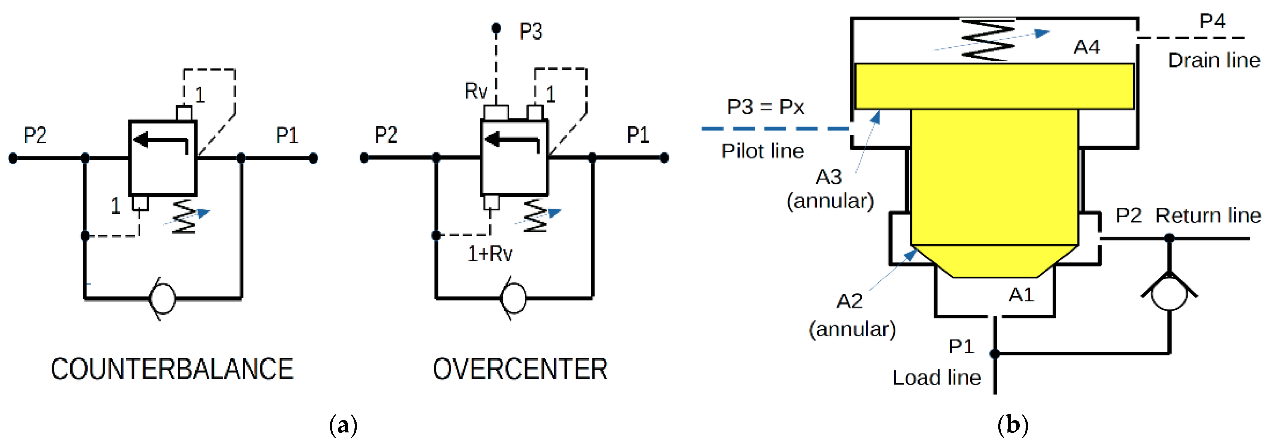
2. Review of Load-Holding Valves

It is believed that the first designs were the work of the Vickers engineers staff in the 1930s and the first valves to appear on the market were developed by Racine. Since then, these valves have received different denominations based on their design and functionality: counterbalance valve, overcenter valve, holding valve, load-control valve, pilot-assisted load-control valve, load-holding valve, and motion-control valves, among others.

The main discussion arises in the use of the names counterbalance and overcenter valve. Counterbalance valves are basically pressure relief valves in combination with a check valve to create a unidirectional back pressure in a hydraulic system to prevent the actuator running away with accelerating loads (see Figure 1a left). The valve poppet is balanced by two pressures and a spring. The force generated by the load pressure (P₁) tends to open the valve orifice, while the spring force and the force caused by the back pressure (P₂) tend to close the valve orifice. The overcenter valve, on the other hand, can be considered in a simplified form as a counterbalance valve with an external pilot line (P₃), being more energy efficient in systems with variable loads (see Figure 1a right). Considering the latest innovations in this valve type, the authors are motivated to look for a more generic name, such as load-holding valve, LHV. Figure 1b shows the scheme of a load-holding valve. Usually, the P₄ connects to the P₂, but P₄ is also left directly to atmospheric reference.

According to Figure 1b, where $A_4=A_1+A_2+A_3$, the force balance on the LHV poppet (Equation (1)) allows for calculating the pressure required to open the valve and starts to move the load. In order to hold the load, the valve cracking pressure (or setting pressure) must be set higher than the load pressure. Because of the hysteresis of the moving parts of the valve (mainly due to friction), there is a difference between cracking and reseat pressure (the pressure at which the valve closes) with the reseat pressure being lower than the cracking pressure. Hysteresis is one of the reasons why the typical LHV valve setting is approximately 30% higher than the load pressure to ensure that the reseating pressure will be high enough to maintain the load.

$$P_1+P_3{R}_v=P_M+P_2\left(R_v+1\right)$$

(1)

where, P₁ is the load pressure, P₃ is the pilot pressure, $P_M=F_{spring}/A_1$ is the spring pressure, P₂ is the return pressure, and R_v is the pilot ratio. The pilot ratio is given by the ratio between the pilot pressure area and the relief area.

$$R_v=\frac{A_3}{A_1}$$

(2)

In Figure 2a, a typical application is shown. A directional valve is used in conjunction with an LHV to control the movement of an actuator. The pilot port of the LHV is connected to the opposite side of the actuator.

The force balance also makes it possible to determine the pressures in the hydraulic cylinder chambers (piston and rod side) as a function of a given load. This balance is established for two situations of the hydraulic cylinder, that is, when the LHV valve is connected to the chamber on the rod side (see Figure 2a) and when it is connected to the chamber on the piston side (see Figure 2b).

For case 2a

$$P_1{R}_c-P_3=P_{Load}$$

(3)

$$R_c=\frac{S_2}{S_1}$$

(4)

$$P_{Load}=\frac{F_{Load}}{S_1}$$

(5)

where, P₁ is the rod side chamber pressure, P₃ is the pilot pressure (equal to piston side chamber pressure), P₂ is the return pressure, and R_c is the hydraulic cylinder section ratio. The sectional area ratio of the cylinder is given by the ratio between the effective sections of rod and piston side.

The load, F, can be considered resistive load (opposite direction for the actuator velocity “sign −”), or overruning load (same direction concerning the actuator speed “sign +”), as depicted in Figure 2.

Assuming that P₂ is very small and combining Equations (1) and (3), the pressures of the hydraulic cylinder chambers can arise from the pressures of the hydraulic cylinder chambers as a function of the spring pressure, P_M, and the equivalent load pressure, P_Load.

$$P_1=\frac{1}{1+R_c{R}_v}{P}_M+\frac{R_v}{1+R_c{R}_v}{P}_{Load}$$

(6)

$$P_3=\frac{R_c}{1+R_c{R}_v}{P}_M-\frac{1}{1+R_c{R}_v}{P}_{Load}$$

(7)

Analogously, for case 2b

$$P_1-P_3{R}_c=P_{Load}$$

(8)

where, P₁ is the piston side chamber pressure, P₃ is the pilot pressure (equal to the rod side chamber pressure), and P₂ is the return pressure.

In the same way, assuming that P₂ is very small and combining Equations (1) and (8), the pressures of the hydraulic cylinder chambers can be expressed as a function of the spring pressure, P_M, and the equivalent load pressure, P_Load.

$$P_1=\frac{R_c}{R_c+R_v}{P}_M+\frac{R_v}{R_c+R_v}{P}_{Load}$$

(9)

$$P_3=\frac{1}{R_c+R_v}{P}_M-\frac{1}{R_c+R_v}{P}_{Load}$$

(10)

Two types of operating curves can be found in the technical documents related to LHVs. On the one hand, the so-called “steady-state operating curve” expresses the load pressure as a function of the pilot pressure (P₃ vs. P₁). Figure 3 shows, for cases (2a) and (2b), the plots of the hydraulic actuator/LHV system based on Equations (1), (2) and (8), corresponding to the steady-state operating curves. The red lines are the characteristic curves of the LHV with different pilot ratios, while the solid black line corresponds to the unloaded hydraulic cylinder, and the dashed gray line corresponds to the hydraulic cylinder with an overrunnig load equivalent to 100 bar. Consequently, intersection point A corresponds to the LHV opening point and intersection point B to the LHV set pressure. This shows the effect of the setting pressure P_M and the pilot ratio R_v on the operation of the LHV. It is significant to note that this representation is used by some manufacturers to highlight differential aspects in the performance of the latest LHV versions, such as the two-stage valve, the multiple pilot ratio (adaptive) valve, and the setting self-adjusting (load match) valve.

Another variant of the operating curve for cases (2a) and (2b) is shown in Figure 4. These plots express the pressures P₁ and P₃ of the system hydraulic actuator/LHV in the cylinder chambers as a function of the equivalent load pressure, P_Load, which is the graphical representation of the two systems of linear Equations (6), (7), (9) and (10). The positive axis direction refers to overrunning loads, while the negative direction corresponds to resistive loads. The red line corresponds to the P₁ pressure and the black line to the pilot pressure, P₃. It can be seen that when the equivalent load pressure decreases, the pilot pressure increases.

The plots in Figure 4 were first introduced by Professor Nicola Nervegna [1] and Professor Luca Zarotti [2]. Ritelli and Vacca used these graphs to evaluate energy aspects in [3], considering the hydraulic power consumption equal to the product of the pressure and the flow rate through the valve. If the flow rate is constant, the hydraulic power is proportional to the pressure in the actuator chamber P₁. Although these graphs have a high conceptual and qualitative value from the energetic point of view, the steady-state operating curves $P_1=f\left(P_3\right)$ shown in Figure 3 can be used to evaluate the power requirements of the hydraulic system with LHV valves, as will be discussed in the following sections.

Table 1. The specifications of the primary hydraulic components of the hydraulic circuit imperative to depict graphs included in Figure 3 and Figure 4.

Cylinder		LHV		System/Load
Piston diameter	100 mm	Pilot ratio	4	Relief valve	250 bar
Rod diameter	63 mm	Setting pressure	325 bar	PLoad (min)	0 bar
Section ratio	0.603	Load max	270 bar	PLoad (example)	100 bar
		Nominal flow	90 L/min

shows the specifications of the essential hydraulic components that make up the hydraulic circuit used. These specifications were to draw Figure 3 and Figure 4, while

Table 2. List of critical points in the diagrams in Figure 4 in bar.

Case (2a)	x	y	x	y
A	Pvlp	Pvlp	250	250
B	(1/Rv)·PM	1/Rv PM	81	81
C	Rc·PM	0	196	0
D	Rc PM	PM	196	325
E	(1/Rv)·PM	0	81	0
F	Pvlp	0	250	0
Case (2b)	x	y	x	y
A	Rc Pvlp	Pvlp	151	250
B	Rc/Rv	1/Rv PM	49	81
C	PM	0	325	0
D	PM	PM	325	325
E	(Rc/Rv)·PM	0	49	0
F	Rc Pvlp	0	151	0

shows the coordinates of the most significant points of the curves shown in Figure 4.

Figure 4. Steady-state operating curves $P_i\left(P_1, P_3\right)=f\left(P_{load}\right)$ for the two cases (2a) and (2b). The meanings of points A–F are defined in Table 2.

Figure 4. Steady-state operating curves $P_i\left(P_1, P_3\right)=f\left(P_{load}\right)$ for the two cases (2a) and (2b). The meanings of points A–F are defined in Table 2.

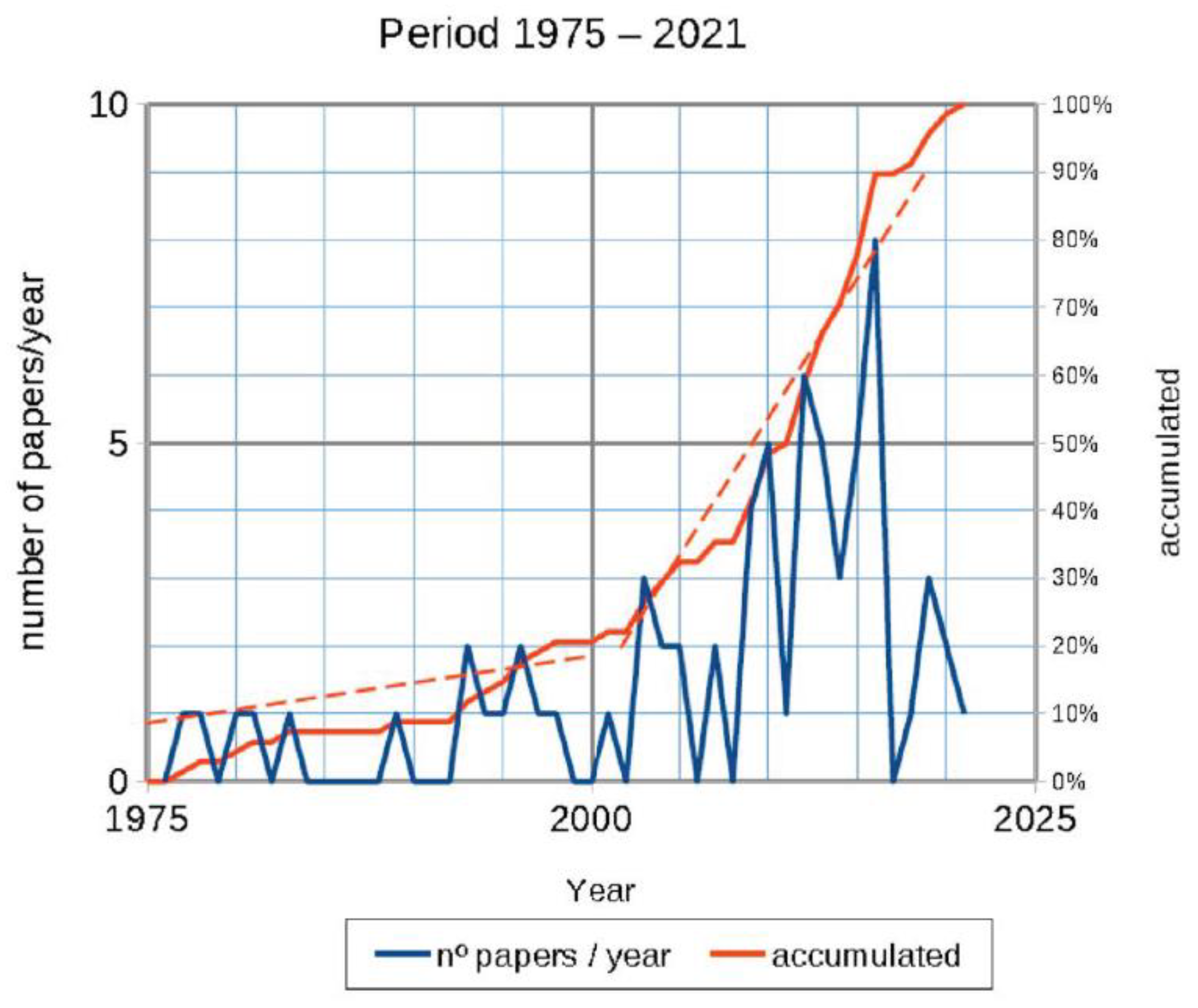
3. The State of the Art

Figure 5 shows a historical compilation of publications published under the following designations: overcenter, counterbalance, and load-holding valves. This list is not exhaustive, but it is sufficient to show the evolution of the scientific and technological aspects. Two clear periods can be observed in this figure: a first period, extending from the beginning to the middle of the first decade of the 21st century, which is characterized by a scientific interest in finding out the causes or origins of instabilities, followed by a second stage focusing on finding designs and/or circuits capable of minimizing or eliminating their effects. In a second period, defined approximately by the last decade, new valve designs appear, modeling is carried out by means of concentrated parameter methods and/or distributed parameter methods, and studies related to energy consumption are found.

3.1. About Instability

As mentioned, the severity of the oscillations is affected by a wide variety of parameters, some of which are hard to predict or change: external load on the actuator, the properties of the mechanical structure, the damping and hysteresis of the LHV, the operator input, as well as the volumes and restrictions in the hydraulic lines. All of these have been subjected to extensive investigations by, among others, refs. [4,5,6,7,8,9,10,11,12,13,14].

It is believed that the inherent stability problem of LHV is due to the fact that there is a phase lag between the pilot pressure and the outlet pressure of the actuator, and oscillations can be reduced by separating the pilot pressure and the actuator inlet pressure [15]. To improve the dynamic response of LHV, ref. [16] suggested that a pressure feedback system can indirectly eliminate oscillations and improve the stability of the hydraulic system. Another novel approach was developed by Sorensen et al. [17], using a low-pass filtered value of the secondary circuit load pressure for the pilot connection of the LHV. From the conceptual point of view, Groof [18] showed a simple criterion that can predict instability. The criterion is based on a third-order equation and indicates when a system is stable or unstable. It focuses only on the hydraulic system, without taking into account the mechanical stiffness of the complete system. When the LHV is mounted on the rod side of the cylinder (in Figure 2a), the criterion used for checking the stability of the system is defined by Equation (11), and when the LHV is mounted on the piston side of the cylinder (in Figure 2b) is defined by Equation (12)

$$\frac{G_{relief}{C}_{hB}}{R_c}>\frac{G_{pilot}}{C_{hA}}$$

(11)

$$\frac{G_{relief}{C}_{hB}}{C_{hA}}>\frac{G_{pilot}}{R_c}$$

(12)

where, G_pilot, gradient of pilot function, describes the opening characteristic as a function of the pilot pressure

$$G_{pilot}=\frac{d{Q}_{throughLHVvalve}}{d{P}_{pilot}}$$

(13)

G_relief, gradient of relief function, describes the opening behavior of the valve depended on the load pressure

$$G_{relief}=\frac{d{Q}_{throughLHVvalve}}{d{P}_{relief}}$$

(14)

C_h, hydraulic capacitance is given by the increase in effective stored fluid volume dV per change in pressure dP. The subscripts A and B indicate the hydraulic conduction and the volume of the cylinder hydraulic chamber on the corresponding side.

$$C_h=\frac{dV}{dP}$$

(15)

By way of illustration and for scenario (2b), the above criterion (Equation (12)) can be expressed by Equation (16).

$$\frac{V_2}{V_1}>R_v{R}_c\left(\frac{2P_1{A}_1}{1+2P_1+k·x_{LHV}-k_f·x_{LHV}·P_1}\right)$$

(16)

where,

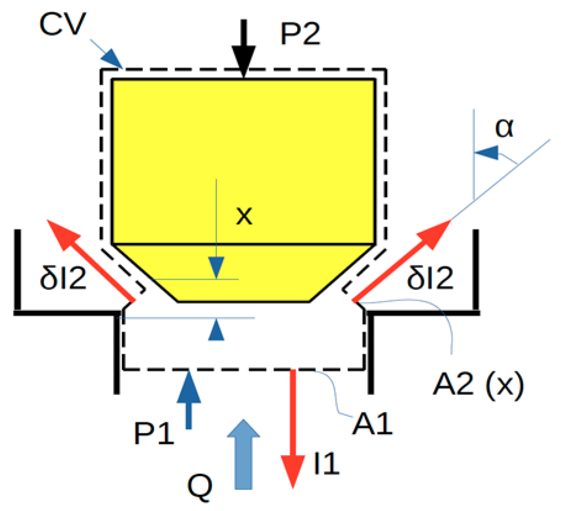
• k, elastic constant of the spring of LHV
• k_f, flow force constant
• V₁, hydraulic cylinder piston side chamber volume
• V₂, hydraulic cylinder rod side chamber volume
• x_LHV, lifting height of the spool/poppet with respect to the seat surface of the LHV

According to the previous paragraphs, the most influential parameters of the stability are the setting pressure and the pilot ratio. A reduction of the pilot ratio results in a more stable operation, but at the cost of a higher pressure level and thus higher energy consumption, see ref. [3]. This is especially significant for small external loads. Adding damping when designing the hydraulic circuit is another proven approach. By increasing volumes, adding orifices, using logic valves, etc., more damping is introduced into the system. Special attention has been devoted to the pilot line. By manipulating the pressure in different ways on the LHV pilot port line (adding delays, creating a difference in the path back and forth), positive effects have been achieved. Sciancalepore and Vacca [19] proposed a solution by using LHVs to control the actuator speed while also reducing energy consumption. It consists of controlling the pilot port of the LHV through an external pressure source (adjustable pilot). Two different control strategies are presented: the “Smart LHV”, where the LHV does not control the actuator velocity but it minimizes the system pressure; and the “Smart System” that uses the LHV to efficiently control the actuator velocity during overrunning load conditions.

3.2. About Modeling

Most of these investigations are related to modeling the steady-state and dynamic characteristics of load-holding valves in the time and frequency domains using a lumped parameter approach. However, most attempts to establish physical or semi-physical models of such valves have encountered many challenges, e.g., related to friction and resulting hysteresis, non-linear discharge area characteristics, varying discharge coefficients, and varying flow forces.

Today, there are several commercially available software packages such as MATLAB/Simulink™ (The MathWorks, Inc., Natick, Massachusetts, United States), AMESim™ (Siemens AG, Munich, Germany), Dymola™ (Dassault Systèmes, Paris, France), Maple/MapleSim™ (Waterloo Maple Inc., Waterloo, AB, Canada), and 20-Sim™ (Controllab Products B.V., Enschede, The Netherlands) that make work much more manageable. These packages may be classified into two different modeling approaches: a simple semi-physical model and a non-physical model (black box).

In the first approach, static modeling method based on force balance and the Bernoulli orifice pressure–flow equation is used to achieve the load velocity control ability of the valve. It does not take phenomena like friction and flow forces into account. In other cases, the dynamic modeling method is based on Newton’s second law and fluid continuity equation. In both cases, experimental verification was required. In the second approach, the model uses two different pressure ratios to compute the flow through the valve together with a number of parameters that must be experimentally determined. Despite this, LHVs are rarely modeled accurately due to the effort required to obtain basic model parameters and the complexity involved in identifying equations for flow forces and friction.

Computational fluid dynamics (CFD) may be used to provide insight into some of these phenomena, but often experimental work and semi-physical or non-physical modeling approaches are required for time-domain simulation. Very interesting and to highlight are the works of refs. [14,20].

3.3. About Energetic Aspects

The energetic analysis of fluid power systems is becoming a requirement of machinery manufacturers, taking into account the trend towards the electrification of machines and the limited battery capacity. Many researchers are involved [21,22,23,24,25], and some are specific to studying the different hydraulic load retention systems in mobile and industrial applications [15,26,27].

Ritelli and Vacca [3] focused on the analysis of LHV energy savings. They quantified the energy consumption of LHVs with different pile ratios, showing that in a crane application, it is possible to achieve 59% energy savings with high pile ratios.

Regarding the energy efficiency of LHVs, there are some relevant previous efforts. LHVs with external and mixed control types were considered by ref. [13]. Significant examples are also the LoadMatch™ model, recently commercialized by Sun Hydraulics, which dynamically changes the valve setting as a function of the load pressure. In contrast, other works focus on introducing an external control to the LHV to influence its opening based on the instantaneous loading conditions. The most important contribution in this direction is the work in ref. [17], which proposed to use an auxiliary hydraulic circuit to control the pilot of the LHV, and ref. [28], which presented a method to control the pilot port of the CBV through an external pressure source (adjustable pilot). For both cases of “Smart CBV” and “Smart System”, remarkable energy savings of 75% and up to 90%, respectively, were observed.

Despite scientific and technological advances reported and the wide variety of models and algorithms, it can be said that the use of this type of valve is far from easy. This wide range of tools is often not available to application engineers. In addition, the use of these tools still require a high level of application-specific knowledge. The impact outside academia remains limited. One reason may be that the design of hydraulic systems depends to some extent on the application.

In this paper, the authors highlighted the importance of understanding how LHVs work, not only in the critical opening condition but also outside of this condition, with the aim of helping to select the most suitable valve for the application according to its characteristics (extracted from the corresponding technical catalogs). Of course, experimentation is the best way to judge the system’s power consumption but, the availability of a simple graphical method in the course to estimate the impact of the LHV on the overall power consumption may be very useful.

Of course, experimentation is the best way to judge the system’s power consumption. However, the availability of a simple graphical method in the course to estimate the impact of the LHV on the overall power consumption may be very useful. In the next section, a brief background overview of the different types of performance curves is presented.

3.4. Performance Curves

Choosing the satisfactory LHV valve for a specific application is a challenging task. In order to apply a LHV correctly, it is crucial to understand how it works and to have sufficient technical information about its performance. After carefully analyzing the catalogs and other types of technical documents (release and technical papers, handbooks, user’s manual, worksheets, prospectus, or brochures) the following comments can be summarized:

a

They all provide a simple and generic description of how it works, symbols, valve cavity, specifications or technical data, and some performance graphs or characteristic curves.

Typical technical data include maximum operating pressure, setting pressure (cracking pressure) interval, nominal flow, pilot ratio, internal leakage, and hysteresis, among others.

b

Although graphical presentations of performance should help viewers quickly and easily understand the critical information, there is no unanimous agreement on which are the most appropriate. Of the different ways of expressing its performance, the next conditions may be pointed out:

i

Pressure drop in pilot operation condition (valve fully opened by the pilot pressure), (from port 1 to port 2, see Figure 1).

ii

Pressure drop in check valve operating condition (free flow) (from port 2 to port 1) and

iii

Pressure drop in pressure relief working condition (valve opened by the load). Unfortunately, some technical documents or specification sheets do not provide this minimum information, which is necessary for applying LHVs in a system.

c

Generally, the curves shown at the end of Section 2 of this document and in Figure 3 and Figure 4 are not usually included in the catalogs, but only in technical papers and to highlight the significant improvements in the performance of different valves.

4. Graphic Method to Estimate the Power Balance

The method is attractive because only the pressures in the three ports and the relief function curve of the valve are sufficient to evaluate the power consumption. The method has been inspired by the work done at the Agder University, Norway, led by Prof. M. Hansen [11]. It consists of a simple semi-physical model.

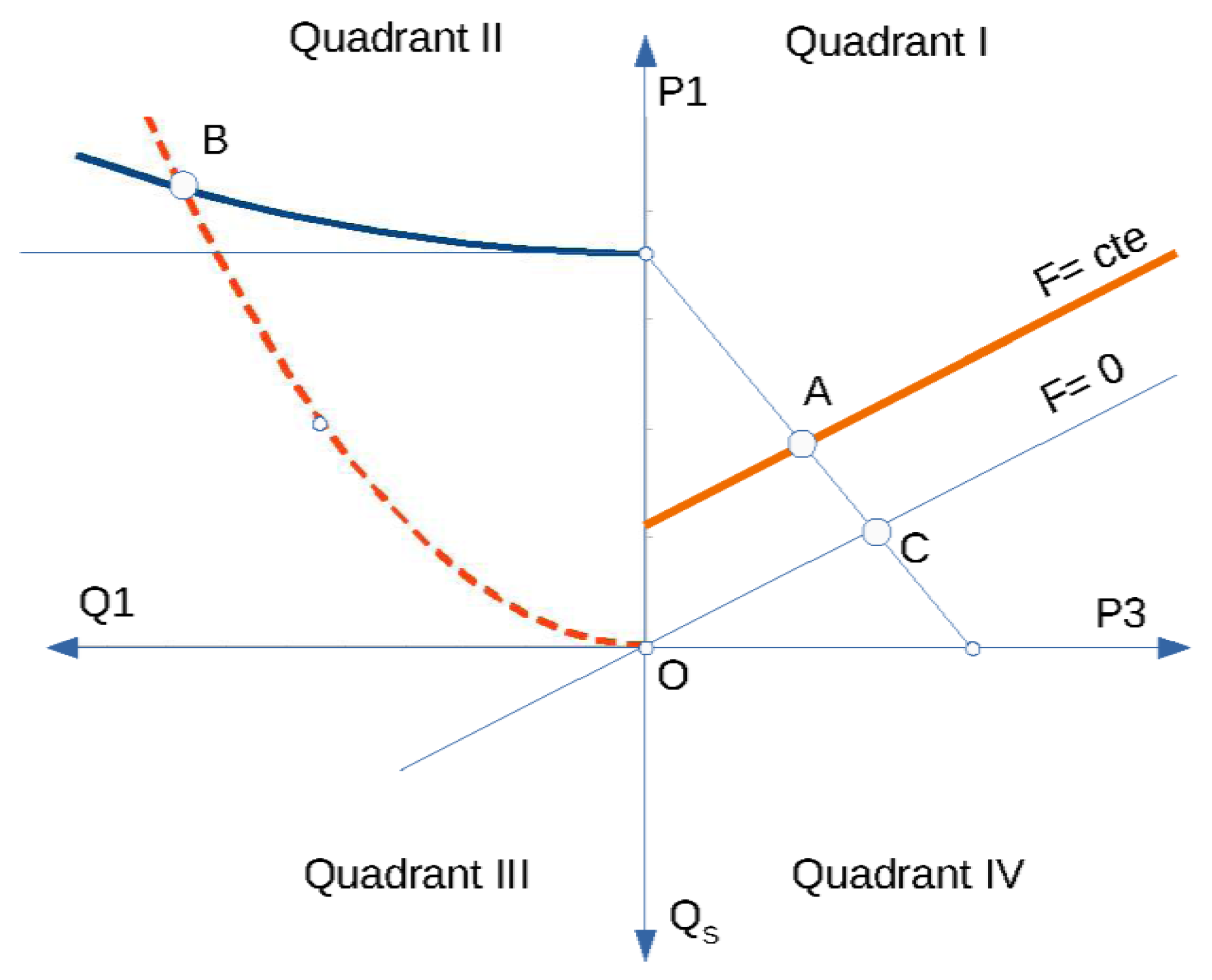
4.1. Description of the Four-Quadrant Diagram

For the description of the graphical method, the four-quadrant diagram of the Cartesian plane is a good description of the proposed method (Figure 6). The following variables are represented on the axes of this diagram:

• x-axis (+): pilot pressure (P₃) in bar which corresponds to the pressure that prevails in the actuator rod chamber
• x-axis (−): flow through the load holding valve (Q₁) in L/min, equal to the flow leaving the piston side actuator chamber
• y-axis (+): load pressure (P₁) in bar, corresponding to the pressure in the actuator piston chamber
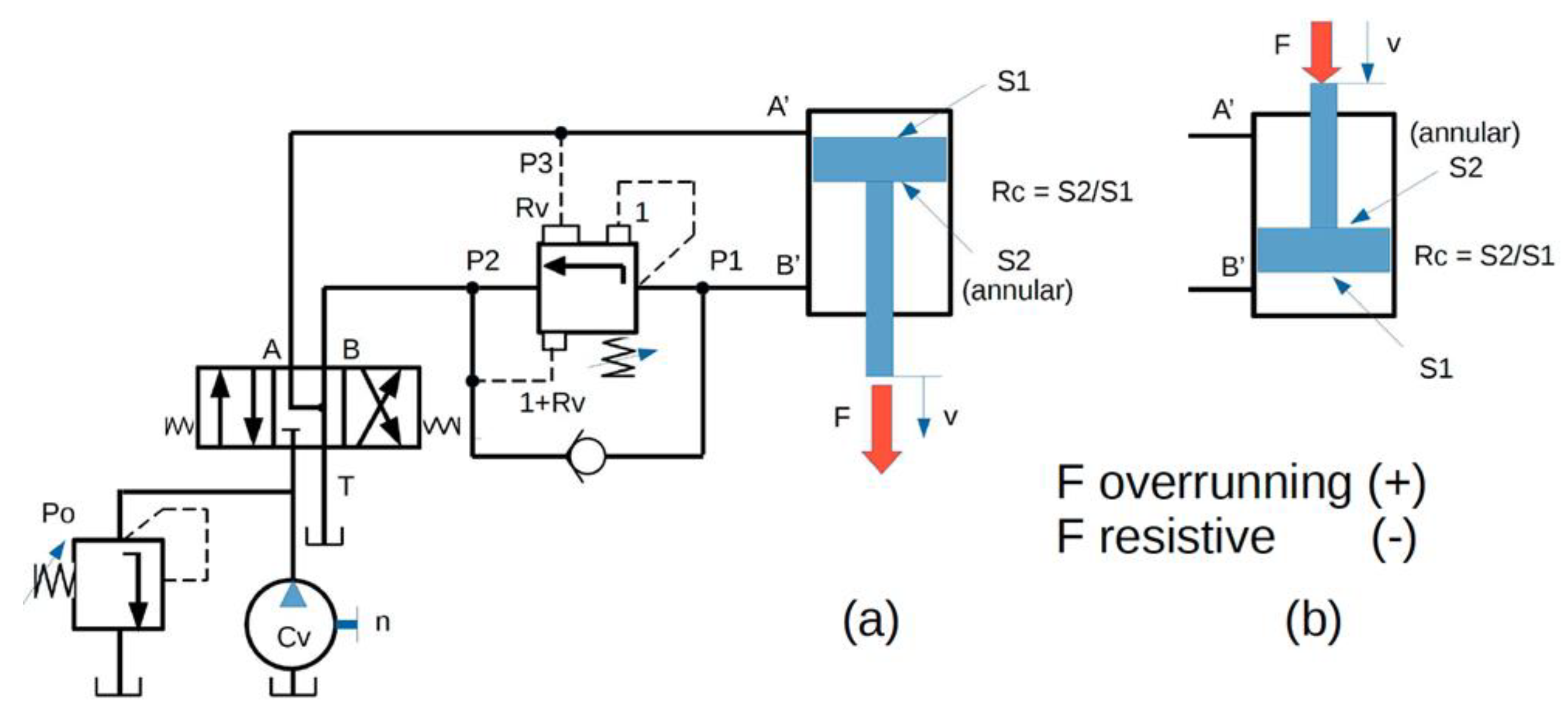
• y-axis (−): flow rate entering the piston side actuator chamber (Q_S) in L/min according to the configuration of the hydraulic circuit shown in scenario (2b), Figure 2.

The four-quadrant diagram allows us to plot the characteristic curves of an actuator and holding valve as follows:

-

First quadrant “I”: Upper right region. It is used to represent the characteristic curve of the hydraulic actuator and the characteristic curve $P_1=f\left(P_3\right)$ of the load-holding valve.

-

Second quadrant “II”: Upper left region. It is used to show the characteristic curve of the load holding valve acting as a pressure-limiting valve (relief function).

-

Third quadrant “III”: Lower left region. It is used as an auxiliary two-dimensional space.

-

Fourth quadrant “IV”: Lower right region. It is used as an auxiliary two-dimensional space.

Alternatively, it can be used to depict the characteristic curve of the load-holding valve that expresses the pilot pressure (P₃) as a function of the flow rate (Q₁) through the load-holding valve for a predetermined load pressure value (P₁)

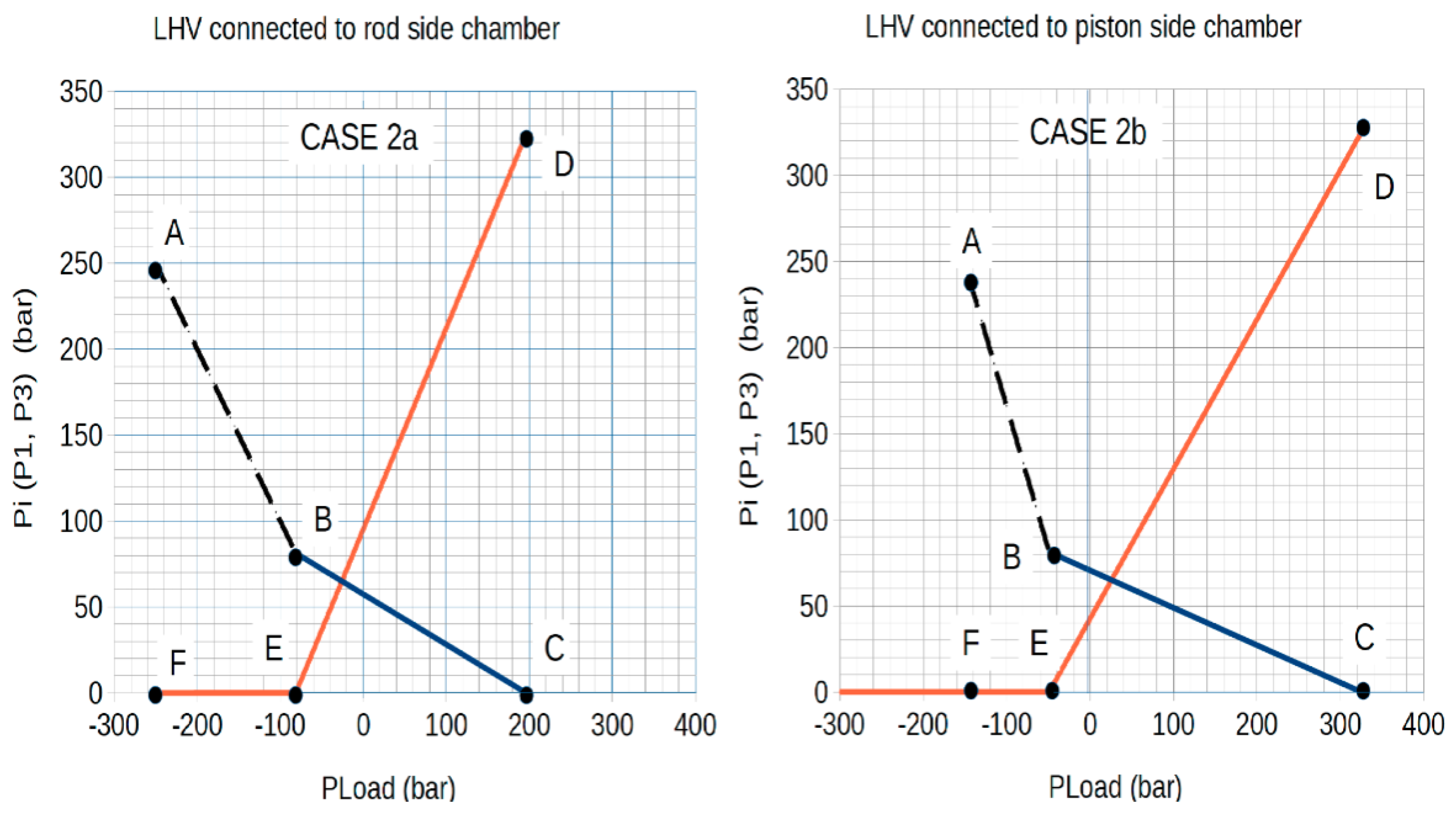
4.1.1. Steady-State Operating Curve and Hydraulic Cylinder Characteristic Curve

Equations (1) and (3) have been plotted in quadrant I. The intersection between the two curves gives the operating point of the hydraulic system (actuator/LHV valve) when the cylinder is subjected to a load, overrunning or resistive, as in Figure 3.

4.1.2. Characteristic Curve $P_1=f\left(Q\right)$ of an LHV Valve Acting as a Pressure Limiting Valve (Relief Function)

Considering the simplified diagram of the holding valve poppet shown in Figure 7 and assuming that P₃ is not working and the flow is in a steady-state and incompressible fluid (ρ is constant), the application of the principle of conservation of momentum to the control volume allows us to write:

$$I_2-I_1=P_1{A}_1-P_2{A}_2-F_{solid-fluid}$$

(17)

$$F_{fluid-solid}=-F_{solid-fluid}$$

(18)

where: $P_1{A}_1$ and $P_2{A}_2$ denote the net force due to the pressure distribution in the inlet and outlet sections, respectively, I₁ and I₂ are the momentum fluxes of the flow entering and leaving the control surface,

$$I_1=\frac{\rho Q^2}{A_1}$$

(19)

$$I_2=\frac{\rho Q^2}{A_2\left(x\right)}\cos \left(\alpha \right)$$

(20)

where

$$A_2\left(x\right)=\pi ·d·sen\left(\alpha \right)·x=K_2·x$$

(21)

$$K_2=\pi ·d·sen\left(\alpha \right)$$

(22)

and F_fluid-solid is the force on the poppet exerted by the fluid.

Applying Newton’s second law of motion to the valve poppet (considered a free solid)

$$F_{fluid-solid}-(F_{spring}+M_{solid}g)=M_{solid}\dot{v}$$

(23)

Accepting an equilibrium position defined by the distance, x, considering that M_solid is negligible then:

$$F_{fluid-solid}=F_{spring}$$

(24)

$$F_{spring}=K_1\left(x+x_0\right)$$

(25)

where, K₁ is the constant of the spring

$$F_{precompresion}=K_1{x}_0$$

(26)

$$P_M=\frac{F_{precompresion}}{A_1}$$

(27)

Combining the previous Equations (17)–(27), it follows that the relief function curve

$$P_1=P_M+\frac{K_{spring}}{A_1}x+K_2{Q}^2$$

(28)

with

$$K_2=\frac{\rho }{A_1^2}-\frac{\rho }{A_1·\left(\pi d\right)·x·\tan \alpha }$$

(29)

On the other hand, for a predefined distance between poppet and seat surface, the flow rate can be calculated by the equation

$$Q_{out}\left(y,P\right)=K_2·x·C_d·\sqrt{2\frac{P_1}{\rho }}$$

(30)

or alternatively

$$P_1=K_3{Q}^2$$

(31)

with

$$K_3={\left(\frac{1}{K_2·x·C_d·\sqrt{\frac{2}{\rho }}}\right)}^2$$

(32)

In quadrant II, see Figure 8, the relief function curve (Equation (28)) and the flow rate curve (Equation (31)) are represented (not scaled). The point of intersection between the two curves (point B) indicates the operating point of the LHV acting as a relief valve; that is, the valve opens at pressure P and allows fluid flow Q.

4.1.3. Power Balance Applied to the Actuator/LHV Hydraulic System

Before explaining how the power balance is proposed, it is helpful to explain the different curves shown in the four-quadrant diagram (Figure 8), as well as the points that are considered most representative:

-

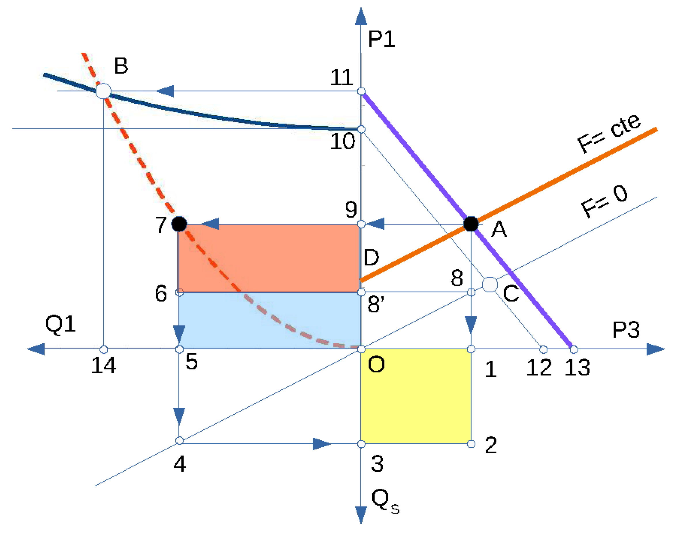
Curve 10–12: characteristic curve P₁ = f(P₃) of the LHV valve in the static balance position (closing condition). It corresponds to the representation of Equation (1). Load force $F_{load}=0$

-

Curve 11–13: characteristic curve P₁ = f(P₃) of the LHV valve in the permanent regime when a flow rate Q₁ flows through the valve, as a consequence of the opening of the obturator by the action of pressure P₁ and pilot pressure P₃. Load force constant $F_1>0$

-

Curve O–C: characteristic curve P₁ = f(P₃) of the hydraulic actuator when it is subjected to zero force. It corresponds to the representation of Equation (3).

-

Curve D–A: characteristic curve P₁ = f(P₃) of the hydraulic actuator when it is subjected to an overrunning force, F = constant.

-

Curve 10–B: characteristic curve P = f(Q) of the LHV valve acting as a pressure limiting valve (relief function). See Equation (28).

-

Curve O–7–B: LHV poppet pressure drop in the open position as a result of the shutter opening due to the action of the pressure P₁ and the pilot pressure P₃. See Equation (31).

Assuming that the operating point of the hydraulic system (hydraulic actuator/LHV valve) is defined by point A, that is, the intersection of curves (11–13) and (D–A), this point corresponds to the operating point of the LHV when a flow rate Q₁ flows as a result of the opening of the obturator under the action of pressure P₁ and pilot pressure P₃, thus defined by the coordinates (P₃, P₁).

Other points of interest are:

-

point 7: This point is defined by the coordinates (Q₁, P₁), intersection of the curve (0–B), with the line of constant pressure equal to P₁.

-

point 5: defined by the coordinates (Q₁, 0)

-

point 1: defined by the coordinates (P₃, 0)

-

point 3: defined by the coordinates (0, Q_S)

Based on the hydraulic circuit (e.g., scenario 2b) outlined in Figure 2, the following powers involved in movements are defined:

N_M power due to the movement of the actuator as a consequence of being subjected to the overruning force F.

$$N_M=F_{overrunning}.v_{actuator}$$

(33)

N_S, power supplied by the pump feeding the hydraulic actuator chamber on the rod side

$$N_S=P_S{Q}_S=P_{S\left(:point 1:\right)}{Q}_{S\left(:point 3:\right)}$$

(34)

N_LHV, power related to the fluid flow through the LHV valve as a result of the combined action of pressure P₁ and pilot pressure P₃

$$N_{LHV}=P_1{Q}_1=P_{1\left(:point 9:\right)}{Q}_{1\left(:point 5:\right)}$$

(35)

A simple power balance allows us to establish the following equation:

$$N_{LHV}=N_S+N_M$$

(36)

N_S power is defined by the rectangle (O123) (yellow area), where side O3 has magnitude Q_S and side O1 has magnitude equal to P₃. Note that the area (O123) is equal to the area (O568’). Using the hydraulic actuator curve (for condition $F=0$) extended from Quadrant I to Quadrant III, represented by the “40C” line, the following relationships are established:

$$P_{1\left(:point 8^{\prime }:\right)}=R_c{P}_{3\left(:point 1:\right)}$$

(37)

$$Q_{1\left(:point 5:\right)}=\frac{Q_{S\left(:point 3:\right)}}{R_c}$$

(38)

multiplying Equations (37) and (38), it turns out

$$P_{1\left(:point 8^{\prime }:\right)}{Q}_{1\left(:point 5:\right)}=P_{3\left(:point 1:\right)}{Q}_{S\left(:point 3:\right)}$$

(39)

Equation (39) highlights the aforementioned equality, that is the area (O568’) = area (O123). On the other hand, note that the area of the rectangle (O579) (A_Blue + A_Red), where side O5 has magnitude Q₁ and side O9 is equal to P₁, represents the power N_LHV, i.e., the power related to the fluid flow through the LHV valve. Then, by virtue of Equation (36), it can be deduced that the area of the rectangle (6798’) (A_Red), represents the power due to the movement of the actuator as a consequence of being subjected to the overrunning force F.

Based on these equations, the ratio ϕ is defined between the power provided by the pump and the power related to the flow through the LHV valve, see Equation (40). This power ratio is an index that indicates the percentage of the pump power needed to open the LHV valve and, therefore, an index of the energetic goodness of the LHV valve.

$$\varphi =\frac{N_S}{N_{LHV}}=\frac{area\left(O{568}^{\prime }\right)}{area\left(O579\right)}=\frac{Are{a}_{Blue}}{\left(Are{a}_{Blue}+Are{a}_{Red}\right)}$$

(40)

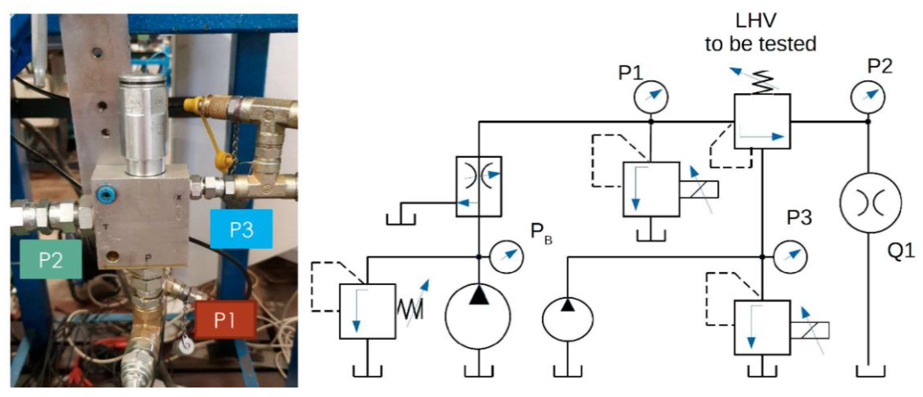
5. Experimental Validation

5.1. Lab Testing

To validate the proposed methodology, first of all, the performance of an LHV valve was tested. Specifically, the reference valve tested at the LABSON Laboratory (Terrassa-Barcelona) was the LHV-4 valve (note: there was no particular reason for the choice, only its availability in the laboratory). Figure 9 shows the diagram of the hydraulic circuit used.

Figure 10 presents the results obtained. Figure 10a shows the steady-state operating curve of LHV valve, while Figure 10b shows of relief function curve. On the one hand, the relief functions with setting pressure of 150 and 250 bar are shown. These curves were evaluated based on the adjustment curves shown in Figure 10a. On the other hand, the relief curve with setting pressure 100 bar, obtained by varying the pressure P₁ with the help of a proportional pressure relief valve, showed its hysteresis phenomenon.

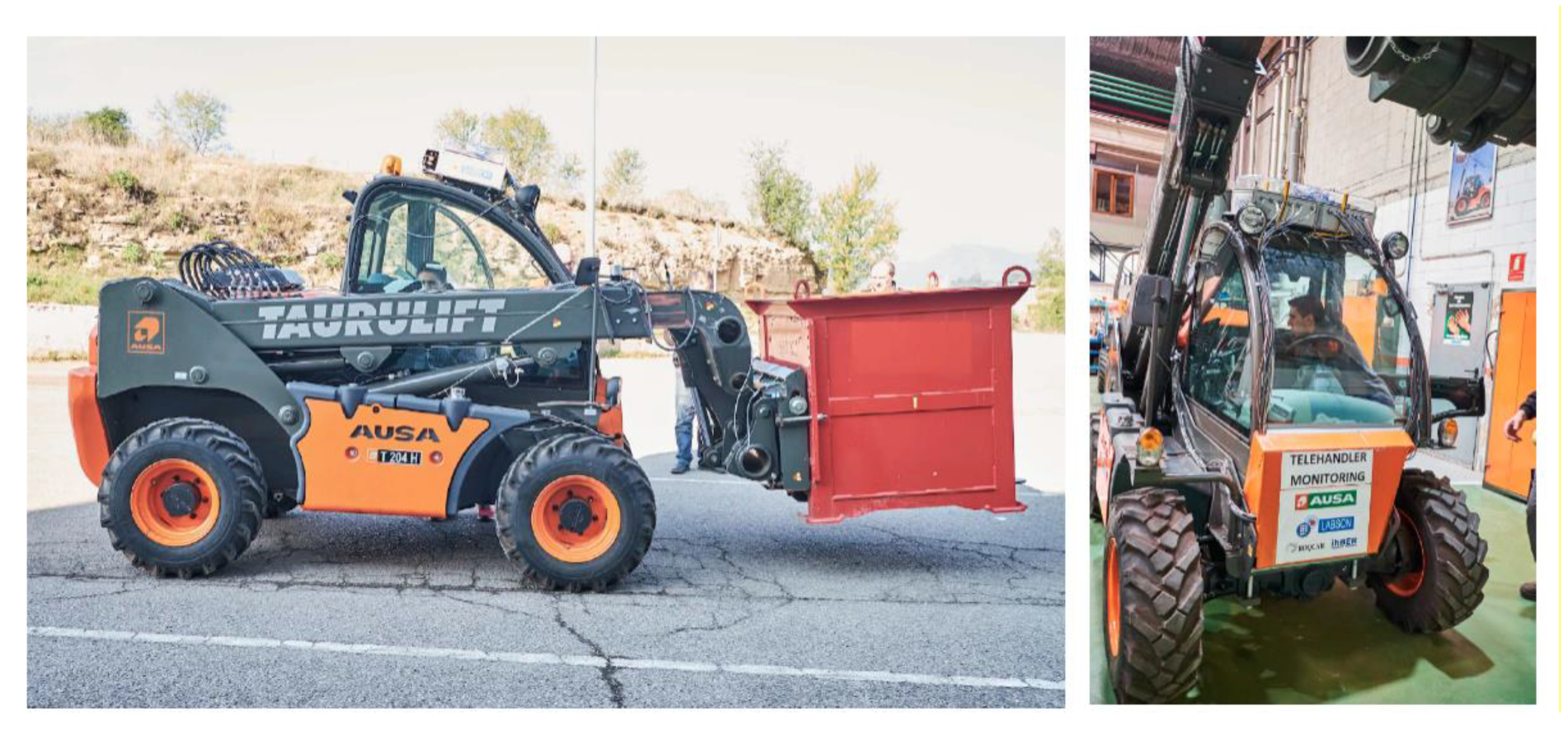
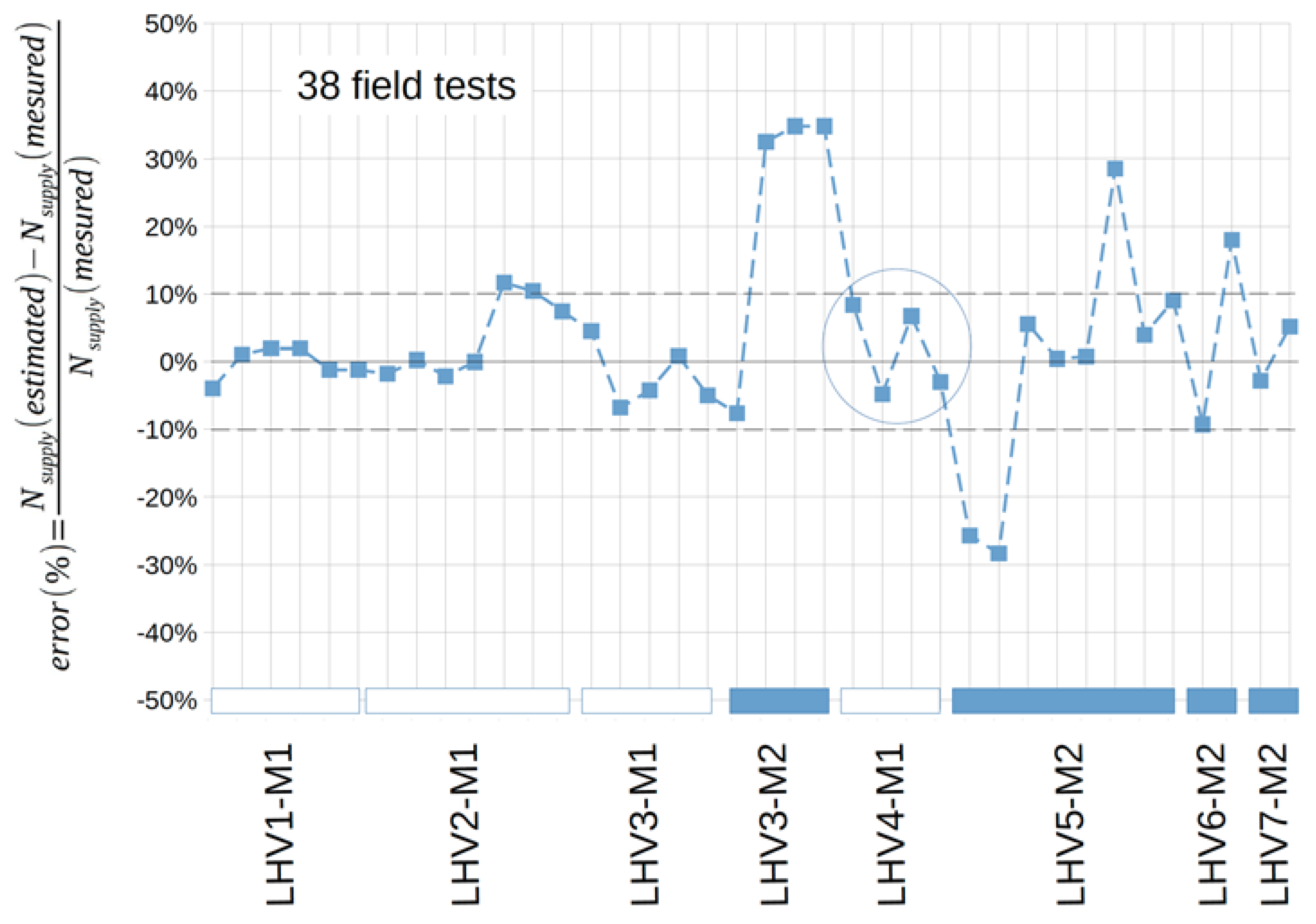
5.2. Field Testing

This section describes the experimental tests performed to validate the methodology proposed in the previous section. Several tests were performed on the hydraulic lifting cylinder of a telescopic handler (called M₁). For the first series of tests, the M₁ telehandler was equipped with the LHV4-M₁ valve, the characteristics of which are well known (Figure 10), replacing the original valves of the commercial version.

Figure 11 shows panoramic images of the experimental tests carried out. The tests were carried out with different load conditions of the telehander.

The hydraulic cylinder was actuated by means of a manual directional control valve. The field test was equipped with multiple pressure sensors, a flow sensor, and a cylinder position sensor. Displacement and angle sensors were also fitted to the boom.

Sensor data acquisition and electronic actuation were carried out with the help of a multi-axis motion controller RMC200, equipped with input and output modules (Delta Computer Systems). It is easy to use, and the software provided with it has powerful plotting capabilities.

Sensors and their main characteristics are listed in

Table 3. List of main characteristics of used sensors.

Magnitude	Manufacturer	Model	Range	Accuracy
Pressure	WIKA	MH2	0–250/0–400 bar	>0.5% span
Flow	HYDAC	EVS3199TF	6–60 L/min	>2% act. val.
Position	Micro Epsilon	WDS-1500_PS60-SR-U	0–1500 mm	>+/−1.5 mm
Angle (tilt)	SICK	TMM 56E-PMH045	+/−45°	+/−0.3°
Temperature	Omega	PT100	10–100°	>0.36 °C

. Calibration values were obtained from the manufacturer’s information and from comparison with a standard when the manufacturer’s information was not available. All values were checked in preliminary tests. Sensor values were measured and recorded at a frequency of 1 kHz. Higher rates were not considered necessary for the energy analysis. Digital filtering at 100 Hz was required for the calculation of the speeds, especially with the angle sensor. The data were processed with commercial software (DIAdem, Excel) to calculate the total energy consumption.

Figure 12 shows the results obtained with machine M₁ in which a 90 × 50 hydraulic cylinder and the LHV4 valve were installed to move the telescopic arm. Figure 12a shows the temporal history of the load pressure P₁, the return pressure P₂, and pilot pressure P₃, together with the hydraulic cylinder position x₁ and pump flow Q_S companion. It is observed that there is a time interval in which the values P₁, P₂, P₃, and Q₁ remained essentially constant, which corresponds to the downward cylinder movement, x₁, and, consequently, to the time interval in which the valve is working. The companion Figure 12b shows the working pressure space of rod side P₁ versus the pilot P₃ pressures, respectively. The average values are represented by a small circle in Figure 12a,b.

Procedure

The method is presented over the description set out in Figure 13 with real values (and Figure 8 as reference).

Actions to be carried out over the first quadrant:

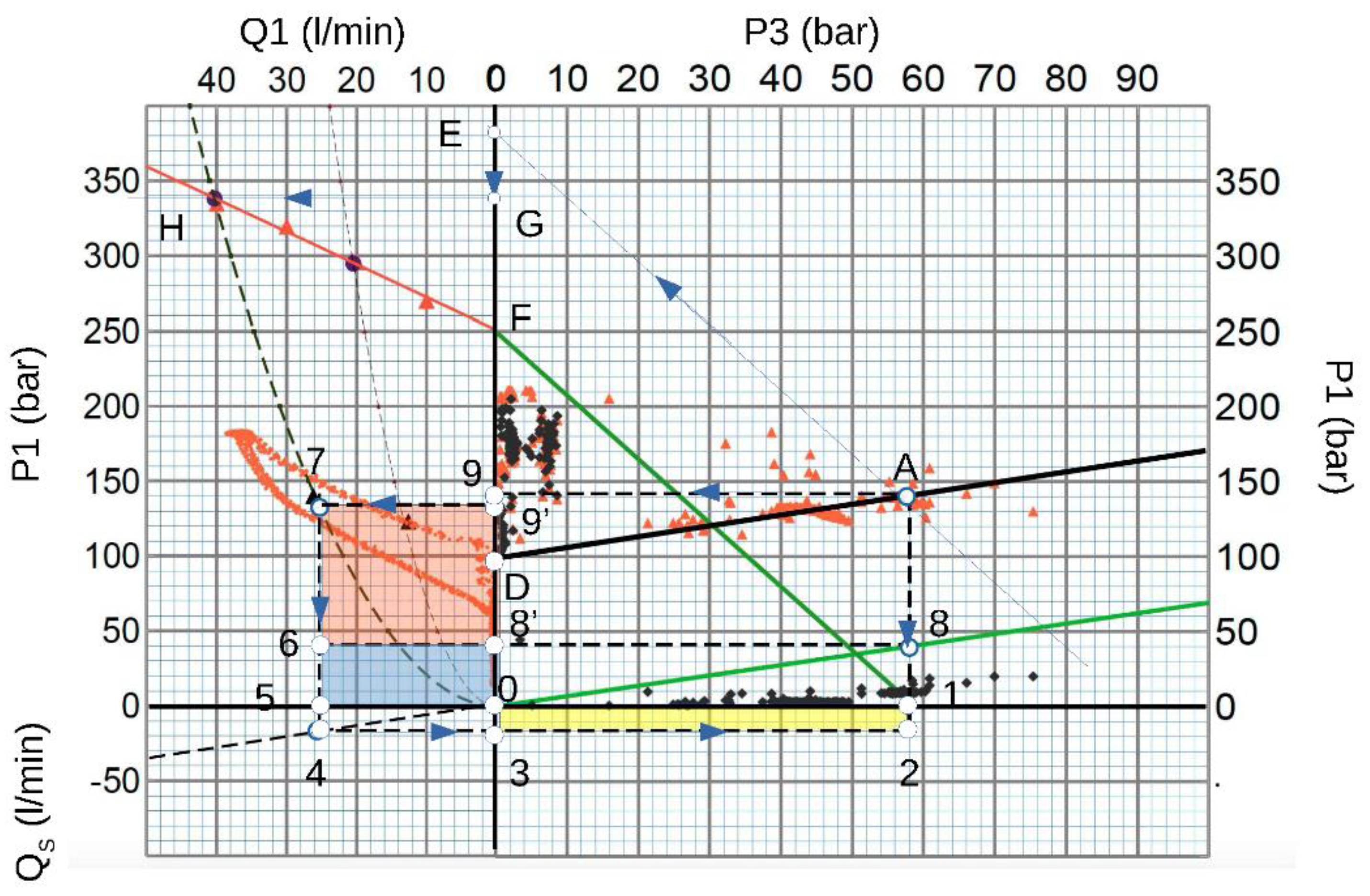
• Plot the working point A (e.g., P₁ = 142 bar and P₃ = 58 bar);
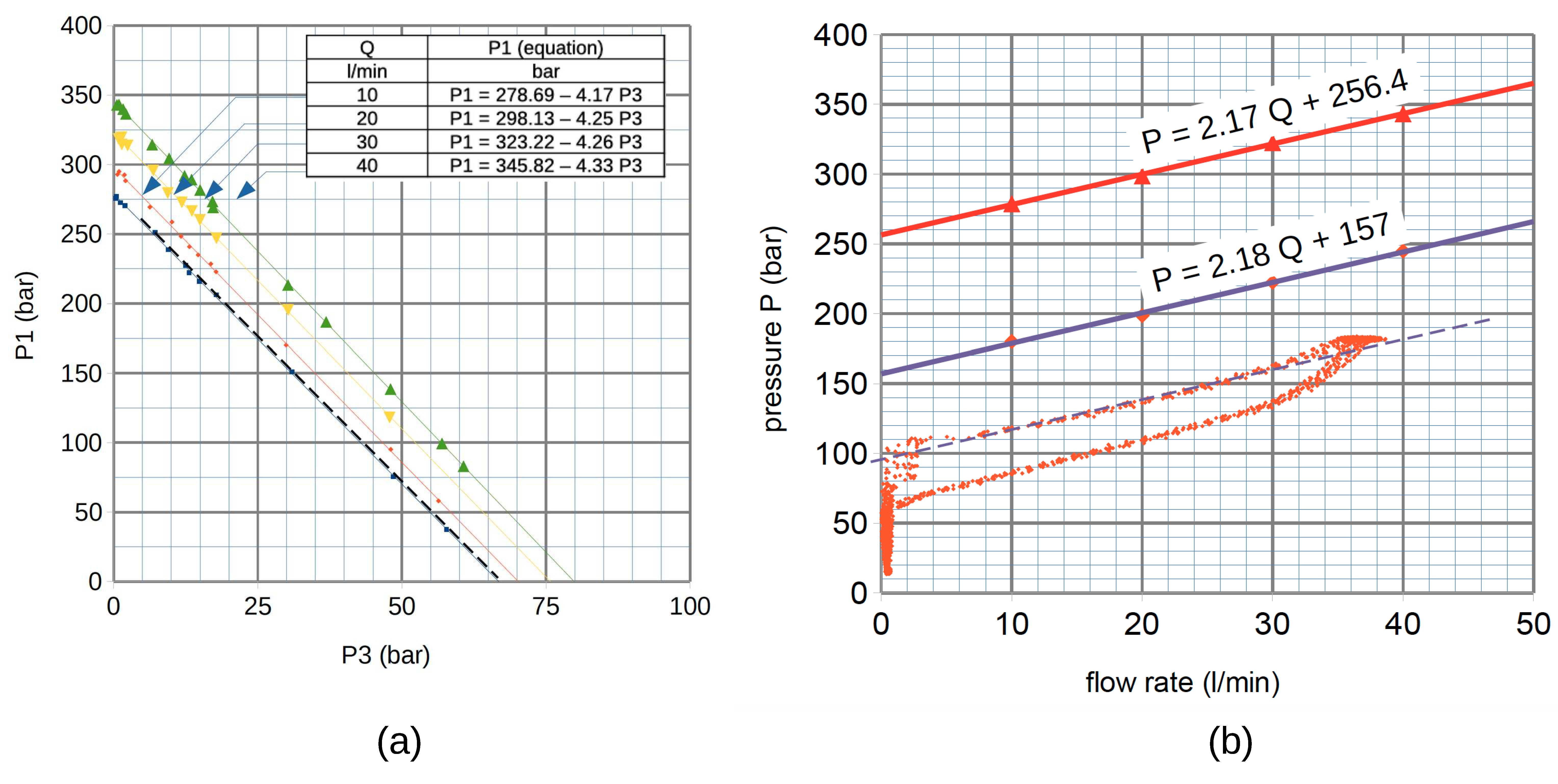
• Plot LHV curve based on its setting point P_m = 250 bar and the pilot ratio 4.25 as it is shown in Table 1 (e.g., straight-line 1F);
• Plot an auxiliary line parallel to 1F at the A point projecting it to the pressure axis (e.g., E point);
• Calculate the effect of the return pressure using the equation P₂·(R_v + 1), which is represented by the segment EG. G point represents P_M pressure shown in Equation (1);
• Trace a horizontal line crossing at A point to obtain the working pressure (e.g., point 9);
• Obtain the differential pressure P₁-P₂ by plotting 9′ position (e.g., segment length between 0–9′).
  Actions in the second quadrant:
• Plot the relief LHV function curve taking the setting pressure as 250 bar (e.g., the experimental curve shown in Figure 10b);
• Draw a horizontal line starting at G and crossing the LHV function curve (e.g., H point is obtained). Therefore, the K₃ constant can be calculated from Equation (3) obtained using H coordinated, $K_3=\frac{P_H}{Q_H^2}$;
• The parabolic performance following Equation (31);
• Trace a horizontal line across 9′ to obtain the coordinates of intersection with the parabolic curve OH to bring point 7, which corresponds to the orifice working conditions;
• Draw a vertical segment from point 7 to the flow axis to obtain the flow Q₁ through the valve (point 5);
• Extend the cylinder actuator characteristic curve from the first quadrant to the third quadrant (segment “04”, as an extension of segment “08”);
• The pump flow rate Q_S is represented by point 3, which is calculated from point 4 by crossing the vertical axis;
• Extend line “4–3” to the intersection with the vertical line through point 1, obtaining point 2;
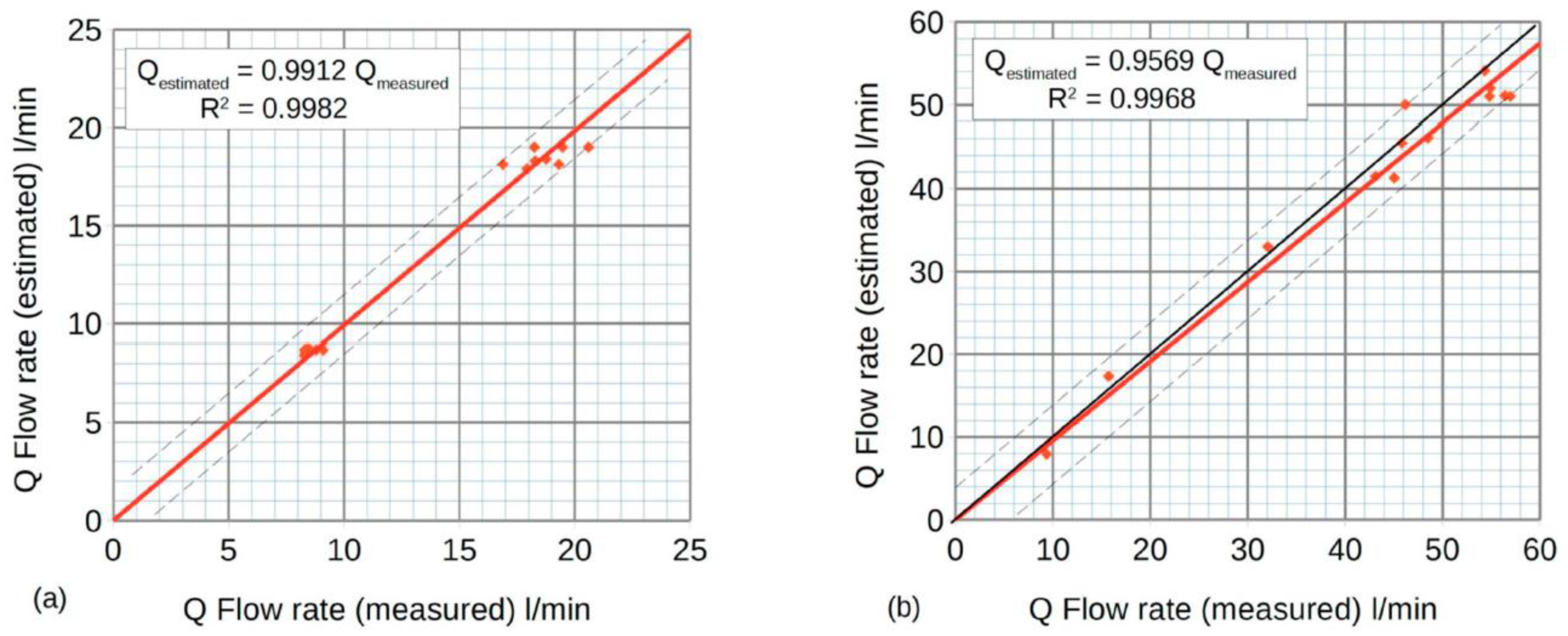
• The graphics method provides flow rate (represented by points 3 and 5 compared with experimental ones, as shown in

  Table 4. Working values.

  			Go down Slow	Go down Fast
  load pressure	P1	bar	132	142
  return pressure	P2	bar	3	9.21
  pilot pressure	P3	bar	42	58
  supply flow	QS	l/min	9	18
  valve flow	Q1	l/min	13	26
  setting pressure	Pm	bar	250	250

  ).

Power ratios ϕ can be obtained applying Equation (40).

-

“(0123)” area represents the power, N_S (yellow area)

-

“(0568′)” area has an identical area of “(0123)” (blue area)

-

“(679′8′)” area is equivalent to the power load, F·v (red area)

-

“(0579′)” area is the power dissipated in the valve, $N_{LHV}=P_1{Q}_1$, which is equal to the sum of “(0568′)” and “(679′8′)”

The yellow area, identical to the blue area, shows that using LHV valves in a hydraulic system introduces additional energy consumption.

To conclude this research work, it is essential to apply and validate the proposed methodology in more cases. For this purpose, two models of telehandlers (M₁ and M₂) were equipped with seven different LHV valves. The mixed sets of valves and machines were distinguished with LHV_i-M_j where i = {1 … 7} and j = {1,2}. The relevant data, setting pressure, and relief characteristic curve were obtained from the commercial catalogs of the valves.

Figure 14 shows the high correlation between the flows estimated by applying the proposed method and the experimental tests carried out in the field with the two machines presented and the set of seven valves used. The high correlation measured through the coefficient R₂ ≈ 0.99 is notable. Taking into account that the proposed method allows estimating the flows and powers involved in the operation of the hydraulic cylinder/holding valve system, it seems reasonable to compare the calculated values with the actual values measured in the experimental tests in order to obtain the accuracy of the method. The estimated and measured flow rates for machine M₁ are shown in Figure 14a, where the dashed lines define an error range of ±7.5%. On the other hand, the values for the machine M₂ are shown in Figure 14b, where the dashed lines define an error range of +8%/−12%.

Figure 15 shows the power ratio, ϕ, as a function of the net force to which the lifting cylinder is subjected for machines M₁, Figure 14a, and M₂, Figure 14b.

Figure 16 shows the order of magnitude of the errors made in the estimation of power according to the following definition:

$$error(\%)=\frac{N_{supply}\left(estimated\right)-N_{supply}\left(mesured\right)}{N_{supply}\left(mesured\right)}$$

(41)

6. Conclusions

In this paper, the authors highlighted the importance of understanding how LHVs work in the critical opening condition. Outside of this state, it helps select the most suitable valve for the application according to its characteristics.

Going deeper into the knowledge of these valves requires the use of tools (software and models). Still, it involves a high level of application-specific knowledge (mainly done in academia). On the contrary, the methodology presented in this paper is an ad hoc methodology ready to use for an end-user.

The primary method’s advantage is that the information provided by a catalog and the pressure readings in the three ports of the valve is sufficient to estimate the power ratio. Despite using DAQ and high-level instrumentation to prove the goodness of this methodology, the end-user does not need them to evaluate power. The end-user can use simple gauge-pressure sensors to carry out the proposed method and obtain good results.

First, the graphic method estimates the flow rate that passes through the valve and the pump’s flow rate with great precision. Therefore, the powers involved are calculated. Secondly, the functional relationship between the power ratio and the load’s net force is established. The less load, the more significant the power provided. Figure 15 summarizes the performance differences found between the several valves tested. Some of the contrasted result from the design innovations incorporated in recent years to improve performance and especially achieve more significant energy savings.

Figure 16 shows the method’s validity considering the proposed simplifications and hypotheses. The method generally estimates the power ratios within the error range of ±10%, which can be considered very acceptable.

References

- Nervegna, N. Oleodinamica e Pneumatica; Politeko, T., Ed.; Politeko: Arlington, VA, USA, 2003. [Google Scholar]
- Zarotti, G.L.; Nervegna, N. Rational Design of Mobile Hydraulics by Digital Computer; SAE Ed.: Warrendale, PA, USA, 1979. [Google Scholar]
- Ritelli, G.F.; Vacca, A. Energetic and Dynamic Impact of Counterbalance Valves in Fluid Power Machines. Energy Convers. Manag. 2013, 76, 701–711. [Google Scholar] [CrossRef]
- Overdiek, G. Design and Characteristics of Hydraulic Winch Controls by Counterbalance Valves. In European Conference on Hydrostatic Transmissions for Vehicle Applications; Mechanical Engineering Publications Limited for the Institution of Mechanical Engineers: Aachen, Germany, 1981. [Google Scholar]
- Persson, T.; Krus, P.; Palmberg, J.-O. The Dynamic Propertles of Over-Center Valves in Mobile Systems. In Proceedings of the 2nd International Conference on Fluid Power Transmission and ControI, Hangzhou, China, 20–22 March 1989; Zhejiang University: Hangzhou, China, 1989. [Google Scholar]
- Miyakawa, S. Stability of a Hydraulic Circuit with a Counter-Balance Valve. Bull. JSME 1978, 21, 1750–1756. [Google Scholar] [CrossRef]
- Handroos, H.; Halme, J.; Vilenius, M. Steady State and Dynamic Properties of Counterbalance Valves. In Proceedings of the 3rd Scandinavian International Conference on Fluid Power (SICFP’93), Linköping, Sweden, 25–26 May 1993. [Google Scholar]
- Chapple, P.J.; Tilley, D.G. Evaluation Techniques for the Selection of Counterbalance Valves. In Proceedings of the Expo and Technical Conference for Electrohydraulic and Electropneumatic Motion Control Technology, Anaheim, CA, USA, 23–24 March 1994. [Google Scholar]
- Rahman, M.M.; Porteiro, J.L.F.; Weber, S.T. Numerical Simulation and Animation of Oscillating Turbulent Flow in a Counterbalance Valve. In Proceedings of the IECEC-97 Thirty-Second Intersociety Energy Conversion Engineering Conference (Cat. No.97CH6203), Honolulu, HI, USA, 27 July–1 August 1997; Volume 2, pp. 1525–1530. [Google Scholar]
- Lisowski, E.; Stecki, J.S. Stability of a Hydraulic Counterbalancing System of a Hydraulic Winch. In Proceedings of the Sixth Scandinavian Intl. Conf. on Fluid Power, Tampere, Finland, 26–28 May 1999; pp. 921–933. [Google Scholar]
- Andersen, T.O.; Hansen, M.R.; Pedersen, P.; Conrad, F. The Influence of Flow Force Characteristics on the Performance of over Centre Valves. In Proceedings of the 9th Scandinavian International Conference on Fluid Power, Linköping, Sweden, 1–3 June 2005. [Google Scholar]
- Liu, X.; Liu, X.; Wang, L.; Chen, J. The Dynamic Analysis and Experimental Research of Counter Balance Valve Used in Truck Crane. In Proceedings of the 2010 International Conference on Electrical and Control Engineering, Wuhan, China, 25–27 June 2010; College of Mechanical Science and Engineering: Tampere, Finland, 2010. [Google Scholar]
- Zähe, B.; Anders, P.; Ströbel, S. A New Energy Saving Load Adaptive Counterbalance Valve. In Proceedings of the 10th International Conference on Fluid Power, Dresden, Germany, 8–10 March 2016; pp. 425–436. [Google Scholar]
- Jakobsen, J.H.; Hansen, M.R. CFD Assisted Steady-State Modelling of Restrictive Counterbalance Valves. Int. J. Fluid Power 2020, 21, 119–146. [Google Scholar] [CrossRef]
- Andersson, B.R. Energy Efficient Load Holding Valve. In Proceedings of the 11th Scandinavian International Conference on Fluid Power SICFP, Linköping, Sweden, 2–4 June 2009; Volume 9. [Google Scholar]
- Kjelland, M.B.; Hansen, M.R. Numerical and Experiential Study of Motion Control Using Pressure Feedback. In Proceedings of the 13th Scandinavian International Conference on Fluid Power, SICFP2013, Linköping, Sweden, 3–5 June 2003. [Google Scholar]
- Sørensen, J.K.; Hansen, M.R.; Ebbesen, M.K. Novel Concept for Stabilising a Hydraulic Circuit Containing Counterbalance Valve and Pressure Compensated Flow Supply. Int. J. Fluid Power 2016, 17, 153–162. [Google Scholar] [CrossRef]
- de Groof, A.G. Instability of Counterbalance Valves; Hogeschool: Rotterdam, The Netherlands, 2014. [Google Scholar]
- Sciancalepore, A.; Vacca, A.; Weber, S. An Energy-Efficient Method for Controlling Hydraulic Actuators Using Counterbalance Valves with Adjustable Pilot. J. Dyn. Syst. Meas. Control 2021, 143, 111007. [Google Scholar] [CrossRef]
- Christensen, M. Design Af Hydraulisk Lastholdeventil. Design Af Mekaniske Systemer. Master’s Thesis, Aalborg Universitet, Aalborg, Denmark, 2007. [Google Scholar]
- Vukovic, M.; Leifeld, R.; Murrenhoff, H. Reducing Fuel Consumption in Hydraulic Excavators—A Comprehensive Analysis. Energies 2017, 10, 687. [Google Scholar] [CrossRef] [Green Version]
- Mahato, A.C.; Ghoshal, S.K. Energy-Saving Strategies on Power Hydraulic System: An Overview. Proc. Inst. Mech. Eng. Part J. Syst. Control Eng. 2021, 235, 147–169. [Google Scholar] [CrossRef]
- Roquet, P.; Raush, G.; Berne, L.J.; Gamez-Montero, P.-J.; Codina, E. Energy Key Performance Indicators for Mobile Machinery. Energies 2022, 15, 1364. [Google Scholar] [CrossRef]
- Berne, L.J.; Raush, G.; Gamez-Montero, P.J.; Roquet, P.; Codina, E. Multi-Point-of-View Energy Loss Analysis in a Refuse Truck Hydraulic System. Energies 2021, 14, 2707. [Google Scholar] [CrossRef]
- Rydberg, K.-E. Energy Efficient Hydraulics—System Solutions for Minimizing Losses; National Conference on Fluid Power, “Hydraulikdagar’15”; Linköping University: Linköping, Sweden, 2015. [Google Scholar]
- Lin, T.; Chen, Q.; Ren, H.; Huang, W.; Chen, Q.; Fu, S. Review of Boom Potential Energy Regeneration Technology for Hydraulic Construction Machinery. Renew. Sustain. Energy Rev. 2017, 79, 358–371. [Google Scholar] [CrossRef]
- Axin, M. Fluid Power Systems for Mobile Applications with a Focus on Energy Efficiency and Dynamic Characteristics. Ph.D. Thesis, Fluid and Mechatronic Systems Department of Management and Engineering, Linköping University, Linköping, Sweden, 2013. [Google Scholar]
- Sciancalepore, A.; Vacca, A.; Pena, O.; Weber, S.T. Lumped Parameter Modeling of Counterbalance Valves Considering the Effect of Flow Forces. In Proceedings of the ASME/BATH 2019 Symposium on Fluid Power and Motion Control, FPMC 2019, Longboat Key, FL, USA, 7–9 October 2019. [Google Scholar]