Author Contributions
Conceptualization, methodology, software, validation, and formal analysis, S.K., A.O. and M.R.G.; investigation, writing—original draft preparation, visualization, S.K.; writing—review and editing, A.O. and M.R.G.; supervision, project administration and funding acquisition, P.K. All authors have read and agreed to the published version of the manuscript.
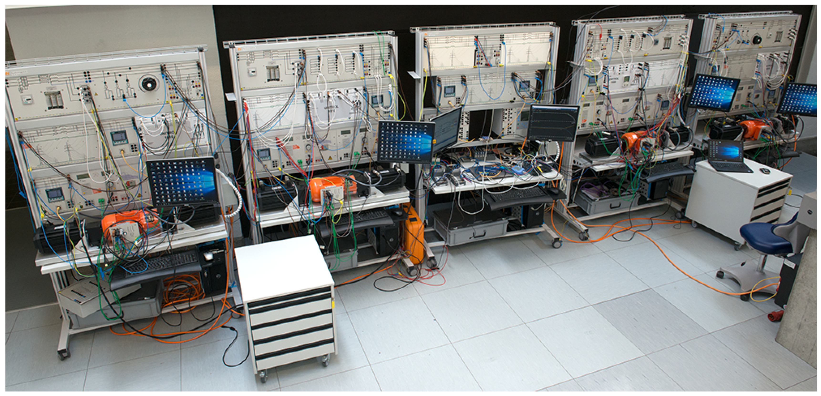
Figure 1.
DHEPS in the REE-LAB of ZHAW.
Figure 1.
DHEPS in the REE-LAB of ZHAW.
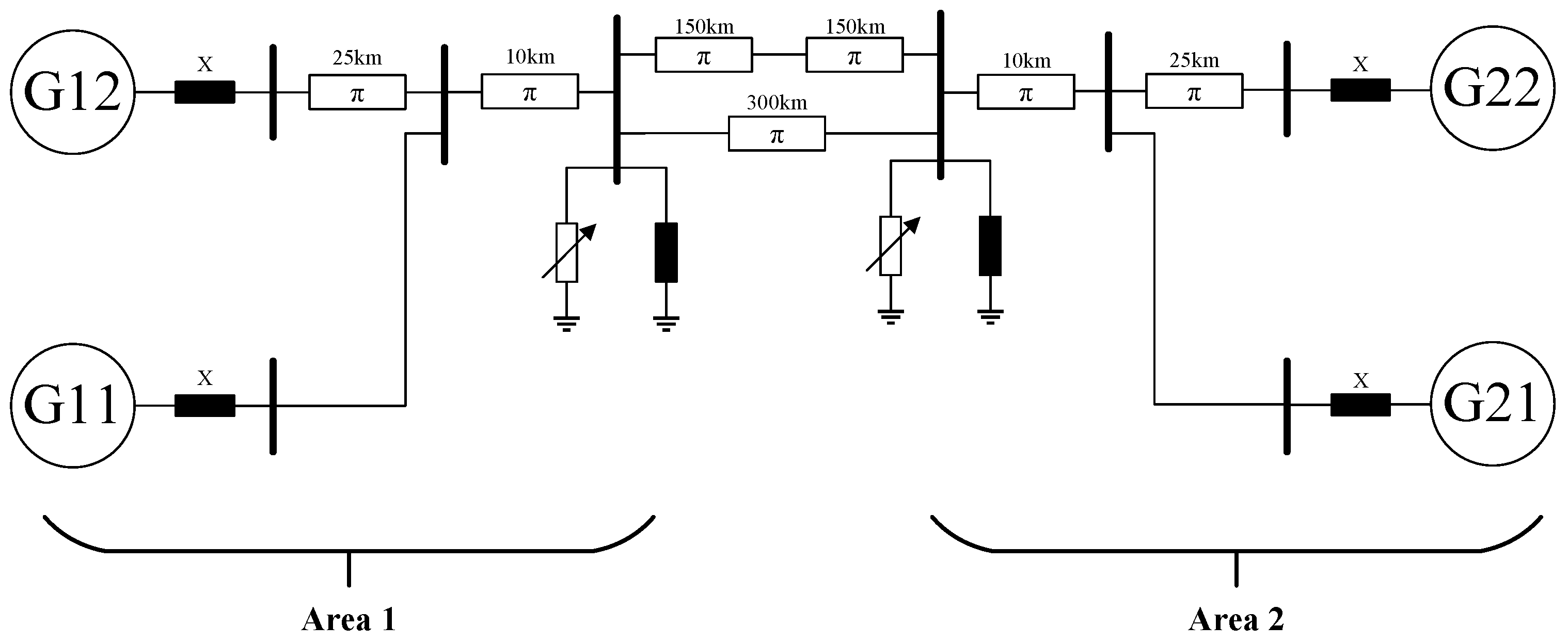
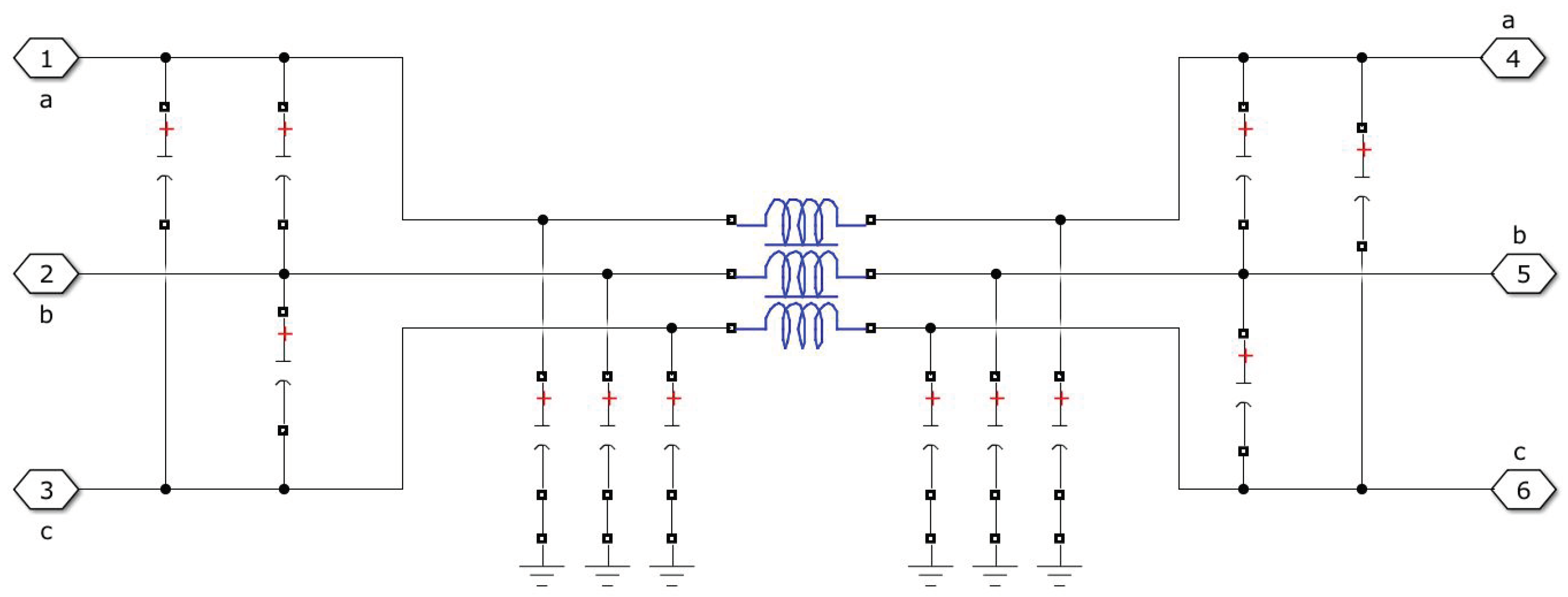
Figure 2.
Single line diagram of the dynamic hardware emulator implemented in the lab according to [
3] with its main components.
Figure 2.
Single line diagram of the dynamic hardware emulator implemented in the lab according to [
3] with its main components.
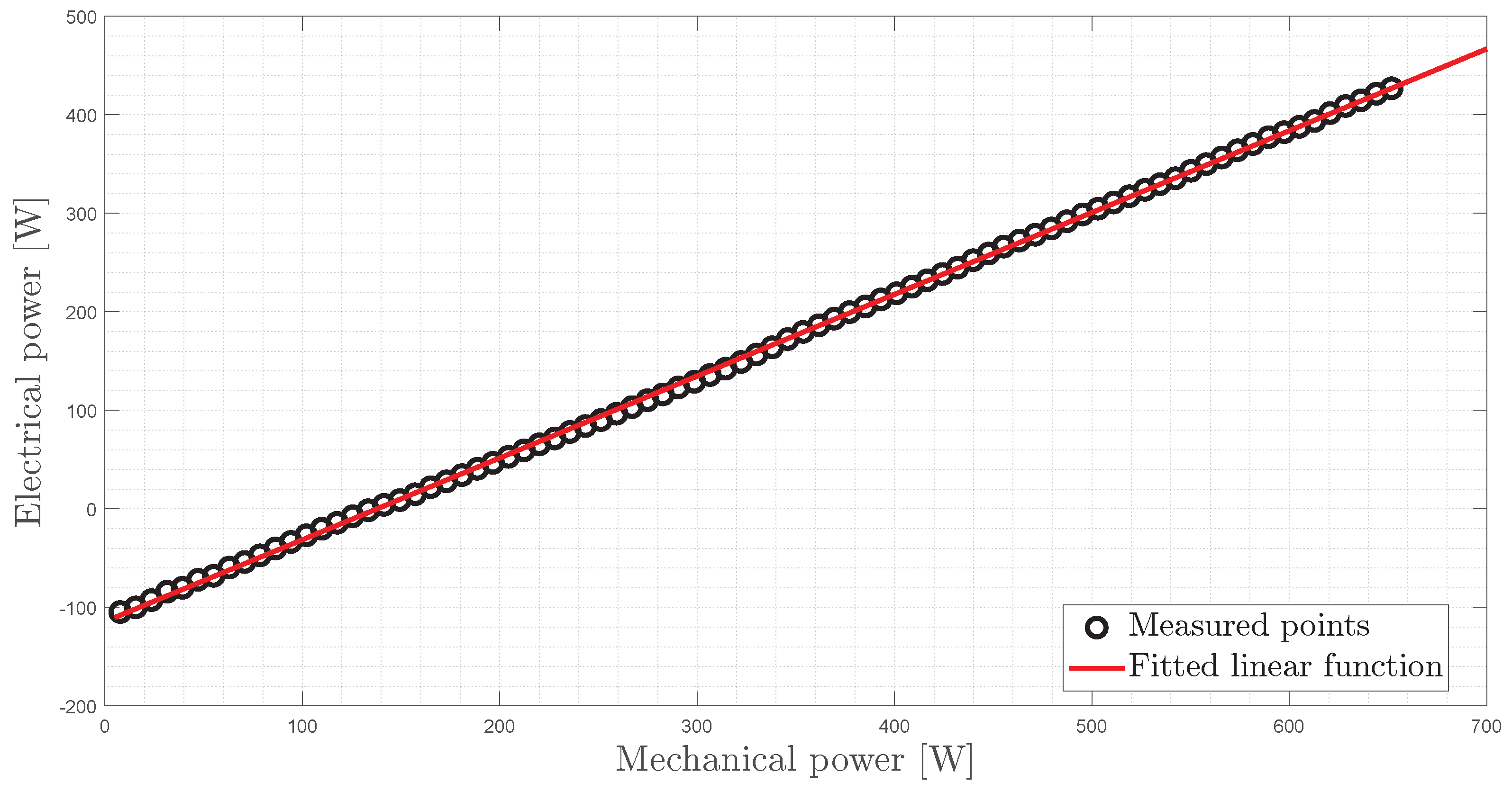
Figure 3.
Measurement (circles) of the experiment and the corresponding fitted linear function.
Figure 3.
Measurement (circles) of the experiment and the corresponding fitted linear function.
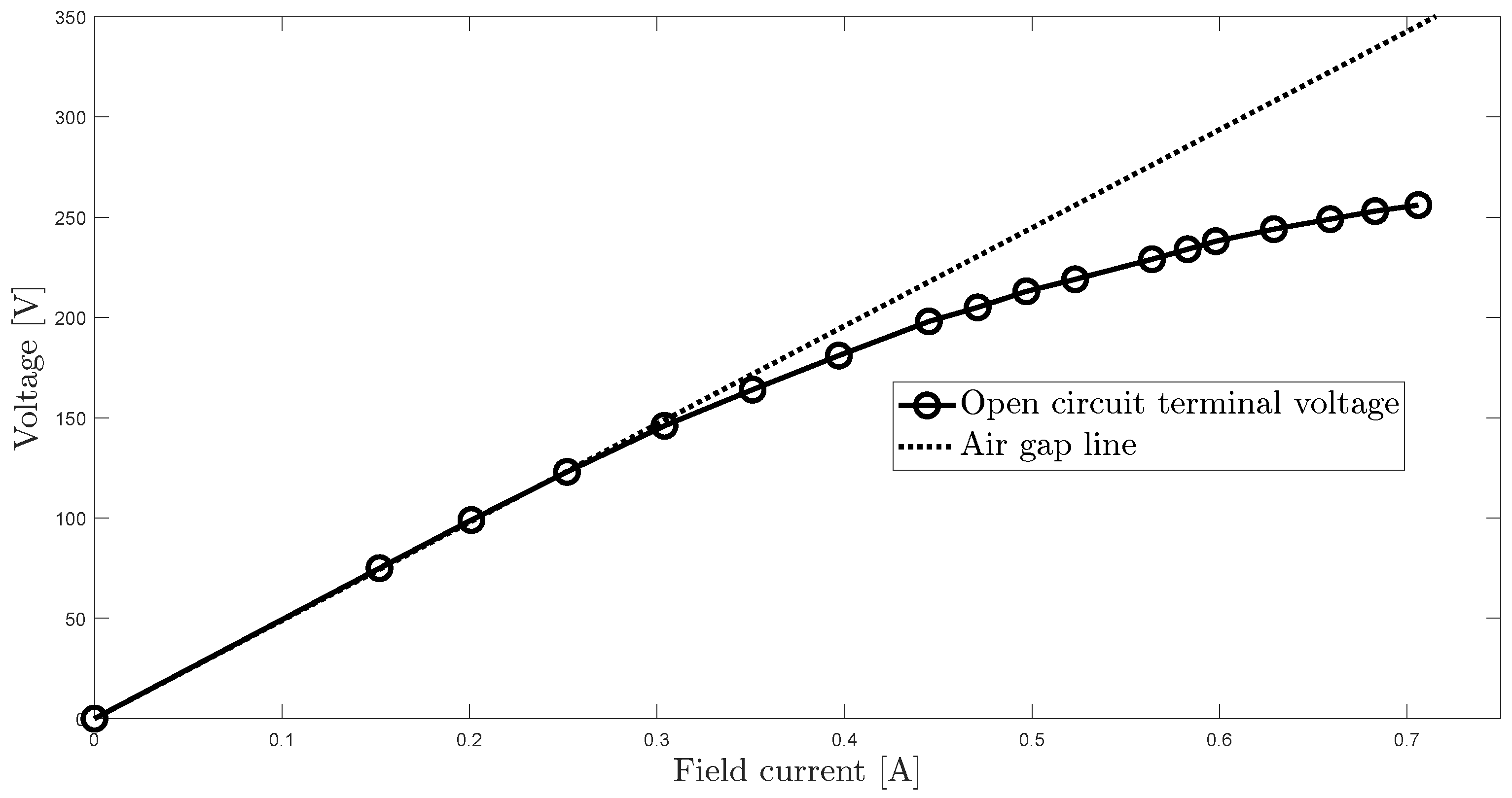
Figure 4.
Open circuit characteristics and air gap line of the synchronous machine under consideration.
Figure 4.
Open circuit characteristics and air gap line of the synchronous machine under consideration.
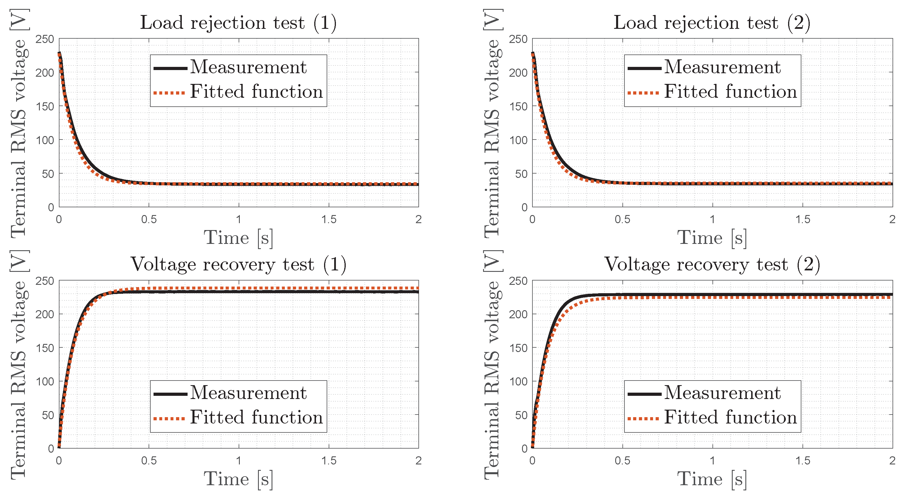
Figure 5.
Top row: Measurement (solid line) and fitted function (dashed red line) of the load rejection test where the same test has been repeated twice. Bottom row: Measurement (solid line) and fitted function (dashed red line) of the voltage recovery test where the same test has been repeated twice.
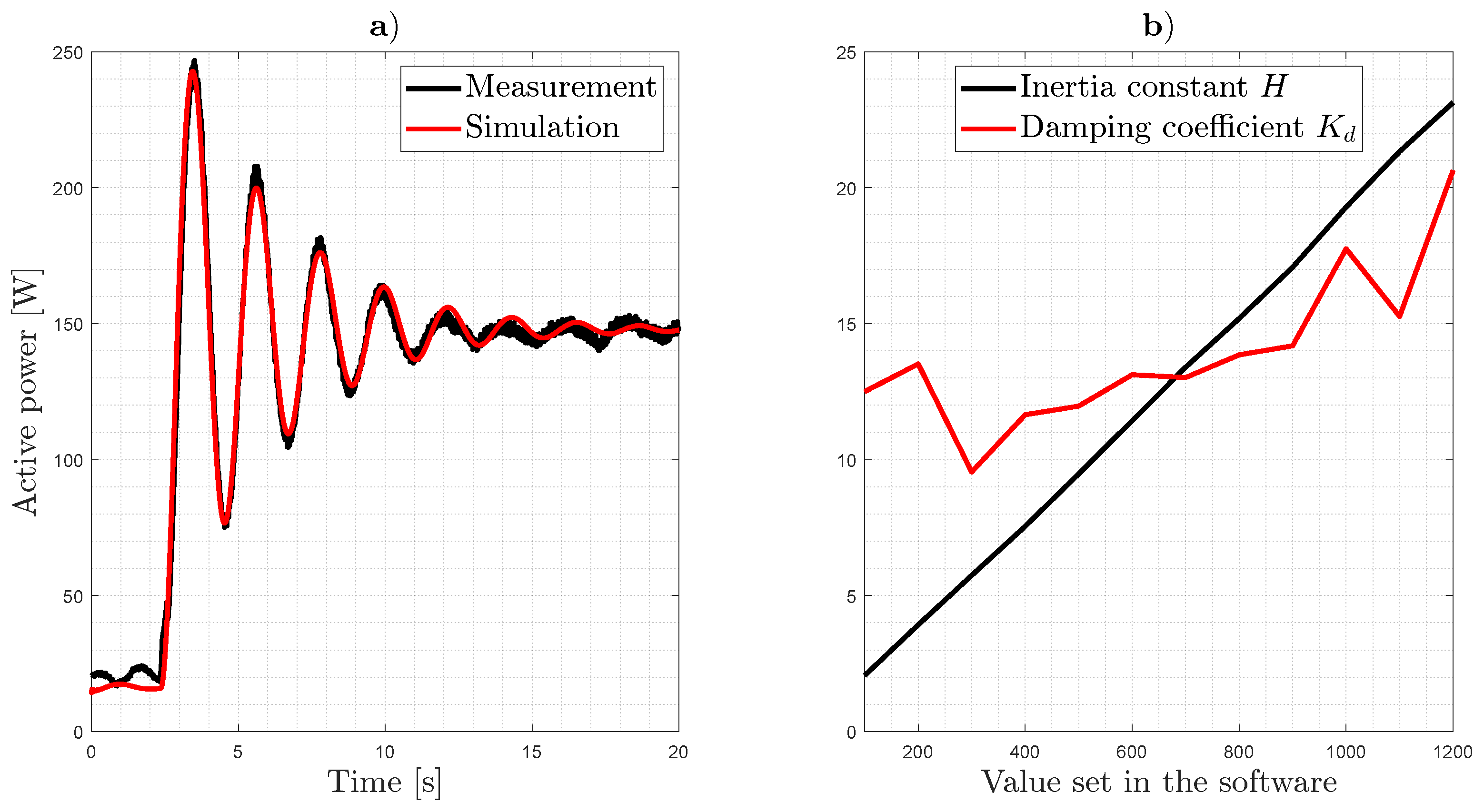
Figure 6.
(a): Active power of the simulation (red) and measured active power (black) after convergence of the parameter estimation tool for a value of 600 defined in the software. (b): Inertia constant H in seconds and damping coefficient in pu depending on the value set in the software.
Figure 6.
(a): Active power of the simulation (red) and measured active power (black) after convergence of the parameter estimation tool for a value of 600 defined in the software. (b): Inertia constant H in seconds and damping coefficient in pu depending on the value set in the software.
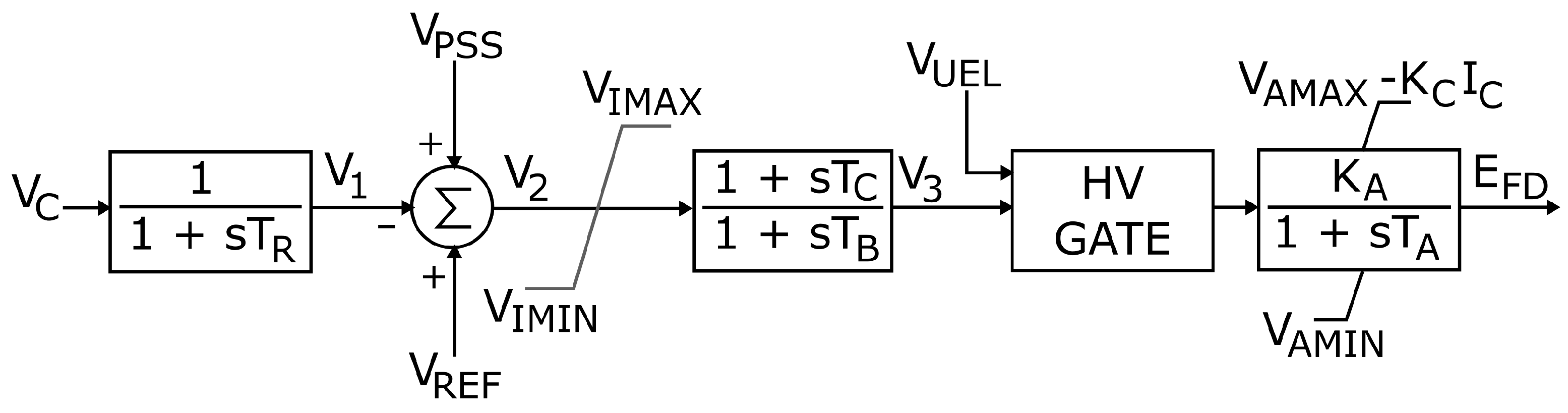
Figure 7.
Block diagram of the excitation system type IEEE AC4A [
21].
Figure 7.
Block diagram of the excitation system type IEEE AC4A [
21].
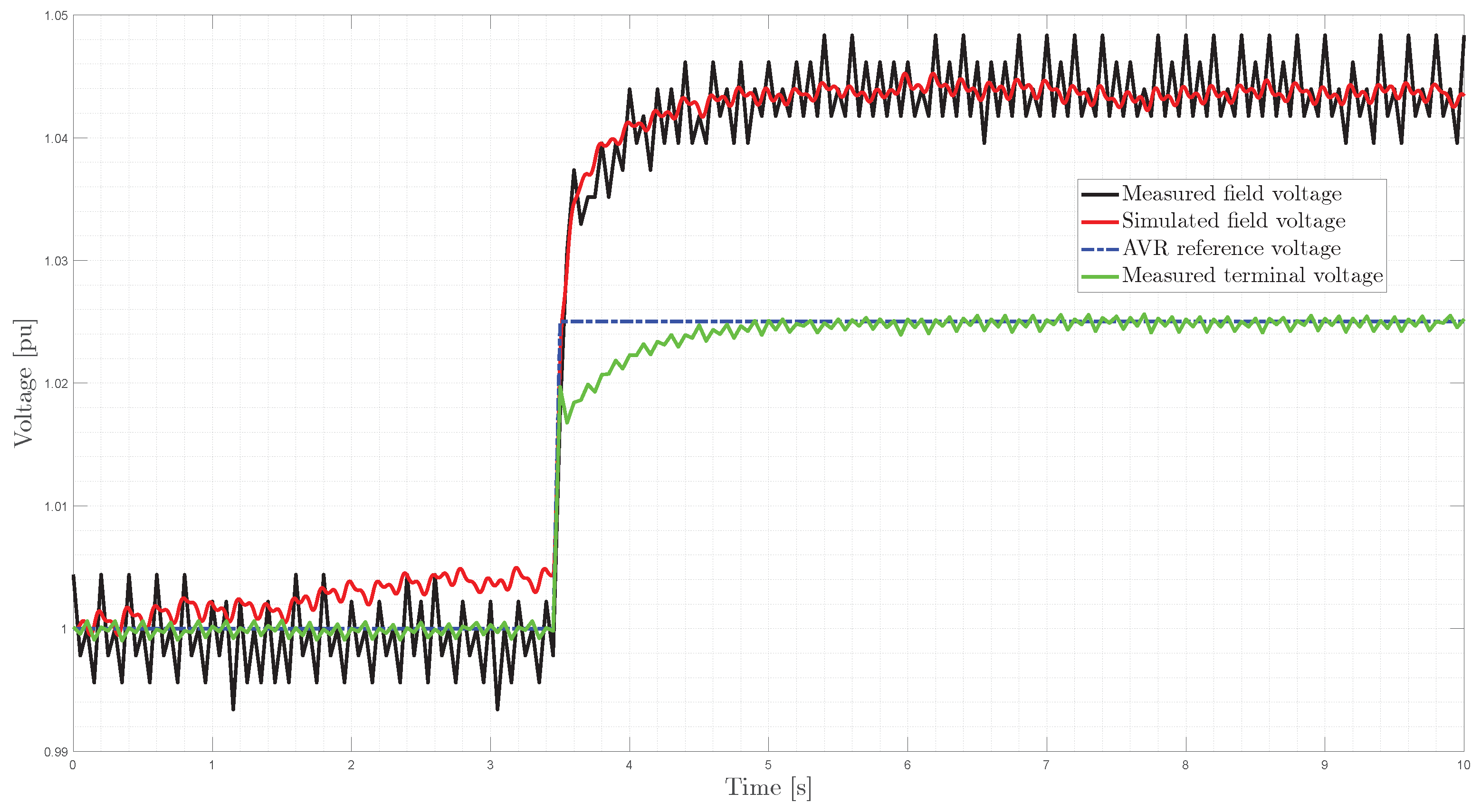
Figure 8.
Final result after identification process where the dashed blue line indicates the step in the reference voltage and the black and red line the measured and simulated field voltage.
Figure 8.
Final result after identification process where the dashed blue line indicates the step in the reference voltage and the black and red line the measured and simulated field voltage.
Figure 9.
Representation of the -type transmission line model used in Simulink.
Figure 9.
Representation of the -type transmission line model used in Simulink.
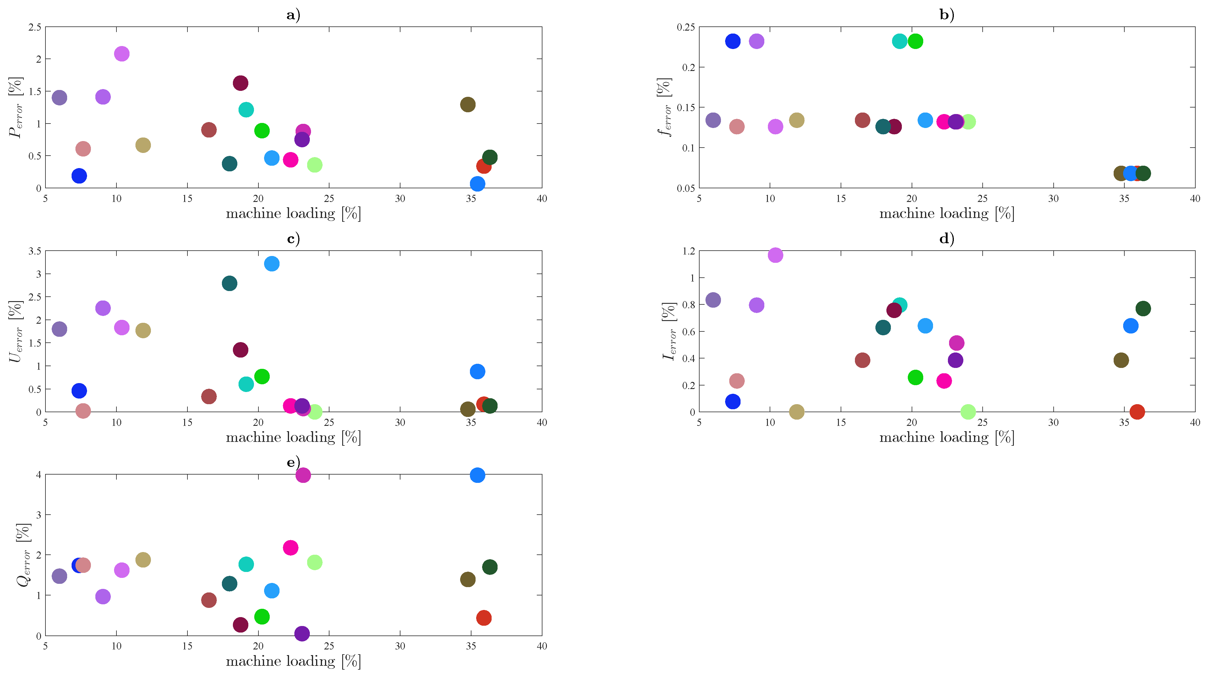
Figure 10.
(a–e) Errors of the measured signals compared to the simulation output in % depending on the loading of the machine.
Figure 10.
(a–e) Errors of the measured signals compared to the simulation output in % depending on the loading of the machine.
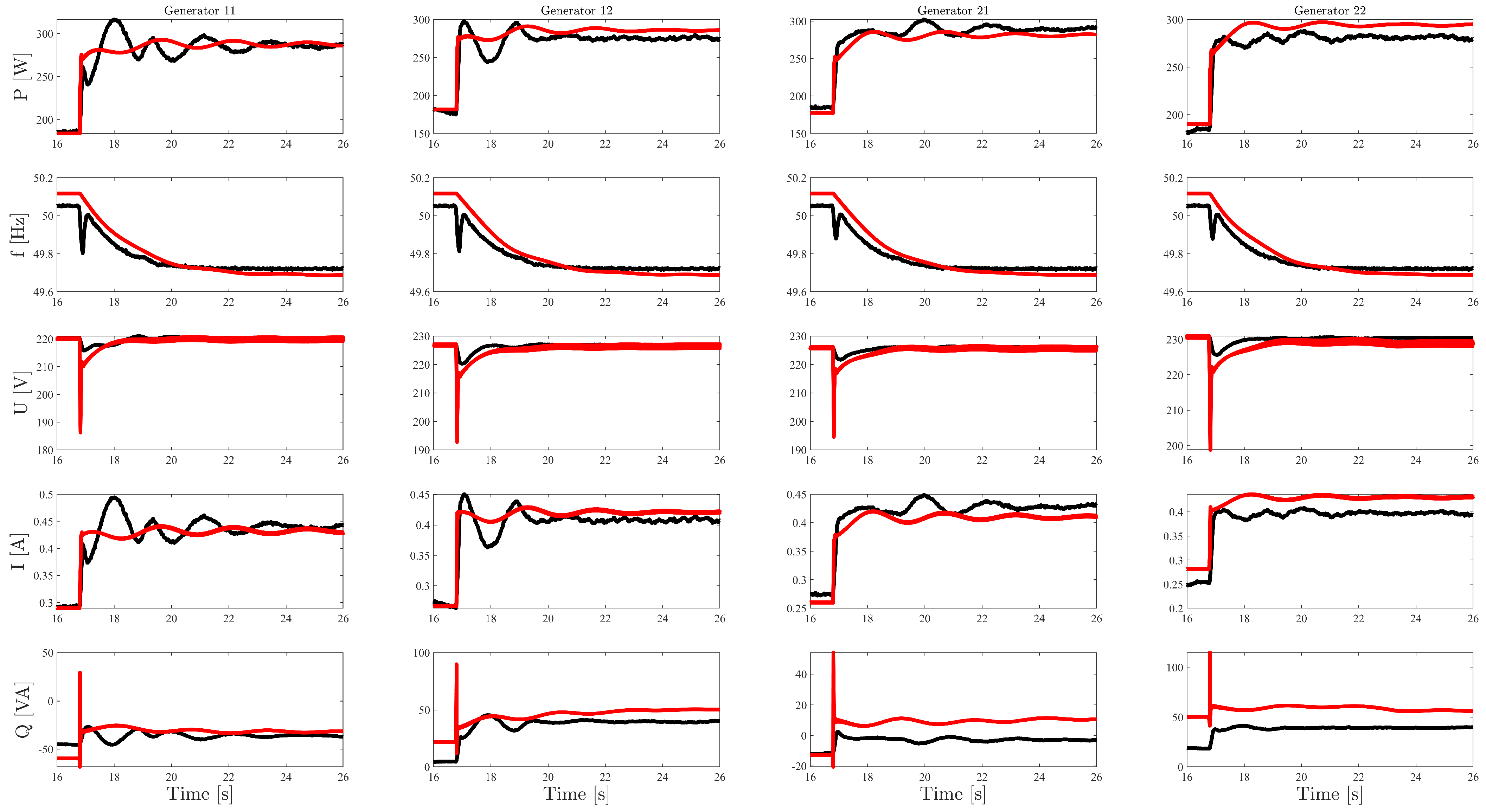
Figure 11.
Measured (black) and simulated (red) signals (active Power P, frequency f, terminal voltage U, phase current I and the reactive power Q) of the the four synchronous machines after the event.
Figure 11.
Measured (black) and simulated (red) signals (active Power P, frequency f, terminal voltage U, phase current I and the reactive power Q) of the the four synchronous machines after the event.
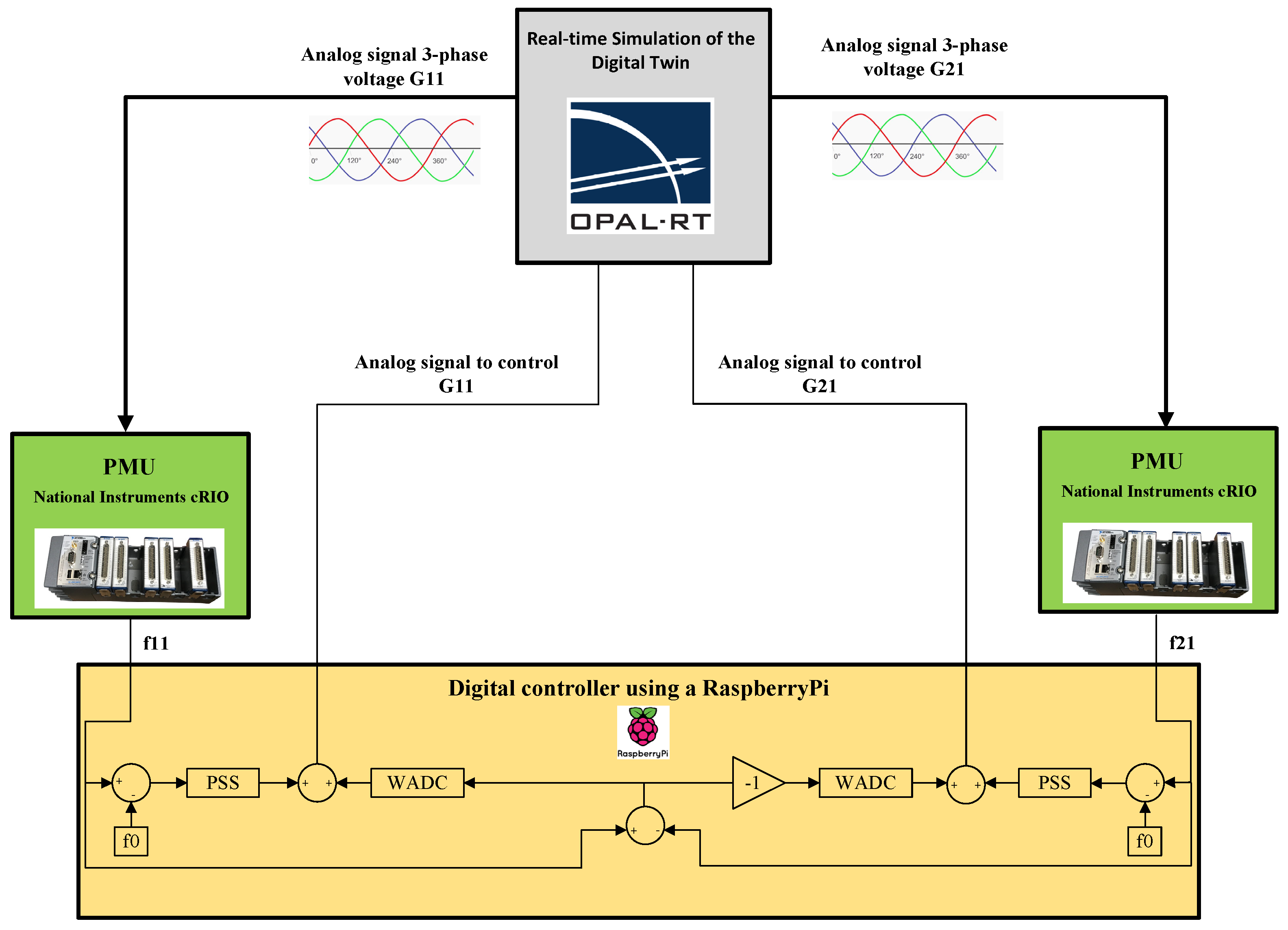
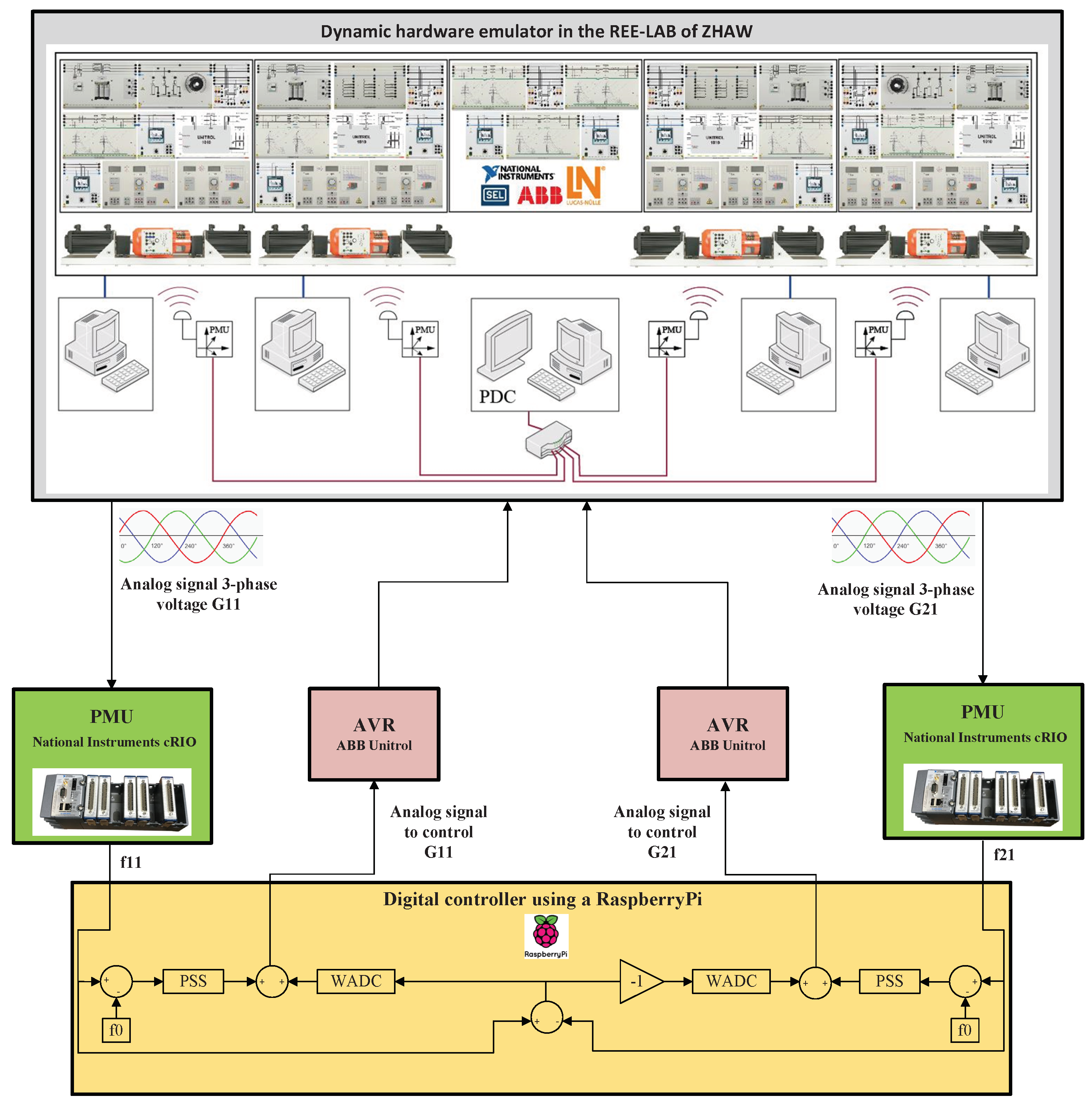
Figure 12.
Schematic drawing of the HIL setup including the real time simulator, PMUs and the digital controller.
Figure 12.
Schematic drawing of the HIL setup including the real time simulator, PMUs and the digital controller.
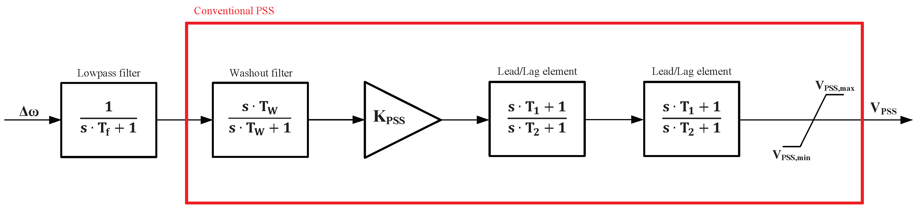
Figure 13.
Conventional PSS (red frame) and the corresponding elements plus a lowpass filter to filter the input signal.
Figure 13.
Conventional PSS (red frame) and the corresponding elements plus a lowpass filter to filter the input signal.
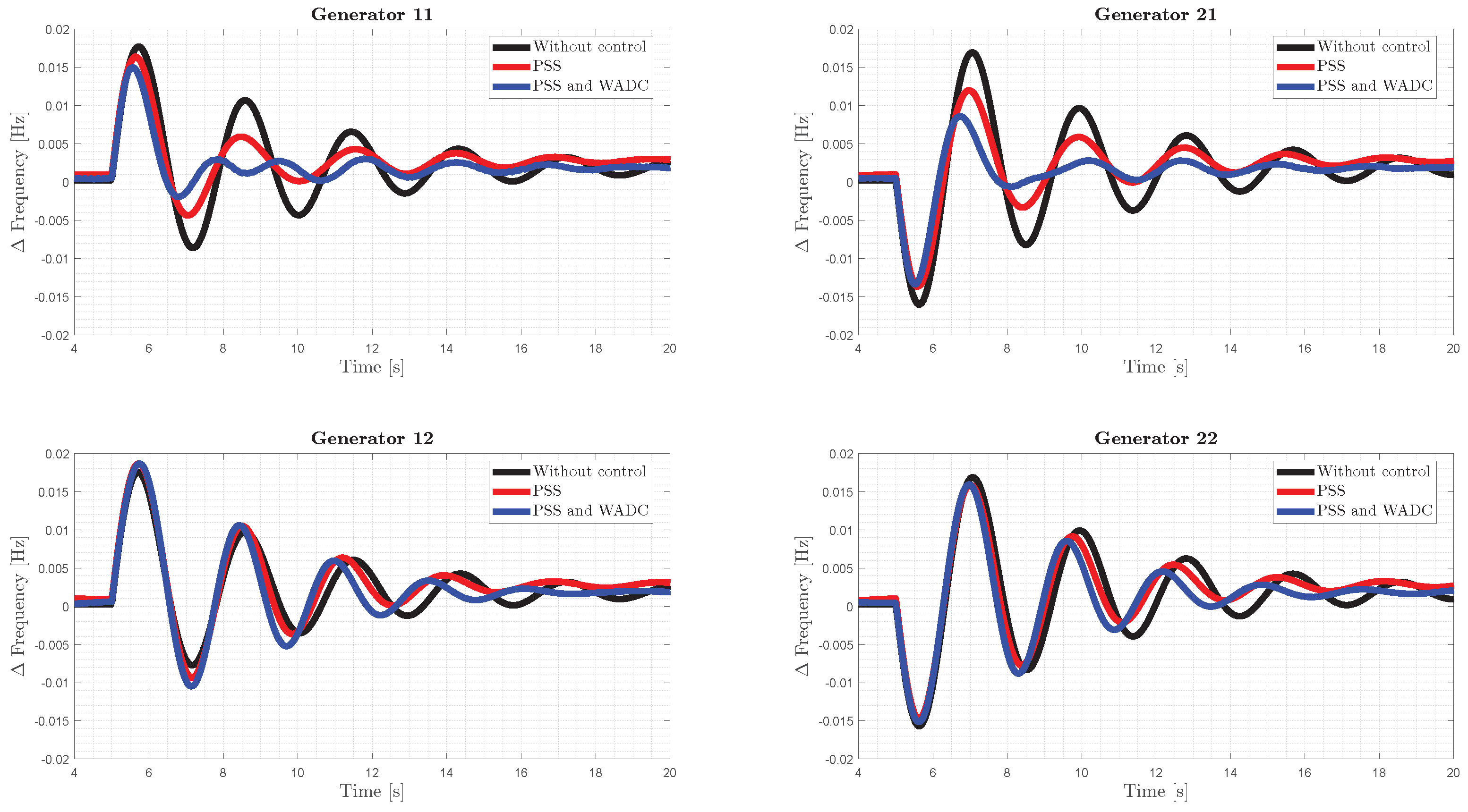
Figure 14.
Comparison of the frequency deviations in the CHIL setup of the three cases (without control, PSS only, PSS and WADC) after applying the same event.
Figure 14.
Comparison of the frequency deviations in the CHIL setup of the three cases (without control, PSS only, PSS and WADC) after applying the same event.
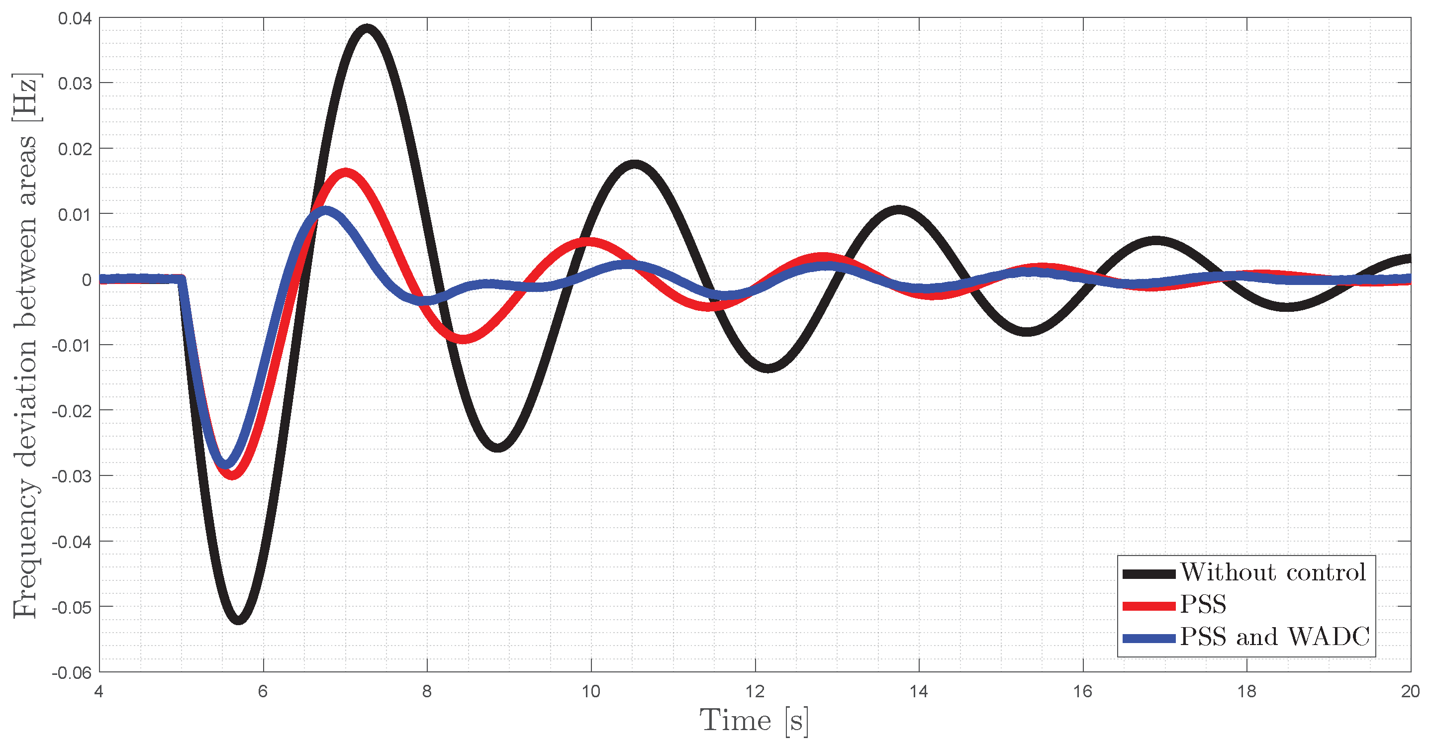
Figure 15.
Frequency deviation between area 1 and area 2 for the three cases (without control, PSS only, PSS and WADC) after the tie line trip within the CHIL setup.
Figure 15.
Frequency deviation between area 1 and area 2 for the three cases (without control, PSS only, PSS and WADC) after the tie line trip within the CHIL setup.
Figure 16.
Schematic drawing of the dynamic hardware emulator setup including the PMUs, the digital controller and the ABB Unitrol.
Figure 16.
Schematic drawing of the dynamic hardware emulator setup including the PMUs, the digital controller and the ABB Unitrol.
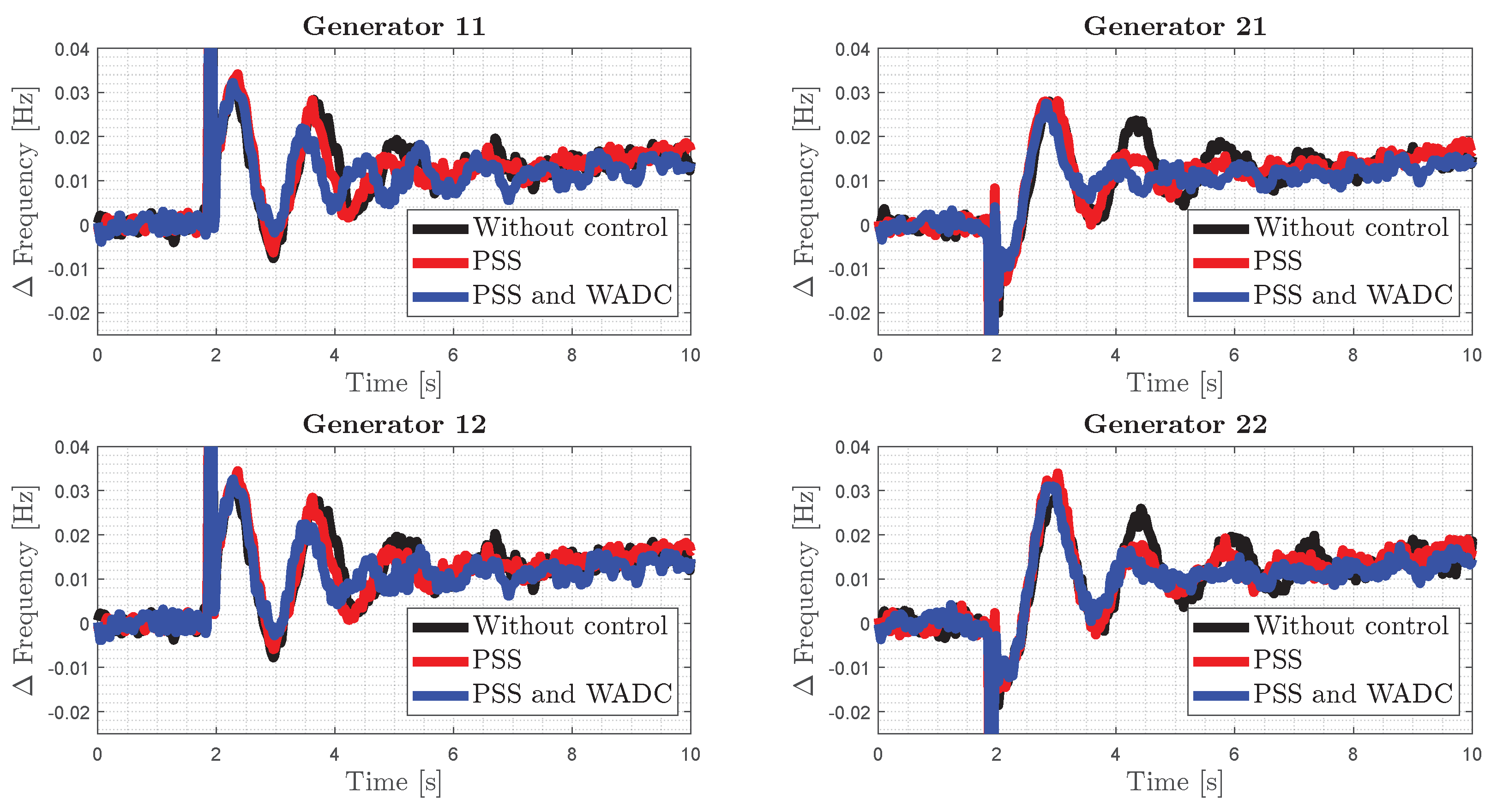
Figure 17.
Frequency deviation with respect to the pre-fault value for the three cases (without control, PSS only, PSS and WADC) after the tie line trip within the setup with the dynamic hardware emulator.
Figure 17.
Frequency deviation with respect to the pre-fault value for the three cases (without control, PSS only, PSS and WADC) after the tie line trip within the setup with the dynamic hardware emulator.
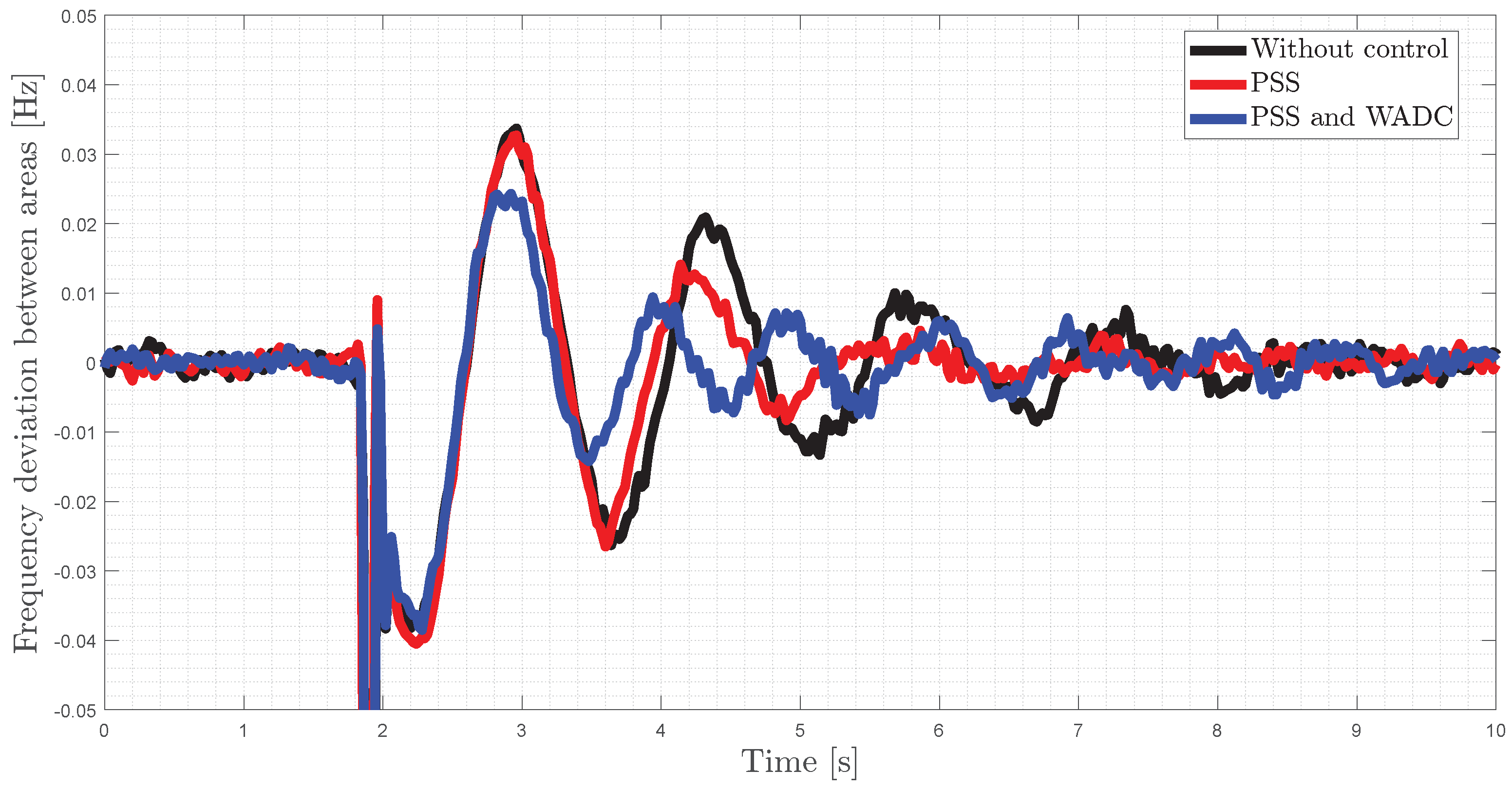
Figure 18.
Frequency deviation between area 1 and area 2 for the three cases (without control, PSS only, PSS and WADC) after the tie line trip within the setup with the dynamic hardware emulator.
Figure 18.
Frequency deviation between area 1 and area 2 for the three cases (without control, PSS only, PSS and WADC) after the tie line trip within the setup with the dynamic hardware emulator.
Table 1.
Ratings of the laboratory synchronous machine according to the plate mounted on the machine.
Table 1.
Ratings of the laboratory synchronous machine according to the plate mounted on the machine.
| Rating | Value |
|---|
| Rated voltage (Y/) | 400/230 V |
| Rated current | 1.5/2.6 A |
| Synchronous speed | 1500 rpm |
| Rated frequency | 50 Hz |
| Rated power | 800 VA |
Table 2.
Generic parameters of a synchronous machine in dq-reference frame.
Table 2.
Generic parameters of a synchronous machine in dq-reference frame.
| d-axis | q-axis |
|---|
| : synchronous reactance | : synchronous reactance |
| : transient reactance | : transient reactance |
| : subtransient reactance | : subtransient reactance |
| : transient open circuit time constant | : transient open circuit time constant |
| : subtransient open circuit time constant | : subtransient open circuit time constant |
Table 3.
Estimated electrical parameters d-axis.
Table 3.
Estimated electrical parameters d-axis.
| Parameter | Value |
|---|
| 322.8 |
| | 3.9 |
| | 0.0798 s |
Table 4.
Estimated parameters of the excitation system IEEE AC4A.
Table 4.
Estimated parameters of the excitation system IEEE AC4A.
| Parameter | Value |
|---|
| 0.01 |
| 32.6876 |
| 0.3408 |
| 0.0347 |
| 310 |
Table 5.
RMSE in % of the signals displayed in
Figure 11.
Table 5.
RMSE in % of the signals displayed in
Figure 11.
| | Generator 11 | Generator 12 | Generator 21 | Generator 22 |
|---|
| RMSE P in %
| 0.96 | 0.56 | 1.00 | 1.28 |
| RMSE f in %
| 0.05 | 0.05 | 0.05 | 0.05 |
| RMSE U in %
| 0.23 | 0.24 | 0.44 | 0.02 |
| RMSE I in %
| 0.35 | 0.31 | 1.21 | 0.65 |
| RMSE Q in %
| 1.61 | 1.07 | 2.99 | 1.00 |
Table 6.
Normalized performance index of the three cases (without control, PSS only, PSS and WADC) for the frequency deviation between the areas within the dynamic hardware emulator setup.
Table 6.
Normalized performance index of the three cases (without control, PSS only, PSS and WADC) for the frequency deviation between the areas within the dynamic hardware emulator setup.
| | Performance Index |
|---|
| Without control | 1 |
| PSS only | 0.86 |
| PSS/WADC | 0.82 |


