Edge Computing Parallel Approach for Efficient Energy Sharing in a Prosumer Community

Abstract

The transition towards more sustainable energy management can be supported by the diffusion of energy communities, i.e., coalitions of prosumers that are willing to exchange the energy produced locally. The optimization of energy management requires the solution of a prosumer problem that can become impractical when the number of users increases. This paper presents a parallel approach, based on an edge computing architecture, which is suitable for large communities. The users are partitioned into groups whose proportions, in terms of producers and consumers, mirror the composition of the whole community. The prosumer problems for the different groups are first solved separately and in parallel by local edge nodes. Then, the solutions are combined by a central entity to redistribute the energy among the groups and minimize the exchange of energy with the external grid. A set of experiments show that the parallel approach, when compared with an approach that solves the optimization problem in a single stage, leads to a notable reduction of computing resources, and becomes feasible in large communities for which the single-stage approach is impossible. Moreover, the achieved solution is close to the optimal solution in terms of energy costs.

1. Introduction

By exploiting the opportunities offered by new technologies, citizens around the world are gaining relevance in the energy sector, through direct actions that aim to build a more sustainable society. This trend is growing, given the reduction of carbon emissions in the electricity sector expected by 2050 [1], it is estimated that 264 million citizens of the European Union will join the energy market as prosumers, generating up to 45% of the total amount of renewable energy. Innovative forms of prosumption (prosumption involves both production and consumption rather than focusing on one or the other) can be implemented in energy communities; that is, coalitions of users who, through voluntary adherence to a contract, collaborate to produce, consume, and manage the energy of one or more local energy plants [2]. Decentralization and localization of energy production are the principles on which an energy community is founded [3].

To address these issues, the European Commission has published a Clean Energy Package: the objective is to offer clean energy to all Europeans through a proposal of an internal market for electricity by revising electricity regulations. The concept of a “local energy community” is defined in Article 16 [4], and it is considered an efficient way to manage energy at the community level. Market participants can profit from advantageous local market prices, and prosumers can generate additional revenue by selling their energy directly to individual consumers [5,6].

The management of energy, and the related costs, can be optimized by solving the prosumer problem, which, given the requirements of users, the availability of energy, and the trend of the energy market aims to determine: (i) the optimal scheduling of loads, (ii) the usage of energy storage systems, and (iii) the exchange of energy among the prosumers of the community. There are numerous approaches to achieving these objectives, mainly based on the solution of a Mixed Integer Linear Programming (MILP) problem, where the objective is the minimization of a cost function (it can be the monetary cost or the total energy consumption), and the constraints are given by the balances of energy on the prosumers and by their requirements. The main limitation of the existing MILP models, for example, those proposed in [7,8,9,10,11,12,13], is that they are not fully scalable. The amount of memory required to solve the prosumer problem increases quadratically with the number of prosumers, since the problem is represented by a matrix in which the rows are the constraints and the columns are the involved variables, and both increase linearly. Moreover, the expected value of the computing time grows as a polynomial function [14], but in the worst case, the computing time increases exponentially, since the optimization of the cost function has NP-hard complexity [15]. Depending on the constraints and requirements—for example, the availability of memory and the time constraints, especially with real-time execution—the solution to the problem can soon become impractical in large communities.

To tackle the scalability issue, in this paper, we present a novel Parallel approach. In a large community, instead of solving a single big optimization problem, the approach divides the users into sub-groups, and the optimization problems are solved for the different groups in parallel. The approach is designed over a smart grid architecture based on the Edge Computing paradigm [16,17,18]. Edge Computing brings the computation towards the edge of the network, and close to the users, offering several advantages, among which are low latency, fast response, and strong location awareness. Edge nodes are used as a gateway between the user smart meters and the control center, enabling the energy community to dynamically acquire the overall electricity usage, adjust the electricity price, provide extra electricity if requested by prosumers, and assist the sharing of energy among the prosumers. As a result, a three-level hierarchy is deployed, in which: (i) each user is equipped with a smart meter that collects data about the user’s energy consumption, (ii) at each group, an edge node, equipped with a smart energy-box, coordinates the users of the group and is able to solve the prosumer problem for these users, and (iii) a control center, or aggregator, coordinates the entire energy community and determines the exchange of energy among the groups.

Each prosumer problem involves a reduced number of users and variables, only those regarding a single group, and therefore a limited amount of memory and a reduced computing time. More in detail, the Parallel approach is organized into a preliminary step and two stages. The preliminary step is devoted to the composition of the sub-groups. We have found that the best strategy is to compose each group so that the fraction of producers and consumers mirrors the overall fractions observed in the whole community. In the first stage, the edge node of each group solves a preliminary prosumer problem and schedules the production, consumption, and usage of storage of the local users. This is conducted in parallel with all other groups. The solution quantifies the amount of energy that needs to be retrieved from the external grid or that results in excess and can be provided to the other groups. In the second stage, the solution is refined with the help of the aggregator, which determines the surplus hours at which the overall amount of energy produced within the community is larger than the energy needs of the consumers. The objective of the second stage is to redistribute the energy among the groups of the community. The prosumer problem is again solved in parallel for each group, and the solution takes into account the availability of the prosumers to acquire the surplus energy computed by the aggregator.

The Parallel approach is applicable to any energy community, properly organized into groups, without any limitation on the number of users. We performed a set of experiments to quantify the costs/revenues achieved when using the Parallel approach, both at the end of the first stage and after the second stage, and the computing time. The experiments were performed for two cases, the first in which the community is composed of groups with similar consumption and production profiles, and the second in which the profiles differ from group to group. We assessed how the cost and execution time are affected when varying the size of the group and the number of users, up to 1000 users. Results show that the Parallel approach leads to large advantages in terms of computing time and amount of needed memory, at the cost of a very small increase in energy costs, compared to the approach that considers all the users in the same MILP problem.

The paper is organized as follows: Section 2 discusses some relevant related works; Section 3 describes the architecture on which the Parallel approach is founded and the algorithm exploited for the solution of the prosumer problem; Section 4 provides the details on the optimization model; Section 5 illustrates the two case studies used to test the Parallel approach; Section 6 reports the results obtained in a wide set of experiments; finally, Section 7 concludes the paper and mentions some avenues for future work.

2. Related Work

The efficient exploitation of prosumer communities, which leverage smart-grids to improve electrical energy production and consumption patterns, requires the adoption of complex involved technologies and innovative energy management frameworks. Currently, in many countries around the globe, various collective self-consumption and energy community initiatives involve hundreds or thousands of members. As an example, the Ewerk Prad Cooperative located in Italy manages 17 renewable energy plants and counts 1350 members, while the Morbegno Electric Company produces electricity through 8 hydroelectric plants and supplies 13,000 users [19].

Energy communities can be classified into three categories, depending on their structure [20]. In centralized communities, a central entity participates in the energy market and controls all the electrical devices [21,22]. The development of this kind of structure is largely limited, due to the need for energy management systems (EMSs) having high computation capabilities and dense communication networks, whose complexity continues to grow as the penetration of renewable generation increases [23,24]. In decentralized communities, each user is equipped with low-performance local controllers that determine the operating conditions of distributed generators and controllable loads, independently from the rest of the community [25,26,27,28]. This approach does not exploit the sharing of energy among the users of a community, thus leading to a poor global solution. To overcome the disadvantages presented by centralized and decentralized approaches, a third model has been proposed, i.e., the hybrid community [29,30]. In the hybrid structure, local controllers perform local energy management and optimization at the user level and inform a central controller of the total amount of energy surplus or deficit. The central controller coordinates the community by ensuring that the energy needs and productions can compensate, thus achieving an efficient global optimal management of energy [31,32]. The EMS is based on low-performance controllers hosted by local users, which are boosted by the computational power of the central controller. The hybrid structure has the advantages of flexibility, high processing power, and low operation costs, and is becoming popular in large energy communities [29,33,34]. A hybrid three-layered architecture is proposed in [35], with an “extreme edge” layer, equipped with sensors, smart meters, and other monitoring devices; a “suburbs” layer, which monitors the power consumption of a specific area and enables the cold spinning reserve; and an energy layer that coordinates the whole system.

In this paper, we propose a hybrid structure, organized on a three-level hierarchy, which exploits the capabilities provided by the Edge Computing technology. In particular, Edge Computing brings the computation toward the edge of the network, and close to the users, thus reducing the latency and the data transmission burden, and improving the location awareness [16,17,18,36].

The majority of the approaches implemented by the EMSs of energy communities are based on the solution of MILP problems. In this context, MILP problems aim to minimize a cost, which can be a monetary cost or the total energy consumption, while addressing a number of constraints defined over real, integer, and binary variables. For example, in [7], the problem of coordinating a community of prosumers that can collaboratively share electricity is modeled as an MILP with coupling constraints. The problem is decomposed and solved using the Lagrangian duality and limited information exchange. In [37], an MILP approach for renewable energy communities is applied to a real energy community test-bed that considers a single group of nine energy community members, and involves distributed photovoltaic systems, energy storage systems, different electricity tariff scenarios, and market signals. In [7], the authors implement a decentralized approach for the coordination of a community with a distributed MILP, and assess it in a realistic community composed of up to 200 householders. In [8], Li et al. present a probabilistic solution for isolated micro-grids using chance constraint programming. The problem is converted into an MILP-based model and solved with a General Algebraic Modeling Language (GAMS) using a CPLEX solver.

A day-ahead scheduling of micro-grid resources, where the objective is to minimize the operational cost and the peak load, is presented in [9]. The proposed MILP model is solved using the CPLEX solver in a mathematical programming language platform. In [10], the authors propose an MILP optimization approach to determine the best allocation and dispatch of distributed energy resources for an energy community, while respecting electrical grid operational constraints. In [12,13], the authors present an optimization model for the energy management in a prosumer community, referred to as Unified model. The Unified model exploits an MILP problem, solved with the Branch and Bound algorithm, which takes into account the energy needs of all the prosumers and optimizes energy sharing at the community level. On the other hand, with the Separated model, proposed in [38,39], each prosumer is modeled separately, while with the Cascade model, discussed in [40], the overall solution is obtained by iterating a number of MILP problems, solved in a sequential fashion.

The main limitation of the mentioned approaches is that an MILP problem is not fully scalable for large communities: an MILP problem is at least as complex as an Integer Linear Programming (ILP) problem that, in turn, is at least as complex as a 0–1 integer program. The last problem is convertible to the SAT optimization problem, whose time complexity is NP-hard [15]. As a consequence of this chain, an MILP problem is also NP-hard and requires EMSs with computational resources and time that can become unacceptable as the size of the problem grows. As explained in detail in [14,41,42], MILP algorithms can be solved in a computing time whose average can be expressed as a polynomial function of the instance size, while the worst-case time complexity (in particular for two common algorithms, the Cutting Plane, and the Branch and Bound) is exponential. Furthermore, the memory increases quadratically. Therefore, the computational burden increases significantly with the scale of the problem and, depending on the number of constraints and on the number of available resources, the time and/or space complexity can make the approach impractical for large communities.

The Parallel approach, presented here, helps to overcome the scalability issue, since the optimization problems of the sub-groups are solved in parallel. This strategy enables a significant reduction of memory and computing time, as shown in Section 6.

3. Architecture and Algorithm of the Parallel Approach

This section describes the Parallel approach, firstly focusing on the architecture, based on the Edge Computing paradigm, then on the algorithm for the solution of the prosumer problem.

3.1. Architecture

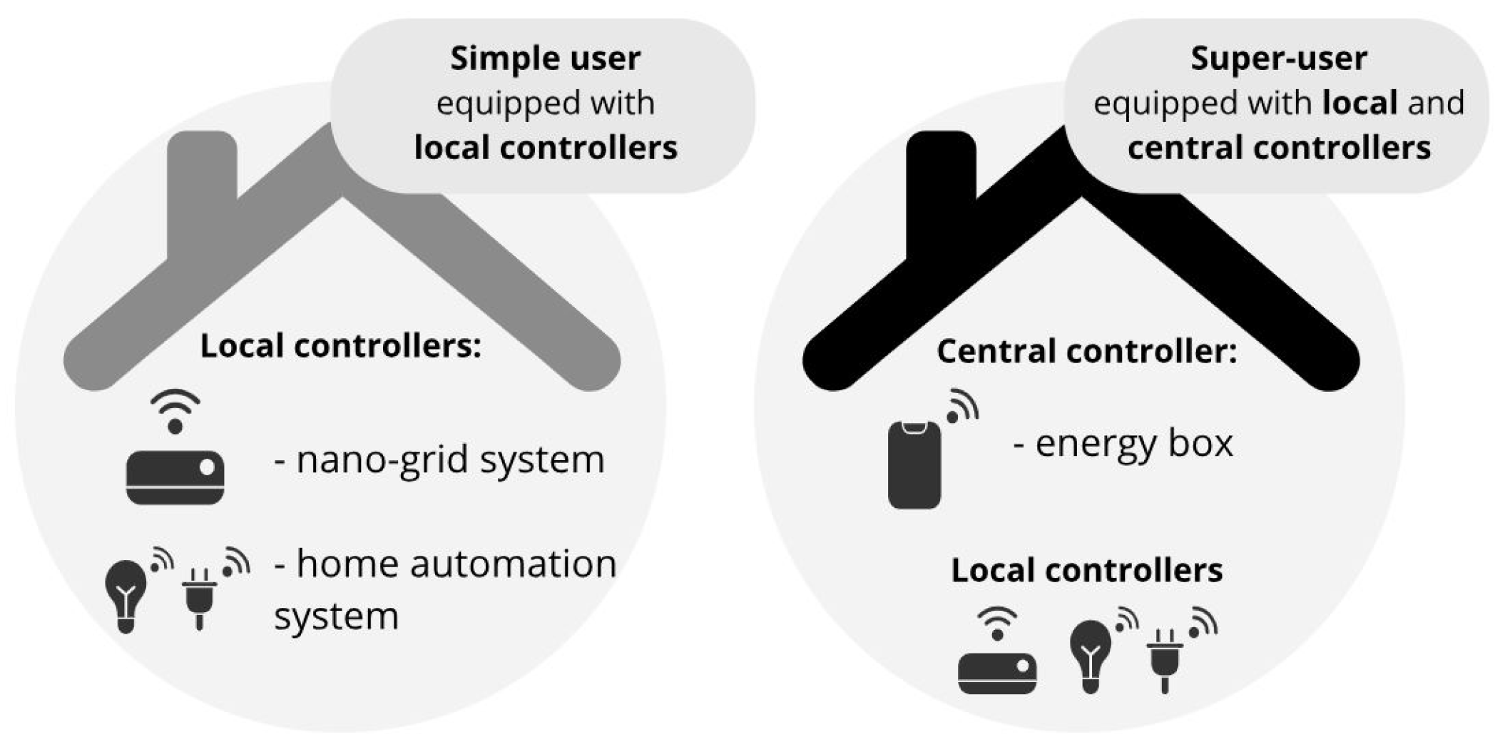
The Parallel approach, presented in this paper, adopts a smart grid infrastructure managed through an Edge Computing architecture. The prosumers are divided into a set of groups acting separately and interacting with a central entity called the aggregator. Each group contains a set of simple users and one super-user. The super-user assumes the role of coordinator of the group and manages the data exchange among the simple users and the aggregator.

Figure 1 shows the equipment of simple users and super-users. Each simple user is equipped with the following local controllers:

• The nano-grid system, which manages and quantifies the energy exchanges among the prosumers, the distribution grid, the local generation plants, and the storage systems;
• The home automation system, which manages the activation/deactivation of the electrical loads, such as the home appliances and the lighting system.

On the other hand, the super-user hosts the energy box, which manages the local controllers of the simple users of the group and the interactions among the group and aggregator.

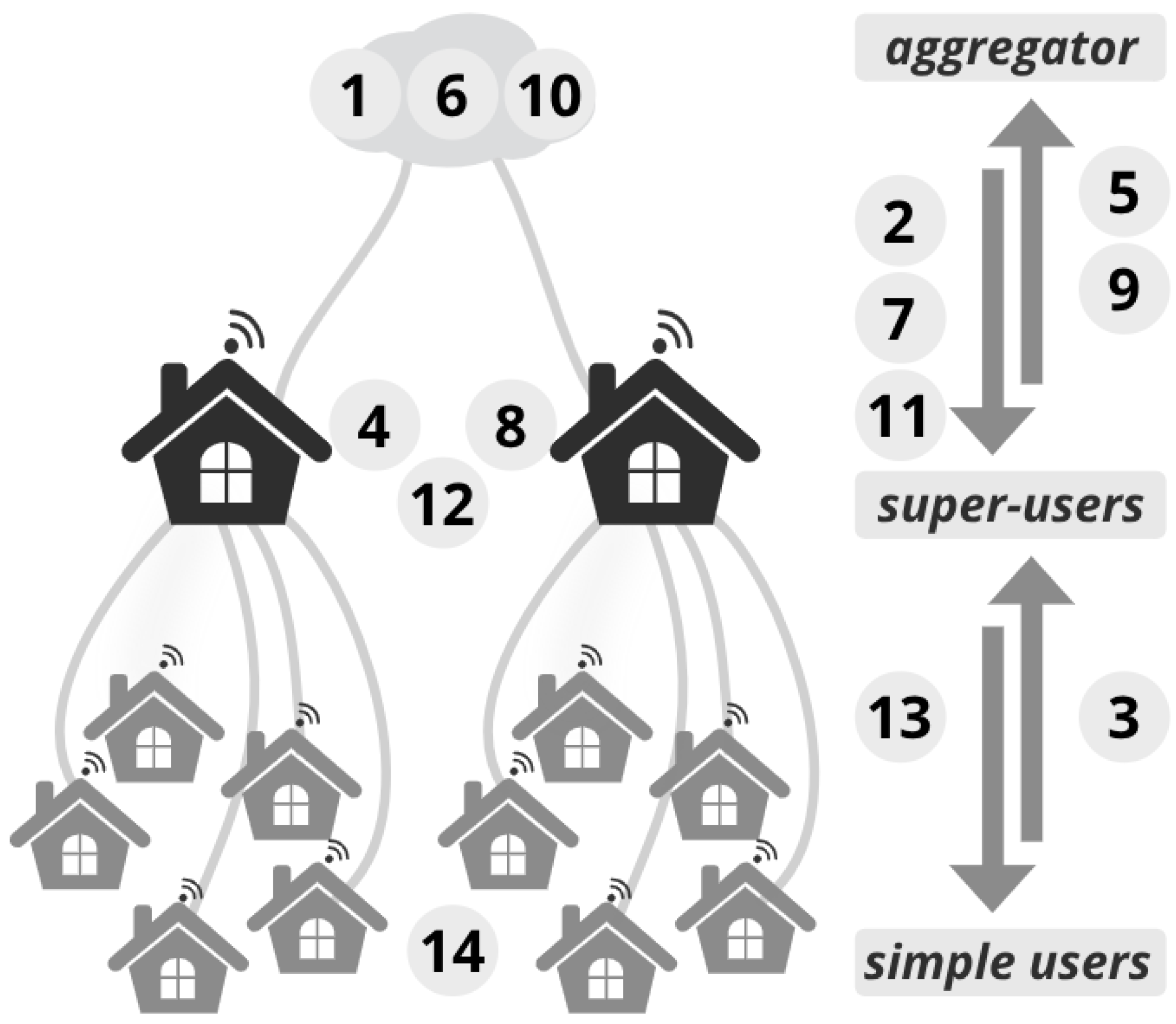
In this context, the aggregator of the community, the super-users, and the simple users take the roles, respectively, of the control center, edge nodes, and smart meters, as shown in Figure 2. In detail:

• The aggregator operates as the control center: it receives, aggregates, and manages the electricity data of the entire community;
• The super-users are used as edge nodes and, through their energy-boxes, collect and aggregate electricity data of the different groups;
• The simple users, through their nano-grids, act as smart meters: they measure local electricity data and send it to the super-user of the local group.

The proposed approach is capable of virtually aggregating prosumers into different groups. The edge nodes use the data collected by the energy meters to monitor and classify the users as producers or consumers, and each edge node is associated with a group of users. The users are chosen according to the criteria defined by the aggregator of the energy community. In general, it is preferable to group users that are physically close to each other, but also remote users can be grouped together, for example, to achieve a given proportion of producers and consumers. Smart grids and intelligent distribution networks ensure the physical connections among the users, and enable the exchange of the energy surplus produced by distributed generation systems.

According to the roles defined before, the energy boxes determine how to manage the local energy systems of the groups, based on the daily information exchanged with the aggregator. In detail, every day the aggregator supplies the following information to the groups:

• The prediction of the energy production and energy consumption, which in turn are based on the weather forecast and on the characteristics and statistics of the generation plants and the electrical loads [43];
• The energy prices, as determined by the energy market (more details are given in Section 5);
• Information about the possible energy surplus: based on the amount of energy produced and consumed inside the community, the aggregator determines if and at which hours a surplus of energy is available, and tries to redistribute this energy to the prosumer groups, as detailed in Section 3.2.

The aggregator computes this information every day for the following day. Based on this information, each energy box determines a working plan for the local nano-grid and home automation system. The objective is to foster the exchange of energy among the prosumers, both belonging to the same group and to different groups, and, in this way, improve energy management and minimize costs.

3.2. Algorithm

In this section, we describe the algorithm exploited by the Parallel approach for the energy management of a large energy community. The aim is to achieve an optimal or suboptimal solution without incurring the complexity issue, both in terms of computing time and amount of memory. Indeed, the solution becomes quicker—because the prosumer problems are executed in parallel on several user groups—and requires less memory, because the amount of memory is determined by the number of users included in a single group.

The Parallel approach is implemented through a preliminary step and two stages, whose chronological flow is described in Figure 3. The example reported in the figure refers to a community of ten users organized into two groups. In the preliminary step, the aggregator divides the energy community into groups (1). We have found that the best strategy is to ensure that in each group the fraction of producers and consumers mirrors the overall proportions observed in the whole community, as will be discussed in Section 6. After the preliminary step, the aggregator delivers to all the super-users the energy prices determined by the energy market and the predictions of energy production and consumption for the next day (2), as computed by the forecast services, which in turn are based on the weather forecast and historical data. Each energy-box receives from the simple users the preferences regarding the scheduling of the electrical loads (3), combine these preferences with the information received from the aggregator, and solves the first stage prosumer problem (4), in order to determine the optimal management of energy for the following day. In this phase, each solution is restricted to the users of the group, and consists of the optimal scheduling concerning the activation/deactivation of the electrical loads, the charging/discharging of the electrical storage systems, the internal energy exchanges between the users of the same group, and the energy exchanges with the outside. At the end of the first stage, all the groups deliver the respective solutions to the aggregator (5), which computes (6) the global energy profile, i.e., the amount of energy produced and consumed for the whole energy community. The aggregator is now able to identify if, and at which hours, the local plants produce more energy than is needed by the prosumers of the community. The aggregator sends this information to the super-users (7), which will use it in the second stage.

The objective of the second stage is to redistribute the energy surplus among the groups. In particular, each energy box solves the second stage prosumer problem, intending to assess: (i) the economical benefit that can derive from the use of the energy surplus with respect to the cost of purchasing the same energy from the grid; and (ii) the benefit that the local producers can obtain by selling the energy surplus within the community rather than to the external grid. Both of these benefits are related to the efficient exchange of energy with the community, as better clarified in Section 5. The second stage is composed of a Request phase and a Grant phase. In the Request phase (8), each prosumer takes into account the amount of surplus energy made available by the other groups and offered at a lower price. The solution to each prosumer problem includes a set of hourly-based energy surplus requests that are collected by the aggregator (9). The aggregator decides which requests can be granted, totally or partially, and which must be rejected (10), and sends the corresponding information to the energy boxes (11). At this point, the energy boxes of the super-users solve the so-called Grant phase optimization model (12). Meanwhile, in the Request phase, each prosumer is free to request any amount of energy surplus that minimizes its objective function; in the Grant phase it can use a fixed amount of energy surplus, that is, the amount granted by the aggregator at each hour. The solution determined at the end of the second stage is sent to the simple users (13), which, in the successive day, will actuate the scheduling using their nano-grids and home automation systems (14). The mathematical models of the first and second stage prosumer problems are detailed in the following Section 4.

4. Optimization Model of the Prosumer Problem

This section provides details on the optimization model that solves the prosumer problems for the different groups of an energy community in a parallel fashion. The optimization problems are modeled as MILP problems, where both binary and real-valued variables are used. The MILP solvers use the Branch and Bound algorithm [44].

In the first stage, the model takes as input the user needs, the energy tariffs, and the energy forecasts related to the following day, and solves the first stage prosumer problem at each group $g\in G$.

In the second stage, the model, starting from the global energy profile resulting from the first stage, identifies the surplus hours and tries to reallocate the surplus energy within the community. The second stage is composed of two phases. In the first phase, named Request phase, the model collects a set of energy surplus requests made by the local users; then, based on the availability of surplus, the model decides which requests can be granted, totally or partially, and which must be rejected. In the second phase, named Grant phase, on the basis of the granted energy surplus requests, the model determines the complete solution of the prosumer problem.

Table 1. Sets of the optimization model.

H	set of the hours of a day
$H^{*}$	set of surplus hours
U	number of users; a single user is denoted with the integer u, $1\le u\le U$
G	number of groups; each group is denoted with the integer g, $1\le g\le G$
$U_g$	set of users that belong to the group g;
$A_u$	set of schedulable loads of user $u\in U_g$
$B_u$	set of non-schedulable loads of user $u\in U_g$

,

Table 2. Variables of the optimization model.

$E_{imp}^{h,u}$	electrical energy imported from the group g at hour $h\in H$ by user $u\in U_g$
$E_{exp}^{h,u}$	electrical energy exported to the group g at hour $h\in H$ by user $u\in U_g$
$E_{impG}^{h,u}$	electrical energy imported from the grid at hour $h\in H$ by user $u\in U_g$
$E_{expG}^{h,u}$	electrical energy exported to the grid at hour $h\in H$ by user $u\in U_g$
$E_{cha}^{h,u}$	electrical energy stored in batteries during hour $h\in H$ by user $u\in U_g$
$E_{dis}^{h,u}$	electrical energy drawn from batteries during hour $h\in H$ by user $u\in U_g$
$y_a^{h,u}$	status of the schedulable load $a\in A_u$ at hour $h\in H$ by user $u\in U_g$ (1 = on; 0 = off)
$z_a^{h,u}$	auxiliary variable set to 1 if the schedulable load $a\in A_u$ is activated at hour
	$h\in H$ by user $u\in U_g$, 0 elsewhere
$E_{req}^{h,u}$	electrical surplus energy requested at hour $h\in H^{*}$ by user $u\in U_g$

and

Table 3. Constants of the optimization model.

${\alpha }_a^u$, ${\beta }_a^u$	start and end time range for scheduling the load $a\in A$ of user $u\in U_g$
${\theta }_a^u$	duration of the working time of the schedulable load $a\in A$ of user $u\in U_g$
$E_a^{h,u}$	rated hourly power of the load $a\in A$ of user $u\in U_g$
$x_b^{h,u}$	consumption forecast for non-schedulable load $b\in B$ at hour $h\in H$
	of user $u\in U_g$
$E_{PV}^{h,u}$	production forecast for PV plants at hour $h\in H$ of user $u\in U_g$
$E_{maxGrid}^u$	maximum operation power that can be imported from the grid
${\eta }_{cha}^u$, ${\eta }_{dis}^u$	charging/discharging efficiency factors of the electrical storage system
	of user $u\in U_g$
$SO{C}_{max}^u$	maximum percentage of the state of charge of the electrical storage system
	of user $u\in U_g$
$SO{C}_{min}^u$	minimum percentage of the state of charge of the electrical storage system
	of user $u\in U_g$
$E_{maxCha}^u$	maximum charging power of the electrical storage system of user $u\in U_g$
$E_{maxDis}^u$	aximum discharging power of the electrical storage system of user $u\in U_g$
$C_{max}^u$	maximum capacity of the electrical storage system of user $u\in U_g$
$E_{STO}^u$	residual energy of the day before stored in the electrical storage system
	of user $u\in U_g$
$c^h$, $p^h$	buying/selling tariffs applied when importing/exporting energy
	inside the community
$c_s^h$	cost to import an electrical $kWh$ of surplus energy at hour $h\in H^{*}$
$PU{N}^h$	buying cost applied when importing energy from the external grid
$P{Z}^h$	selling price applied when exporting energy to the external grid
$E_{expFS}^{h,u}$	electrical energy exported into the grid in the first stage at hour $h\in H^{*}$
	by user $u\in U_g$
$E_{acc}^{h,u}$	amount of energy surplus granted at hour $h\in H^{*}$ to user $u\in U_g$

report, respectively, the sets, variables, and constants used in the optimization model.

4.1. First Stage

The optimization model described in this section is implemented in a parallel fashion at each group $g\in G$ of the community.

The objective function of the optimization model aims to minimize the global energy cost obtained by summing the energy costs (positive values) and the revenues (negative values) of the community users, computed starting from the electrical energy tariffs defined by the daily trend of the energy market (see Section 5).

$$min\sum _{u\in U_g}\sum _{h\in H}(c^h\ast E_{imp}^{h,u}-p^h\ast E_{exp}^{h,u}+PU{N}^h\ast E_{impG}^{h,u}-P{Z}^h\ast E_{expG}^{h,u})$$

(1)

The expression in Equation (1) is defined as the sum for each user $u\in U_g$ of four quantities: the cost incurred by user u at hour h to import energy from the prosumers belong to the same group ($c^h\ast E_{imp}^{h,u}$); the revenue obtained by user u at hour h by selling energy to the users of the same group ($p^h\ast E_{exp}^{h,u}$); the cost incurred by user u at hour h to import energy from the external grid ( $PU{N}^h\ast E_{impG}^{h,u}$); the revenue obtained by user u at hour h by selling energy to the external grid ($P{Z}^h\ast E_{expG}^{h,u}$).

The main constraints of the optimization model are discussed in the following. The temporal granularity for all the quantities is the hour, e.g., the power consumed by the loads as well as the power produced by the plants or exchanged with the storage systems at a given hour (say, 9:00) are assumed to be constant within an hour interval (between 9:00 and 10:00), consequently, the power values expressed as energy/hour, can be considered as an amount of energy. In detail, Equation (2) describes the energy balancing for each user $u\in U_g$ and at each hour $h\in H$:

$$\begin{array}{c}{E}_{imp}^{h,u}+E_{impG}^{h,u}-E_{exp}^{h,u}-E_{expG}^{h,u}+{\eta }_{dis}^u·E_{dis}^{h,u}-\frac{1}{{\eta }_{cha}^u}·E_{cha}^{h,u}-\sum _{a\in A_u}{y}_a^{h,u}·E_a^{h,u}\\ =\sum _{b\in B_u}{x}_b^{h,u}-E_{PV}^{h,u}\forall h\in H,\forall u\in U_g\end{array}$$

(2)

In the balance, the following energy components related to user $u\in U_g$, are considered: the energy supplied by the users of the group g ($E_{imp}^{h,u}$); the energy imported from the grid ($E_{impG}^{h,u}$); the energy supplied to the users of the group g ($E_{exp}^{h,u}$); the energy injected to the grid ($E_{expG}^{h,u}$); the energy supplied by the storage system (${\eta }_{dis}^u·E_{dis}^{h,u}$); the energy charged in the storage system ($\frac{1}{{\eta }_{cha}^u}·E_{cha}^{h,u}$); the sum of the energy amount consumed by the schedulable loads $a\in A_u$ ($y_a^{h,u}·E_a^u$) computed as the products of the variables $y_a^{h,u}$ and the rated powers $E_a^u$; the sum of the forecast energy quantities consumed by non-schedulable loads $b\in B_u$ ($x_b^{h,u}$); and the forecast energy produced by the local PV generators ($E_{PV}^{h,u}$).

Equation (3) balances the energy flows exchanged among users of the group g:

$$\sum _{u\in U_g}(E_{imp}^{h,u}-E_{exp}^{h,u})=0\forall h\in H$$

(3)

The inequality (4) forces the total amount of imported energy, i.e., from the group ($E_{imp}^{h,u}$) or from the external grid ($E_{impG}^{h,u}$), not to exceed the maximum operation power of the Point Of Delivery, $E_{maxGrid}^u$.

$$E_{imp}^{h,u}+E_{impG}^{h,u}\le E_{maxGrid}^u\forall h\in H,\forall u\in U_g$$

(4)

Equations (5) and (6) force the activation of load a to occur at a single hour $h\in [{\alpha }_a^u,{\beta }_a^u-{\theta }_a^u+1]$. The upper bound of the latter interval is set to ${\beta }_a^u-{\theta }_a^u+1$, instead of ${\beta }_a^u$, to ensure that the working time of the load a ends before ${\beta }_a^u$.

$$\sum _{h={\alpha }_a^u}^{{\beta }_a^u-{\theta }_a^u+1}{z}_a^{h,u}=1\forall a\in A_u,\forall u\in U_g$$

(5)

$$z_a^{h,u}=0\forall h\in H\backslash [{\alpha }_a,{\beta }_a-{\theta }_a+1],\forall a\in A_u,\forall u\in U_g$$

(6)

Equation (7) ensures that the load a of user u is activated exactly for ${\theta }_a^u$ hours inside the $[{\alpha }_a^u,{\beta }_a^u]$ preference interval.

$$\sum _{h={\alpha }_a^u}^{{\beta }_a^u}{y}_a^{h,u}={\theta }_a^u\forall a\in A_u,\forall u\in U_g$$

(7)

Inequality (8) forces every schedulable load $a\in A_u$ to operate during its working time, without interruptions. Enabling or disabling this facility depends on the user’s request.

$$y_a^{h,u}\ge z_a^{h,u},y_a^{h+1,u}\ge z_a^{h,u},\dots ,y_a^{h+{\theta }_a-1,u}\ge z_a^{h,u}\forall h\in [{\alpha }_a,{\beta }_a],\forall a\in A_u,\forall u\in U_g$$

(8)

with reference to users that hold electric storage systems, inequalities (9) and (10) express the fact that the total stored energy at each hour $h\in H$ is within the allowed minimum and maximum states of charge ($SO{C}_{min}^u$ and $SO{C}_{max}^u$). As introduced, $E_{cha}^{i,u}$ is the stored energy and $E_{dis}^{i,u}$ is the energy supplied by the storage system of user u during the hour h.

$$E_{STO}^u+\sum _{i=0}^h{E}_{cha}^{i,u}-\sum _{i=0}^h{E}_{dis}^{i,u}\ge SO{C}_{min}^u\ast C_{max}^u\forall h\in H,\forall u\in U_g$$

(9)

$$E_{STO}^u+\sum _{i=0}^h{E}_{cha}^{i,u}-\sum _{i=0}^h{E}_{dis}^{i,u}\le SO{C}_{max}^u\ast C_{max}^u\forall h\in H,\forall u\in U_g$$

(10)

The constraints related to the maximum amounts of energy drawn and stored by the electrical storage systems are expressed by inequalities (11) and (12):

$$0\le E_{cha}^{h,u}\le E_{maxCha}^u\forall h\in H,\forall u\in U_g$$

(11)

$$0\le E_{dis}^{h,u}\le E_{maxDis}^u\forall h\in H,\forall u\in U_g$$

(12)

Inequalities (13) and (14) force the hourly energy exported by user u to the group ($E_{exp}^{h,u}$) and to the grid ($E_{expG}^{h,u}$) to be positive values:

$$0\le E_{exp}^{h,u}\forall h\in H,\forall u\in U_g$$

(13)

$$0\le E_{expG}^{h,u}\forall h\in H,\forall u\in U_g$$

(14)

Inequalities (15) and (16) force the hourly energy imported by user u from the group ($E_{imp}^{h,u}$) and from the grid ($E_{impG}^{h,u}$) to be positive values, lower than or equal to the maximum operation power ($E_{maxGrid}^u$):

$$0\le E_{imp}^{h,u}\le E_{maxGrid}^u\forall h\in H,\forall u\in U_g$$

(15)

$$0\le E_{impG}^{h,u}\le E_{maxGrid}^u\forall h\in H,\forall u\in U_g$$

(16)

4.2. Second Stage

This section describes the second stage of the parallel optimization model, composed of the Request phase and the Grant phase.

4.2.1. Request Phase

The model for the request phase of the second stage uses the same variables as the first stage model plus another set of variables, $E_{req}^h,u$, which are the amounts of energy surplus that the prosumer will request. The same constraints and upper/lower bounds as the first stage model are also adopted, with the differences and the additions that are specified in the following.

The objective function—see expression (1)—and the electrical balance constraint—see Equation (2)—of the first stage model are substituted with the expression (1) and the Equation (18), in which the new variables $E_{req}^h$ are now considered.

$$min\sum _{u\in U_g}\sum _{h\in H}(c_s^h\ast E_{req}^{h,u}+c^h\ast E_{imp}^{h,u}-p^h\ast E_{exp}^{h,u}+PU{N}^h\ast E_{impG}^{h,u}-P{Z}^h\ast E_{expG}^{h,u})$$

(17)

$$\begin{array}{c}{E}_{req}^{h,u}+E_{imp}^{h,u}+E_{impG}^{h,u}-E_{exp}^{h,u}-E_{expG}^{h,u}+{\eta }_{dis}^u·E_{dis}^{h,u}-\frac{1}{{\eta }_{cha}^u}·E_{cha}^{h,u}-\sum _{a\in A_u}{y}_a^{h,u}·E_a^{h,u}\\ =\sum _{b\in B_u}{x}_b^{h,u}-E_{PV}^{h,u}\forall h\in H,\forall u\in U_g\end{array}$$

(18)

The hour-by-hour electrical energy exported with the grid, as resulting from the solution to the first stage model, is introduced in the request phase of the second stage model as constants $E_{expFS}^h$. Indeed, if the amount of exchanged energy were modified at the second stage, the surplus energy could be no longer available, thus making the execution of the second stage not consistent with the solution to the first stage. Therefore, the amount of energy exported at the normal price during the surplus hours by each prosumer in the second stage must be equal to the corresponding amount of the first stage, which is guaranteed by Equation (19).

$$E_{exp}^{h,u}=E_{expFS}^{h,u}\forall h\in H^{*},\forall u\in U_g$$

(19)

Inequalities (20)–(22) determine the admissible range of values for $E_{req}^h$. In particular, inequality (20) substitutes the analogous inequality in the first stage model, i.e., inequality (4). Expressions (21) and (22) specify that $E_{req}^h$ can be greater than 0 only in the surplus hours, while in the remaining hours, it is equal to zero.

$$E_{req}^{h,u}+E_{imp}^{h,u}+E_{impG}^{h,u}\le E_{maxGrid}^u\forall h\in H,\forall u\in U_g$$

(20)

$$E_{req}^{h,u}\ge 0\forall h\in H,\forall u\in U_g$$

(21)

$$E_{req}^{h,u}=0\forall h\in H\backslash H^{*},\forall u\in U_g$$

(22)

4.2.2. Grant Phase

The model for the grant phase uses the same variables, constants, and constraints as the first-stage model, with the differences specified in the following. The quantities $c_s^h$, $H^{*}$, $E_{expFS}^h$ have the same meaning as in the request phase. New constants $E_{acc}^h$ are introduced, which represent the amount of energy surplus requested by the prosumer and granted by the aggregator.

The objective function, electric balance constraint, and the constraint on the maximum amount of energy that can be imported from the grid are modified accordingly, see expression (23), Equation (24), and inequality (25).

$$min\sum _{u\in U_g}\sum _{h\in H}(c_s^h\ast E_{acc}^{h,u}+c^h\ast E_{imp}^{h,u}-p^h\ast E_{exp}^{h,u}+PU{N}^h\ast E_{impG}^{h,u}-P{Z}^h\ast E_{expG}^{h,u})$$

(23)

$$\begin{array}{c}{E}_{acc}^{h,u}+E_{imp}^{h,u}+E_{impG}^{h,u}-E_{exp}^{h,u}-E_{expG}^{h,u}+{\eta }_{dis}^u·E_{dis}^{h,u}-\frac{1}{{\eta }_{cha}^u}·E_{cha}^{h,u}-\sum _{a\in A_u}{y}_a^{h,u}·E_a^{h,u}\\ =\sum _{b\in B_u}{x}_b^{h,u}-E_{PV}^{h,u}\forall h\in H,\forall u\in U_g\end{array}$$

(24)

$$E_{acc}^{h,u}+E_{imp}^{h,u}+E_{impG}^{h,u}\le E_{maxGrid}^u\forall h\in H,\forall u\in U_g$$

(25)

Similar to what was said for the request phase, in the grant phase, the amount of energy exported to the grid during the surplus hours is set to be equal to the amount computed after the first stage, see Equation (19).

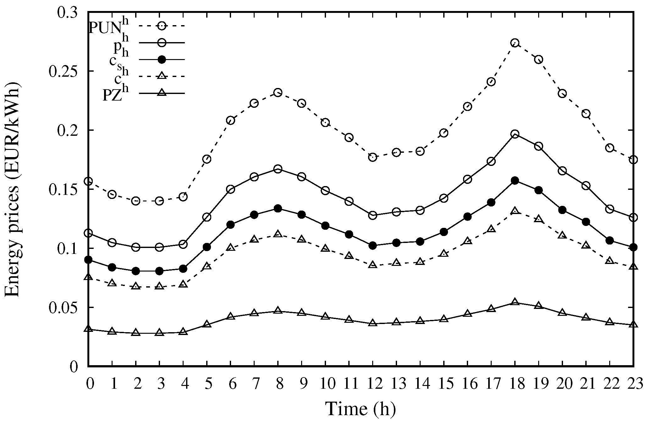
5. Energy Tariffs and Case Studies

The prosumers obtain benefits to join an energy community for two main reasons: (i) the community, through the aggregator, can negotiate directly with the energy provider that applies wholesaler energy prices; (ii) the energy exchange inside the community and between the community and the energy provider can be optimized. The tariffs of electrical energy are determined daily by the energy market. In our scenario, the Italian energy market defines the wholesaler energy prices: the zone price ($P{Z}^h$) and the single national price ($PU{N}^h$), which correspond, respectively, to the selling price and the basic buying cost applied at hour h when importing/exporting energy from/to the external grid. Conversely, the selling price and the buying cost applied to the exchange of energy inside a community are denoted, respectively, by $c^h$ and $p^h$. The users are encouraged to share energy among them if it holds that:

$$PU{N}^h\ge c^h\ge p^h\ge P{Z}^h$$

(26)

As discussed in Section 3.2, in the second stage the aggregator, starting from the solutions of the prosumer problems of the first stage, determines the surplus hours, i.e., the hours at which the energy produced by the whole community exceeds the overall energy demand. The goal of the second stage is to redistribute this energy surplus to the prosumers. To this end, the aggregator puts this energy surplus on sale at a price $c_s^h$, which is more convenient than the purchase prices reserved at the first stage, i.e., $PU{N}^h$ and $c^h$. This price is the same for all the prosumers of the community.

The price $c_s^h$ must be greater than $P{Z}^h$, i.e., the price at which the users sell energy to the grid, otherwise it would be more convenient for the users to sell the energy surplus to the grid rather than distributing it within the community, and there would be no benefit for the whole community. Using these considerations, the inequalities (26) are updated by including the price $c_s^h$, which leads to the inequalities:

$$PU{N}^h\ge c^h\ge \{c_s^h,p^h\}\ge P{Z}^h$$

(27)

The curly brackets in expression (27) indicate that there is no particular order relationship between the values of $c_s^h$ and $p^h$.

To evaluate the performance of the Parallel approach, a set of simulation experiments has been carried out. The experiments were performed to determine the optimal schedule for 20 February 2021. The national selling and buying energy prices for the considered day, $P{Z}^h$ and $PU{N}^h$, were retrieved from the GME, the Italian energy market manager (http://www.mercatoelettrico.org, accessed on 23 May 2022). The prices $c^h$, $p^h$, and $c_s^h$ were established to be compliant to the inequalities (27). Figure 4 shows the trends of these prices and costs for the mentioned day.

In this paper, we present the results achieved when the percentage of prosumers, i.e., of users that are both consumers and producers, is set to 40%, while the remaining 60% are simple consumers. The groups are composed, respecting the proportion of prosumers and simple consumers within each group. We found that this choice prevents an imbalance among groups, and maximizes the efficiency of energy exchange and redistribution.

We performed several experiments for an energy community of 100 users, partitioned into groups each with 10 users, which helped to understand the involved energy exchanges, and other experiments, with up to 1000 users, to assess the scalability of the approach. We considered two different case studies: Case A, in which all prosumers have similar production and consumption profiles, and all consumers have similar consumption profiles; and Case B, in which both prosumers and consumers are partitioned into two different categories, characterized by different profiles.

More specifically, in Case A, we considered users with the following characteristics (the parameter values listed here have been extracted from uniform probability distributions, whose extremes are taken from a set of real users at the University of Calabria campus, Italy):

• The number of schedulable loads is between 0 and 4; each schedulable load has a rated power between 0.5 kW and 3.0 kW; the working time of each schedulable load varies from 1 to 5 h, and the load is scheduled casually within 24 h; the schedulable loads are interruptible with a 50% probability;
• Each user has a non-schedulable load profile with a power that can vary during the day from 0.1 kW to 0.3 kW;
• The maximum operation power is set to 3 kW, 4.5 kW, 6 kW, or 9 kW;
• For producers: the installed power of PV plants, equipped with storage systems, can vary between 3 kW and 9 kW, and must be a multiple of 0.5 kW.

In Case B, we partitioned the users into two categories, in order to assess the performance of the Parallel approach when the user profiles are differentiated. The users of the first category have higher loads and smaller PV plants (if they are producers); therefore, they are more energy-intensive and participate with higher probability to the redistribution of the energy surplus during the second stage. Conversely, the users of the second category have lower loads and larger PV plants, so these users tend to share energy with the users of the first category. In detail, for the users of the first category, the number of schedulable loads was set between 2 and 4, the rated power between 1.0 kW and 3.0 kW, the working time between 2 and 5 h, and the installed power of PV plants between 3 kW and 6 kW. For the users of the second category, the number of schedulable loads was set between 0 and 2, the rated power between 0 and 1.5 kW, the working time between 1 and 3 h, and the installed power of PV plants between 6 kW and 9 kW.

6. Results and Discussion

In this section, we examine the performance of the Parallel model, in terms of: (i) the costs/revenues incurred by the community and (ii) the computing resources (time and memory) needed to obtain the solution of the prosumer problem. The experiments were performed for the two cases, Case A and Case B, described in the previous section. For each of the two cases, we first assess the effect of the energy redistribution in the second stage. Then, we compare the results with those achieved with two other approaches: the Separated approach, where no energy community is formed and each user solves the prosumer problem separately, and the Unified approach, where a unique prosumer approach is solved for all users. Subsequently, we assess how the revenues/costs and the computing time are affected when varying the number of users, up to 1000 users, and the size of the groups. A proper comparison among the three approaches must take into account the trade-off between the costs/revenues and the computing resources. Indeed, the Unified approach leads to the optimal solution in terms of costs, but using an amount of resources that is not scalable, and therefore becomes excessive when the size of the community increases. On the other hand, the Separated approach uses a small number of resources but leads to a poor solution in terms of costs. Therefore, the objective of the experiments is to assess whether the Parallel approach is able to achieve a good solution in terms of costs, i.e., close to the optimal one, using a reasonable and scalable amount of resources.

The energy box of each super-user is equipped with a CompuLab Fitlet2 (https://fit-iot.com/web/products/fitlet2/, accessed on 23 May 2022), a low-cost mini-computer designed for IoT applications. It uses an Intel Atom Apollo Lake processor and can integrate up to 16 GB of RAM memory. The optimization models are solved by using the Java programming language and the CPLEX library (the CPLEX library is available at https://www.ibm.com/us-en/marketplace/ibm-ilog-cplex, accessed on 23 May 2022).

6.1. Homogeneous User Groups

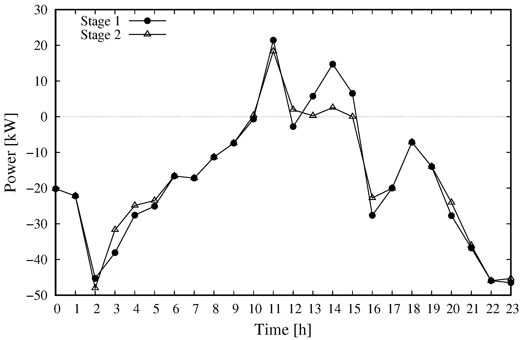
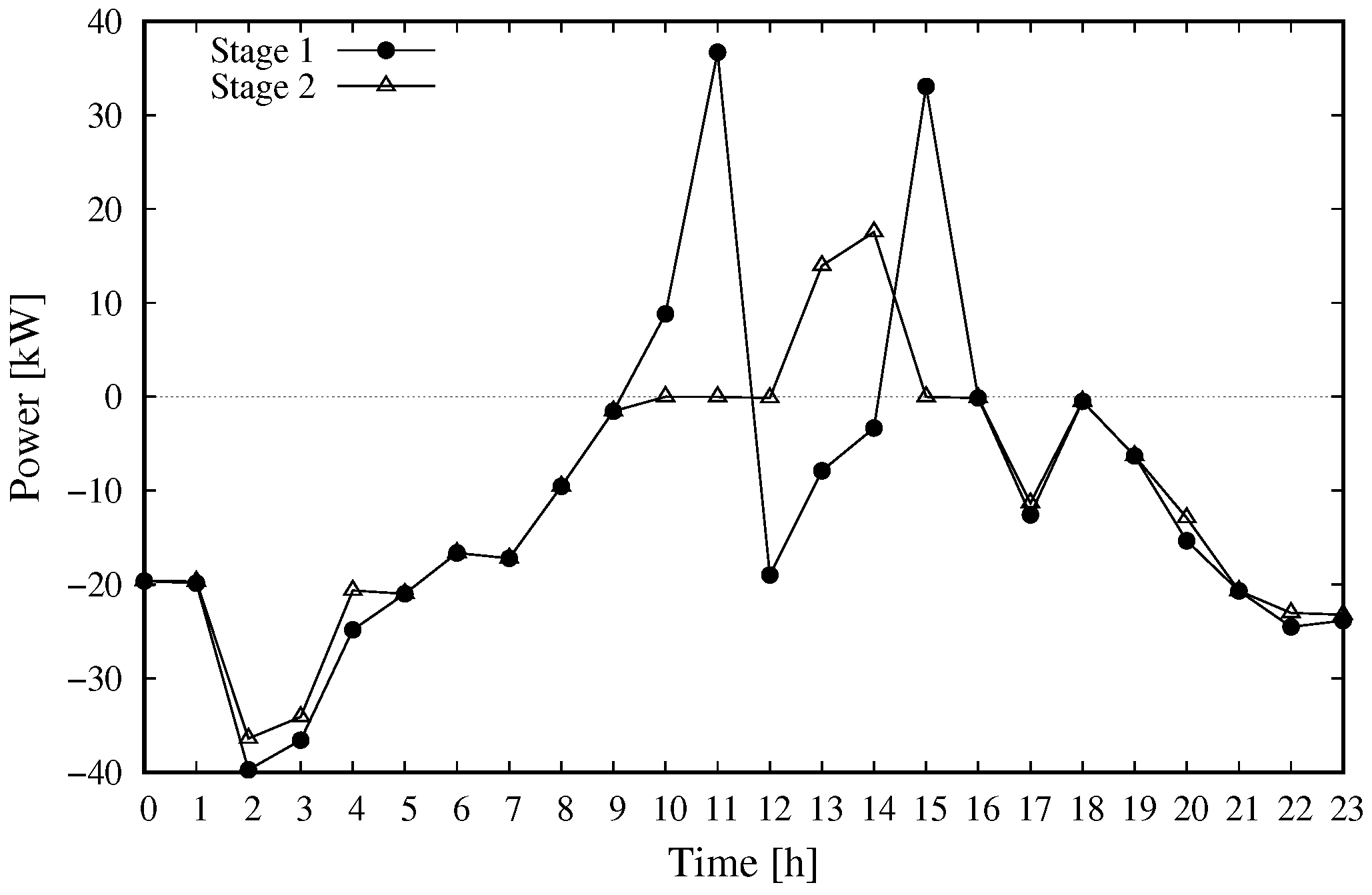
In Case A, all prosumers and consumers belong to a single category, and the values of loads and PV plants are extracted from the same probability distribution, as explained in the previous section. As a result, the energy profiles of the groups are all similar to each other. Figure 5 shows the aggregate profile of an energy community of 100 users, computed at the end of the first and second stages. The users are partitioned into groups of 10 users each. The main difference between the two profiles is noticed between 13:00 and 16:00—the energy surplus is redistributed in the second stage and therefore is not injected to the grid. Conversely, the energy surplus between 11:00 and 12:00 is not redistributed, and the profiles of the two stages are comparable. Overall, the second stage does not enable a complete energy sharing within the community during the considered day. This is due to the homogeneity of the groups: none of the groups produces/requires an amount of energy which is remarkably higher than other groups.

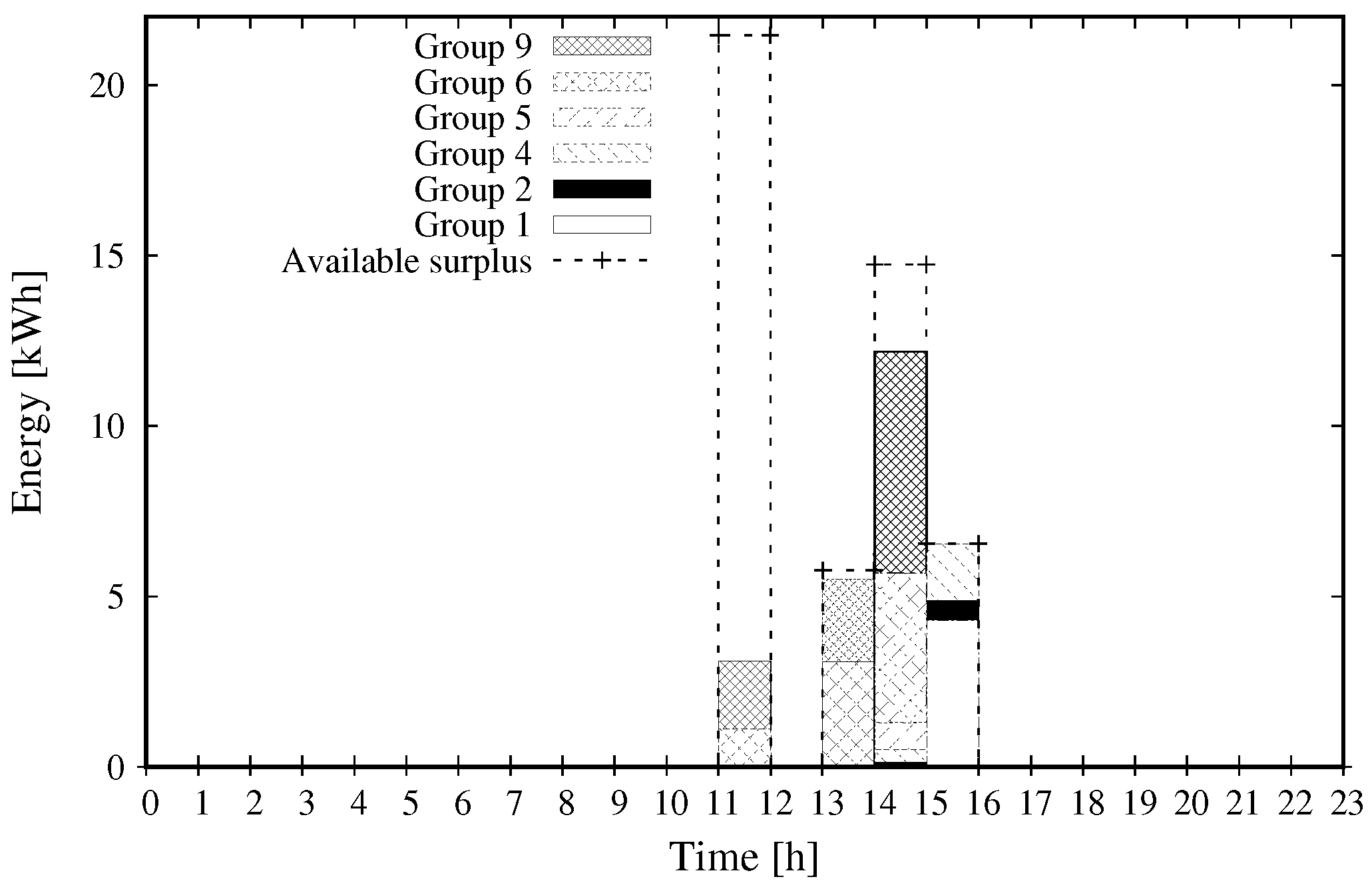
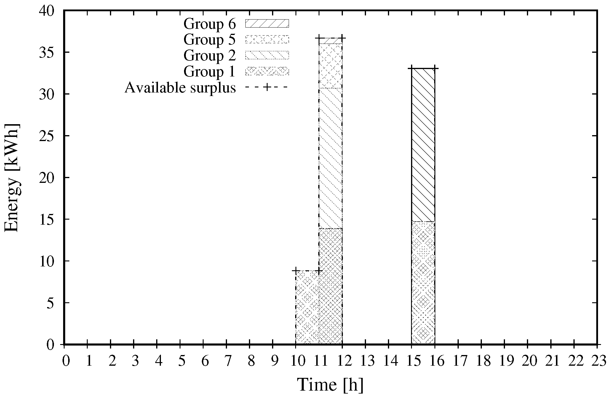
Figure 6 shows the amount of energy surplus computed after the first stage and the redistribution of this surplus to other groups. In particular, between 11:00 and 12:00, Group 6 and Group 9 acquire a fraction of the available energy surplus, while, between 13:00 and 16:00, the amount of surplus energy is almost completely redistributed, and assigned to the groups specified in the figure.

Table 4. Energy cost incurred by the single groups and the community, after the first and second stages, when considering the energy exchanged with the external grid.

Stage		First	Second
Partial cost [€] paid by	Group 1	8.903	8.218
	Group 2	5.913	5.884
	Group 3	7.512	7.512
	Group 4	4.727	4.405
	Group 5	12.729	12.700
	Group 6	7.917	6.526
	Group 7	5.895	5.895
	Group 8	12.829	12.829
	Group 9	8.958	7.254
	Group 10	9.803	9.803
Community cost [€]		85.239	81.025

reports the daily costs incurred by the different groups and the whole community after the two stages, when considering the energy exchanged with the external grid. The cost for the entire community reduces from EUR 85.24 (1° stage) to EUR 81.03 (2° stage), with a savings of about 4.94%.

Table 5. Computing time to perform the first and second stages.

Stage		First	Second
Execution time [ms]	Group 1	854	994
	Group 2	702	963
	Group 3	664	957
	Group 4	594	905
	Group 5	657	657
	Group 6	606	895
	Group 7	607	919
	Group 8	646	1040
	Group 9	711	1000
	Group 10	694	1090
Max time [ms]		854	1090

reports the time needed to execute the first and second stages in all groups. Since the groups execute, in parallel, the time to complete each of the two stages is given by the maximum computing time experienced by the groups, in this case, Group 1 for the first stage and Group 10 for the second stage. The overall computing time is the sum of these maximum times.

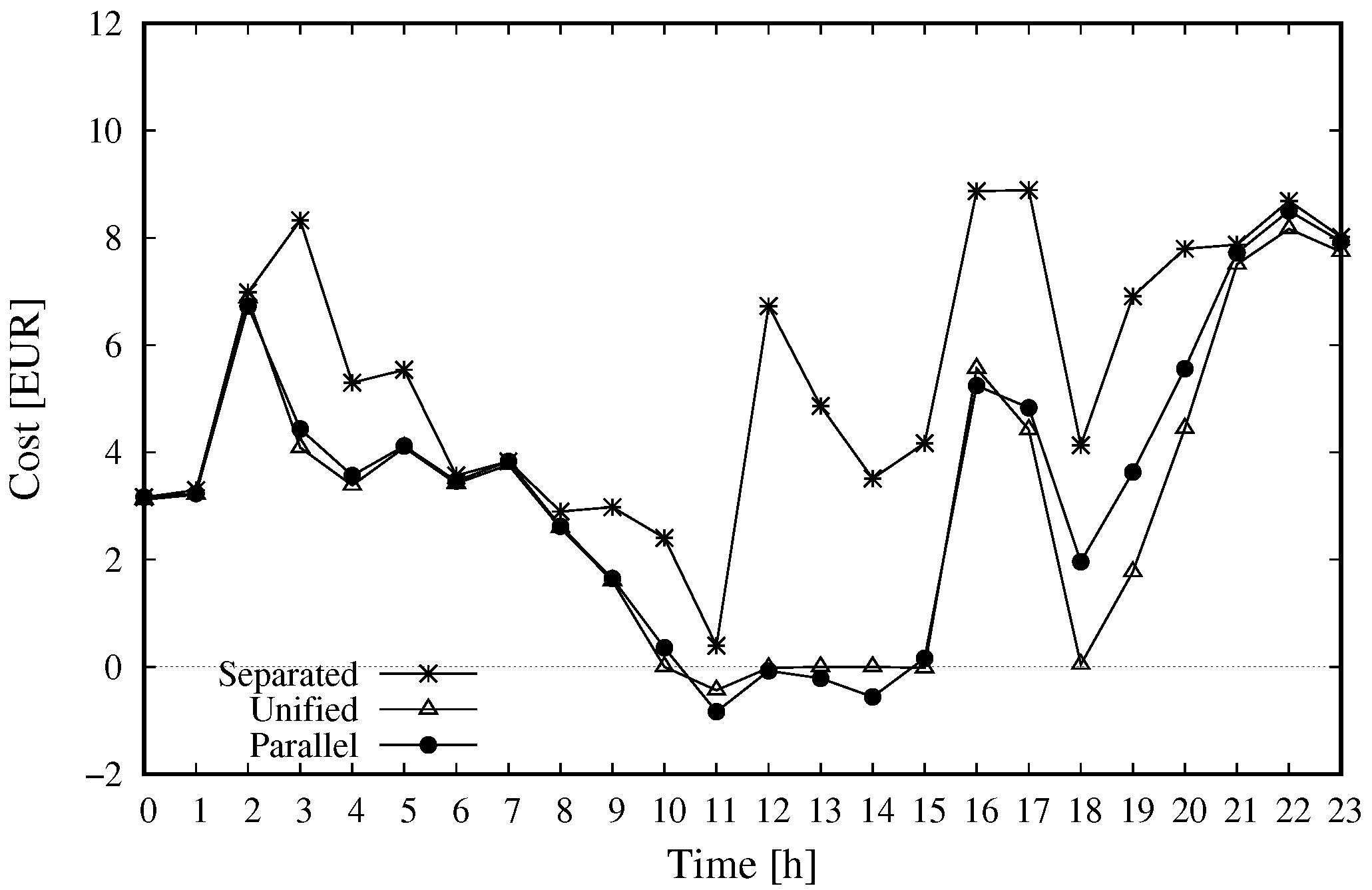
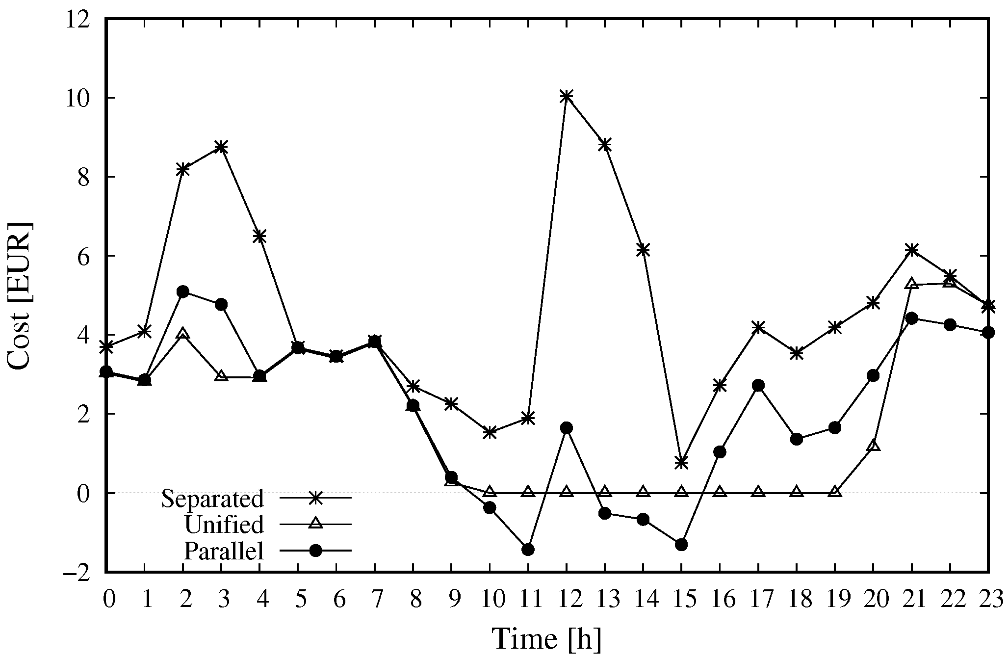
Figure 7 shows the hourly cost afforded by the community when using the three approaches considering the energy exchanged with the external grid, while

Table 6. The daily cost and execution time for a community of 100 users.

	Separated	Unified	Parallel
daily cost	EUR 129.128	EUR 75.339	EUR 81.025
execution time	123 ms	16,034 ms	1687 ms

reports the total cost for the day (in all results concerning cost, positive values are actual costs while negative values are revenues). The lowest cost is ensured by the Unified approach, which optimizes the scheduling plans of all users. The Parallel approach presents a small increase in costs concerning the Unified approach, about 7%, and a large reduction concerning the Separated approach, about 37%. Table 6 also compares the overall computing times of the three approaches. We see that the computing time of the Parallel approach, i.e., 1944 ms, is larger than the time spent by the Separated approach and much shorter than the time needed by the Unified approach.

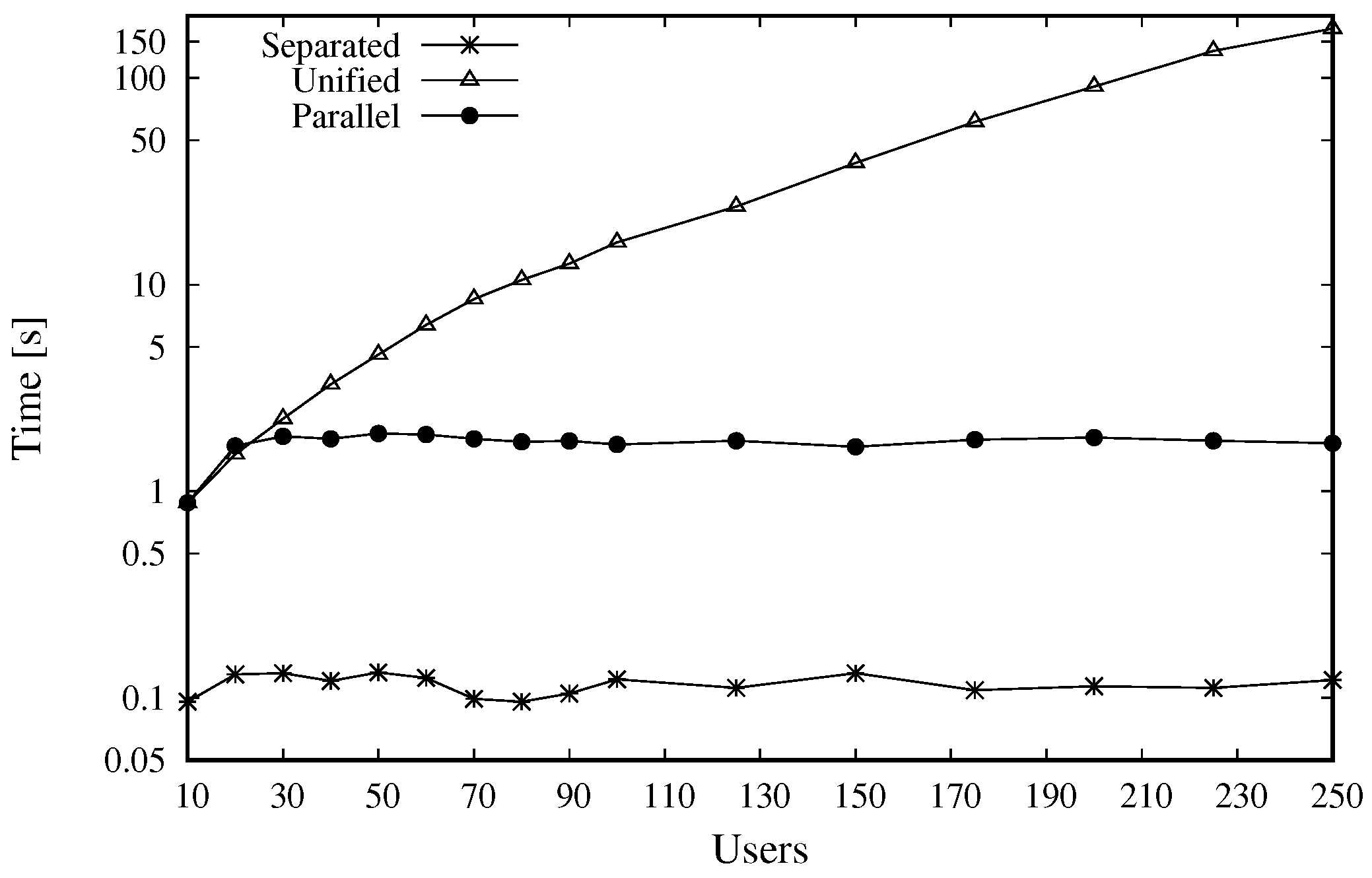
This result is confirmed by Figure 8, which compares the three approaches when varying the number of users between 10 and 250, with the group size set to 10. The figure shows that the computing time of the Unified approach increases with the number of users since the prosumer problem needs to consider all the users. With more than 100 users, the slope becomes nearly constant, which means that the increase is nearly exponential since the graph is logarithmic. In large communities, the computing time is much longer than the time needed by the Parallel approach, which is nearly constant, since all the prosumer problems involve 10 users. The times experienced by the Parallel and Unified approaches with 10 and 20 users are comparable for two different reasons: with 10 users and a single group both approaches solve a single-stage problem. With 20 users, the Unified approach executes a single-stage problem with 20 users, while the Parallel approach executes two stages and, at each stage, it solves, in parallel, two prosumer problems with 10 users. The Separated approach is the fastest one since all the users execute it in autonomy, and each user needs to solve a problem with a limited number of variables and constraints. We have seen before, however (Figure 7 and Table 6), that this approach leads to a poor solution in terms of costs.

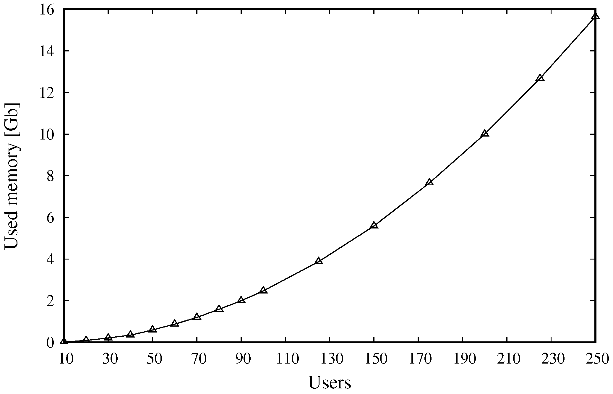
With the Parallel approach, the amount of memory depends on the size of a single group and does not increase with the size of the community as with the Unified approach. Figure 9 shows the amount of memory needed by the Unified approach, which scales quadratically since the problem matrix contains a number of rows (variables) and columns (constraints) that increase linearly with the number of users. This means that the available memory (16 GB) is filled up when increasing the size of the community, which makes the solution unfeasible for more than 250 users.

We can conclude that the Parallel approach reaches the goal for which it has been devised: it finds a solution that is very close to the optimal one (achieved with the Unified approach) in terms of costs/revenues, but with an amount of time and memory that is much lower and, which is crucial for large communities, almost constant with respect to the number of users. On the other hand, the Separated approach is not demanding in terms of computing resources but does not exploit the benefits deriving from energy communities, and leads to a very poor solution in terms of energy costs.

6.2. Heterogeneous User Groups

In Case B, the users are partitioned into two categories, as explained in Section 5. In this scenario, the second stage of the Parallel approach enables a notable reduction of the energy costs concerning the first stage. The reason is that the presence of users with different characteristics gives more possibilities to redistribute the energy surplus observed in the first stage. Figure 10 shows the aggregate daily profile of an energy community of 100 users, observed for Case B. As in Case A, at the end of the first stage, there is a surplus of energy in two-time bands, between 10:00 and 12:00 and between 15:00 and 16:00. Meanwhile, between 12:00 and 15:00, an amount of energy is absorbed from the grid because some consumers schedule their loads in those hours when the energy cost has a local minimum (see Figure 4). In the second stage, the consumers reschedule some of their loads in the surplus hours, and in this way, they exploit the energy produced locally. Indeed, a large fraction of the surplus is efficiently redistributed, and the amount of energy exchanged with the grid is greatly reduced. This is confirmed in Figure 11, which shows that practically all the available surplus is redistributed to the single groups.

Table 7. Case B. Energy cost incurred by the single groups and the community, after the first and second stage.

Stage		First	Second
Partial cost [EUR] paid by	Group 1	12.646	6.019
	Group 2	12.138	5.836
	Group 3	1.652	1.652
	Group 4	3.057	3.057
	Group 5	6.699	5.942
	Group 6	9.142	9.048
	Group 7	6.028	6.028
	Group 8	6.718	6.718
	Group 9	2.495	2.495
	Group 10	5.403	5.403
Community cost [EUR]		65.979	52.198

reports the detailed values of the daily energy costs incurred by the entire community after the execution of the two stages. It can be seen that the groups that are granted a significant amount of energy surplus are those that experience a significant cost saving at the second stage. The daily energy cost decreases from EUR 65.98 (first stage) to EUR 52.20 (second stage), with a savings equal to about 21%.

The computing times experienced with the Parallel, Separated, and Unified approaches are very similar to those obtained for Case A, and are not reported here. Indeed, though the users have different characteristics, the prosumer problems have the same size as in Case A. The main conclusion is therefore the same—the Parallel approach enables a notable reduction of the computing time with respect to the Unified approach.

Figure 12 shows the hourly cost afforded by a community of 100 users when using the three approaches. We see that the Unified approach brings the energy costs, and the energy exchanges with the external grid to zero in a long time interval between 10:00 and 20:00, while some energy exchanges with the grid are required with the Parallel approach. With the latter approach, time intervals alternate in which the energy costs are negative (corresponding to revenues) and positive (actual costs). Overall, the daily cost of the Parallel approach is slightly higher, as shown in

Table 8. Case B. The daily cost for a community of 100 users.

Separated	Unified	Parallel
112.230 €	45.504 €	52.198 €

.

When compared to Case A (see Figure 7), the difference between the Parallel and the Unified approach is higher—it is about 13% in Case B while it was 7% in Case A. This difference comes from the heterogeneity of the groups in Case B, which is handled more efficiently when all the users are taken into account by a single prosumer problem. It is confirmed that the Separated approach leads to a much larger cost, since there is no opportunity of sharing the energy among the users of the community.

As a conclusive comment for this set of experiments, we have found that the Parallel approach enables a significant saving in terms of computing time with respect to the Unified approach, at the cost of the slightly lower efficiency of energy sharing. Indeed, the Unified approach allows sharing of energy among all the users, while, with the Parallel approach, the sharing can only occur among different groups, through the redistribution of the energy surplus in the second stage. Moreover, the efficiency of the Parallel approach, in terms of energy cost, is higher when the profiles of users are homogeneous Case A. The solution provided by the Separated approach is very poor, which confirms that the presence of an energy community is highly beneficial.

6.3. Results for Large Communities

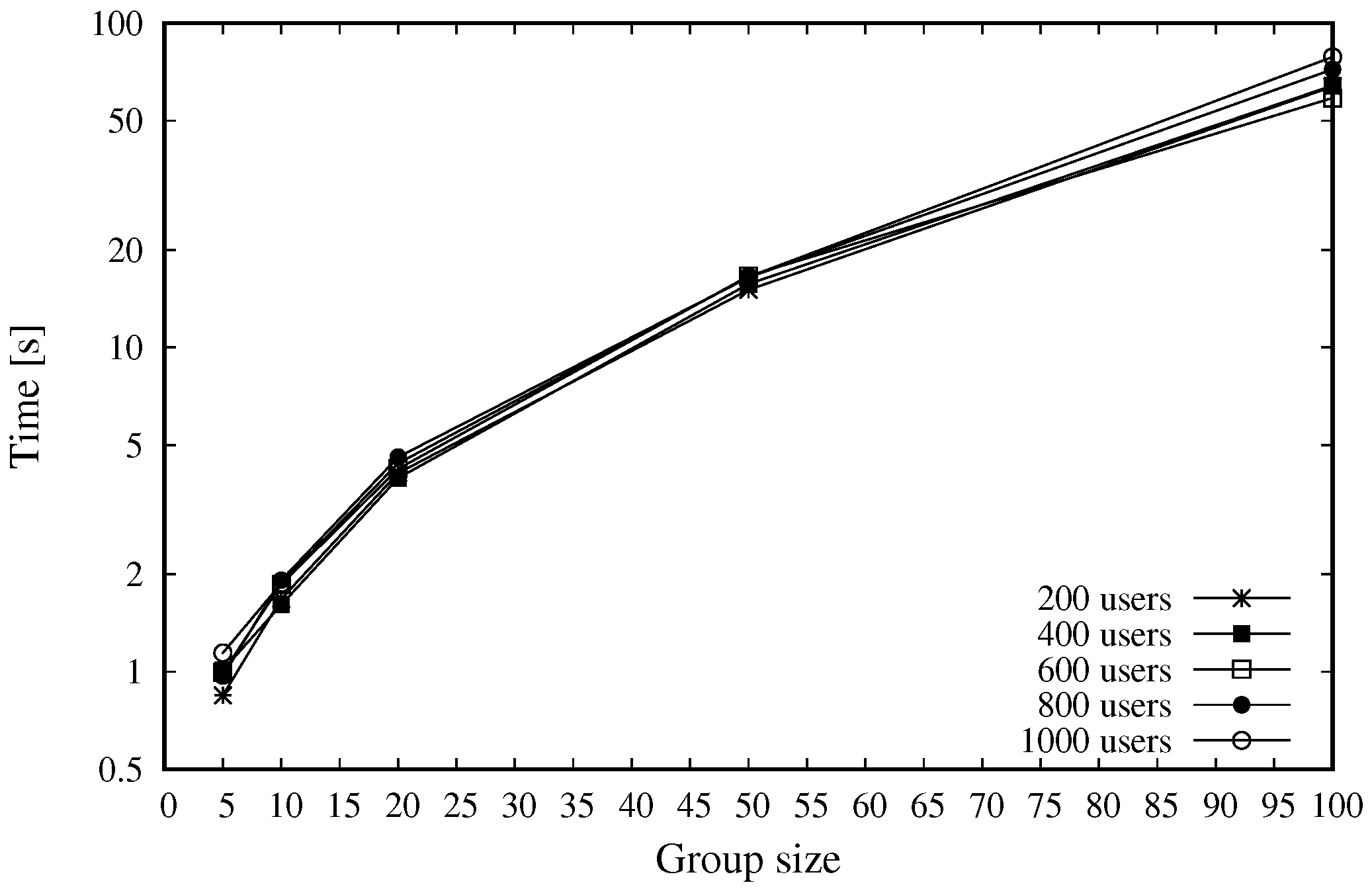
The biggest advantage of the Parallel approach is that it enables the solution of the prosumer problem for communities with very large numbers of users, which is impracticable with the Unified approach. We have seen that the hardware equipment of energy-boxes does not allow handling more than 250 users (Figure 9). To assess the scalability of the Parallel approach, we performed a number of experiments with up to 1000 users, when varying the size of the groups in which the users are partitioned. The characteristics of the users are modeled as in Case A. Figure 13 reports the computing time. We see that it increases with the group size; indeed, the prosumer problems related to the different groups are solved in parallel, and the time to solve a single problem increases with the number of users in a group. On the other hand, for a given group size, the time is nearly independent of the overall number of users, which confirms that the Parallel approach is highly scalable.

Figure 14 reports the results in terms of the overall cost. As expected, the cost is proportional to the total number of users. Conversely, the cost slightly decreases when increasing the group size, because the prosumer problem becomes more efficient when it can consider the requirements of a larger number of users in the same group.

7. Conclusions

In this paper, we have presented a Parallel computing strategy for the management of energy in large communities. The approach consists of organizing the users into groups and solving the prosumer problems for the different groups in parallel. An edge computing architecture is exploited, where the single users, the super-users that coordinate the groups, and the central energy aggregator, are associated, respectively, with smart meters, edge nodes equipped with energy boxes and a control center.

A set of experiments were performed for two scenarios: in the first, the prosumers are homogeneous; in the second, they belong to two different categories with different requirements and equipment. The results show three important outcomes: (i) the Parallel approach enables a significant redistribution of energy among the groups, thus exploiting the advantages offered by the energy community; (ii) the requirements in terms of computing time and memory are much lower than those experienced with the Unified approach, which solves a single big optimization problem, and the solution in terms of energy cost is close to the optimum; (iii) the Parallel approach is highly scalable and can be used for very large communities, since the computing requirements are given by the size of the single groups, not by the size of the entire community.

Future Work

The main limitation of the approach is the management effort that is needed to organize the groups and equip each super-user with adequate plug-and-play devices, user interfaces, and software tools. However, given the increasing worldwide success of energy communities, and the urgent need for reducing the consumption of energy, very likely, this possible limitation will be overcome soon. A promising avenue for future work concerns the real-time management of energy management. The objective is to handle the real-time deviations of load and production profiles with respect to those predicted or declared by the users, in order to prevent any significant reduction in the savings and/or revenues expected by the prosumers and by the system. This opportunity can be fostered by the use, on edge nodes, of hardware acceleration platforms specialized for the training and execution of artificial intelligence algorithms, for example, based on the reinforcement learning paradigm [45]. Furthermore, the parallel computing approach presented in this paper can enable and speed up the deployment of an energy market infrastructure [35], where multiple aggregators can buy, sell energy, and offer ancillary services that support the continuous flow of electricity.