Article

Characterizing Various Produced Waters from Shale Energy Extraction within the Context of Reuse

by
Tiffany Liden
1,
Zacariah L. Hildenbrand
2,3,*,
Ramon Sanchez-Rosario
3 and
Kevin A. Schug
1,2,*
1
Department of Chemistry and Biochemistry, The University of Texas at Arlington, 700 Planetarium Place, Arlington, TX 76019, USA
2
Collaborative Laboratories for Environmental Analysis and Remediation, The University of Texas at Arlington, Arlington, TX 76019, USA
3
Department of Chemistry and Biochemistry, The University of Texas at El Paso, 500 W. University Ave, El Paso, TX 79968, USA
*
Authors to whom correspondence should be addressed.
Energies 2022, 15(13), 4521; https://doi.org/10.3390/en15134521
Submission received: 3 May 2022 / Revised: 6 June 2022 / Accepted: 15 June 2022 / Published: 21 June 2022

Abstract

:
Environmental concerns with unconventional oil and gas development are frequently centered on elevated water usage and the induction of seismic events during waste disposal. Reuse of produced water for subsequent production well stimulation can effectively address these concerns, but the variability among such samples must be well understood. Twenty-four samples of wastewater from unconventional oil and gas development were collected from south and west Texas to assess their variability and feasibility for direct reuse. Bulk metrics were collected, including total organic carbon, total nitrogen, as well as total dissolved and suspended solids. The profiles of pertinent inorganic constituents were also evaluated. Variations were not only seen between regions but also among samples collected from the same region. For example, the average total organic carbon for Eagle Ford samples collected was 700 ± 500 mg/L, while samples collected from the Permian Basin featured an average total organic carbon concentration of 600 ± 900 mg/L. The Permian Basin total organic carbon ranged from 38 to 2600 mg/L. The total dissolved solids levels had the same variability between regions, with an average value for Eagle Ford of 20,000 ± 10,000 mg/L and a Permian Basin value of 150,000 ± 40,000 mg/L. However, samples were more reproducible within a given region. Collectively, the data indicate that the direct reuse of raw produced water for subsequent production well development without treatment is not feasible based on the reported reuse thresholds. Unconventional development wastewater samples from the Permian Basin were also compared to produced water values from conventional oil and gas wells in the same region, as reported by the United States Geological Survey. Samples collected in the Permian Basin consistently demonstrated lower ionic strength compared to conventional produced water data.

1. Introduction

Unconventional oil and gas development (UD) provides the fossil fuel necessary to meet the majority of the ever-growing energy needs in the United States [1,2,3]. This highly articulated process requires large amounts of water to extract oil and natural gas from formations previously considered to be uneconomical [4]. Upon stimulation with hydraulic fracturing (HF), the primary by-product of UD is a waste stream composed of flowback (FB) and produced water (PW). The FB is predominantly a stimulation fluid returning to the surface, which contains some dissolved minerals, as well as chemical additives used during the HF process. FB is a minor component of the total wastewater produced by a well. Its return to the surface lasts for 1–2 weeks, once production begins. In contrast, the production of PW, the major component of the waste stream, continues over the lifetime of the well. It is brought to the surface comingled with the commodity and contains increased levels of dissolved minerals that are reflective of the mineral composition of the petroliferous strata of interest. In addition to the elevated levels of salts (sodium and chloride) and scaling elements (calcium, magnesium, strontium, and barium), PW also contains a plethora of aerobic and anaerobic bacteria [5] and aromatic and alkyl hydrocarbons of varying sizes [6].
In 2011, 4.9 billion gallons of water was used to stimulate unconventional wells in Texas, which accounted for less than 1% of the state’s water usage [7,8]. More recent data from 2017 suggest that over 55 billion gallons of water was used for HF in the Permian Basin alone [9]. Overall, the volume of water used is low compared to other anthropogenic activities (i.e., agriculture and farming), but UD frequently occurs in arid and semiarid regions [10]. Localized high-water usage can negatively impact a particular region through the development of water depletion cones. Actual water usage data can be challenging to obtain, since companies are not required to report their water usage in some regions. However, during HF, it is estimated that 5 million gallons of water is used on average for a horizontal well completion [11].
The largest expansion in water usage for HF has taken place in the Permian Basin (PB). Located in Texas and New Mexico, the PB is currently considered to be the most prolific energy basin in the world [4,12]. From 2005 to 2015, horizontal wells represented only one-third of the unconventional wells in the region, but they accounted for approximately two-thirds of the HF water used [13]. Backstrom et al. discovered that PB water usage exceeded the national average, with a median of 12 million gallons per well for stimulation [14]. Interestingly, from 2013 to 2016, the water use per well went up by approximately 434% in the PB of west Texas [15]. The increase was attributed to expanded drilling activity and completions, where the average horizontal length had increased from 5700 to 6800 lateral ft, with lateral stretches reaching up to and even over 10,000 ft [4].
Another concern associated with UD, particularly with respect to the production and disposal of PW, is the link to increased seismicity. Currently, 98% of PW is disposed of through the use of enhanced oil recovery wells and salt water disposal (SWD) wells [4,16,17]. Enhanced oil recovery is typically used for conventional development, whereas SWD is the preferred disposal option for UD because of economics and convenience [18]. However, the volume of PW injected into SWD wells has been shown to have a direct correlation to the number and magnitude of seismic events [19,20,21,22,23,24]. A recent example can be seen in Oklahoma, where the number of earthquakes increased after 2009 from an average of 1.2 events/year to 25 annually [25]. It is expected that this disposal option will continue to be subject to growing constraints and scrutiny due to increased seismic events, which could ultimately lead to significant property damage or harm to humans [26].
To mitigate the concerns associated with high water usage and induced seismic events, there is a growing need to reuse or recycle PW. The ability to reuse PW is primarily dependent on the concentration of inorganic constituents [5,6,27,28]. The thresholds of constituents of concern typically found in PW are listed in Table 1. In this study, 24 PW samples were collected from the south and west Texas regions to compare inorganic matrices and total organic content, to ultimately characterize the different PW samples and determine the feasibility of their direct reuse for production well stimulation. To date, the collection of FB and/or PW samples for compositional analyses is extremely challenging due to varying concerns from oil and gas operators regarding the maintenance of trade secret formulations of their HF fluid additives and the productivity rates of their UD wells. Additionally, there have been limited data regarding the composition of PW from UD, in part due to the challenges in accessing it. Therefore, PB samples were also compared with USGS PW data from the PB region from conventional oil and gas development to determine if past samples could potentially be a predictor of the relative composition of the PW from UD.

2. Methods and Materials
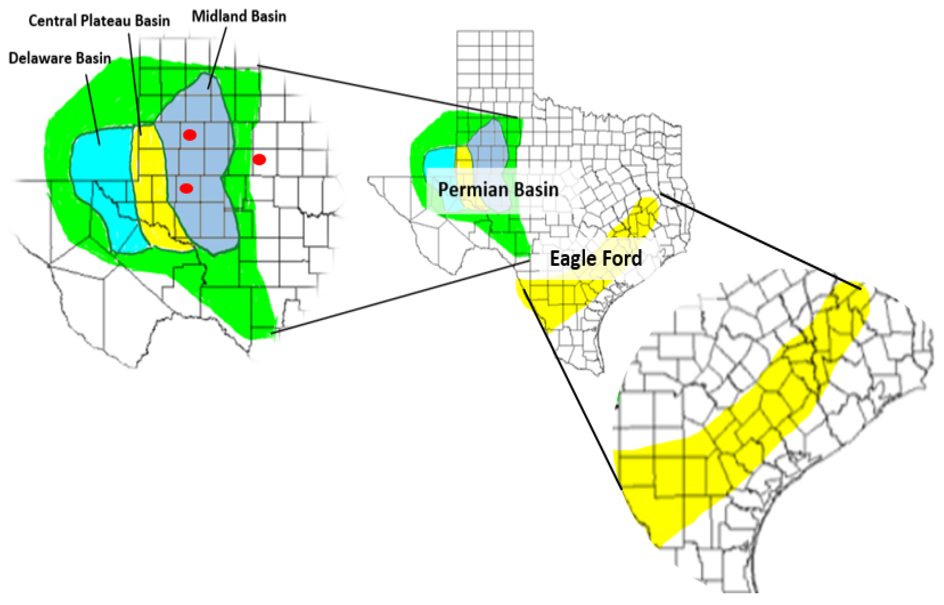
2.1. Samples

Nine of the samples used were collected from the PB in west Texas (Figure 1). One sample (PB FB), classified as FB because of its age and chemical composition [6], was collected from an unconventional oil exploration on-site waste pit, approximately one week after well completion. Eight samples, collectively referred to as PB SWD, were collected from a saltwater disposal site (SWD) located in the PB. Seven were from a site in Midland County, and one was from a site in Dawson County. The PW from Midland County was a composite mixture, delivered to the specific SWD site by six pipelines, as well as trucks purported to be from production sites up to 50 miles away. The PW collected in Dawson County was also from a community SWD well, similar to the Midland site, except that all of the PW was delivered to the site by truck. It is important to note that the PB samples could potentially be a mixture from multiple sites producing conventional and unconventional oil and gas wells. However, the SWD operator clearly indicated that the wastewater was from UD operations. The remaining sample set, denoted as EF Treatment, included 13 samples of PW from a treatment facility located in Eagle Ford Shale in Bebe, TX [5]. Two samples, denoted as EF wells, were from production wells located in Brazos County and were collected before separating the PW from the oil.

2.2. Compositional Analyses

Total suspended and dissolved solids were quantified using gravimetric analysis. PW samples were filtered using Ahlstrom 1 µm Glass Microfiber Paper (Leominster, MA, USA) and dried overnight at 90 °C. Metal analysis was completed using a Shimadzu ICPE-9000 (Columbia, MD, USA), based on Environmental Protection Agency (EPA, Washington, DC, USA) method 200.7. Standard solutions for the metals were from High-Purity Standards (North Charleston, SC, USA). Ion chromatography (IC) and titration were used to quantify pertinent anions, as per EPA methods 300 and 310.1. Total organic carbon (TOC) concentrations were determined using a Shimadzu TOC-L (Shimadzu Scientific Instruments, Inc., Columbia, MD, USA), as described previously [6,30,31].

3. Results and Discussion

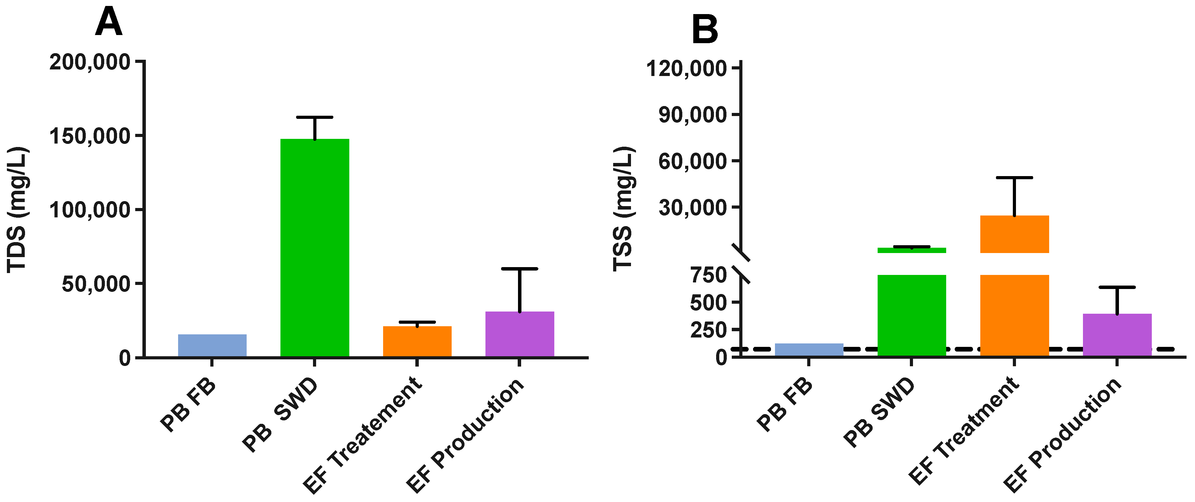
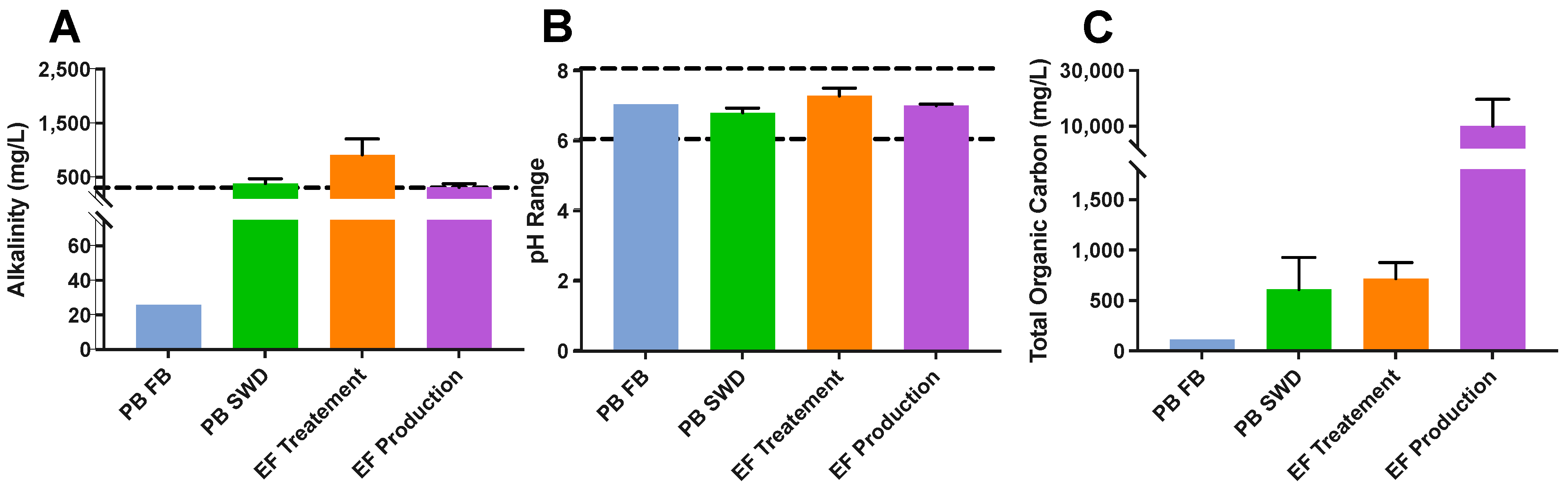
3.1. Bulk Measurements and Basic Parameters
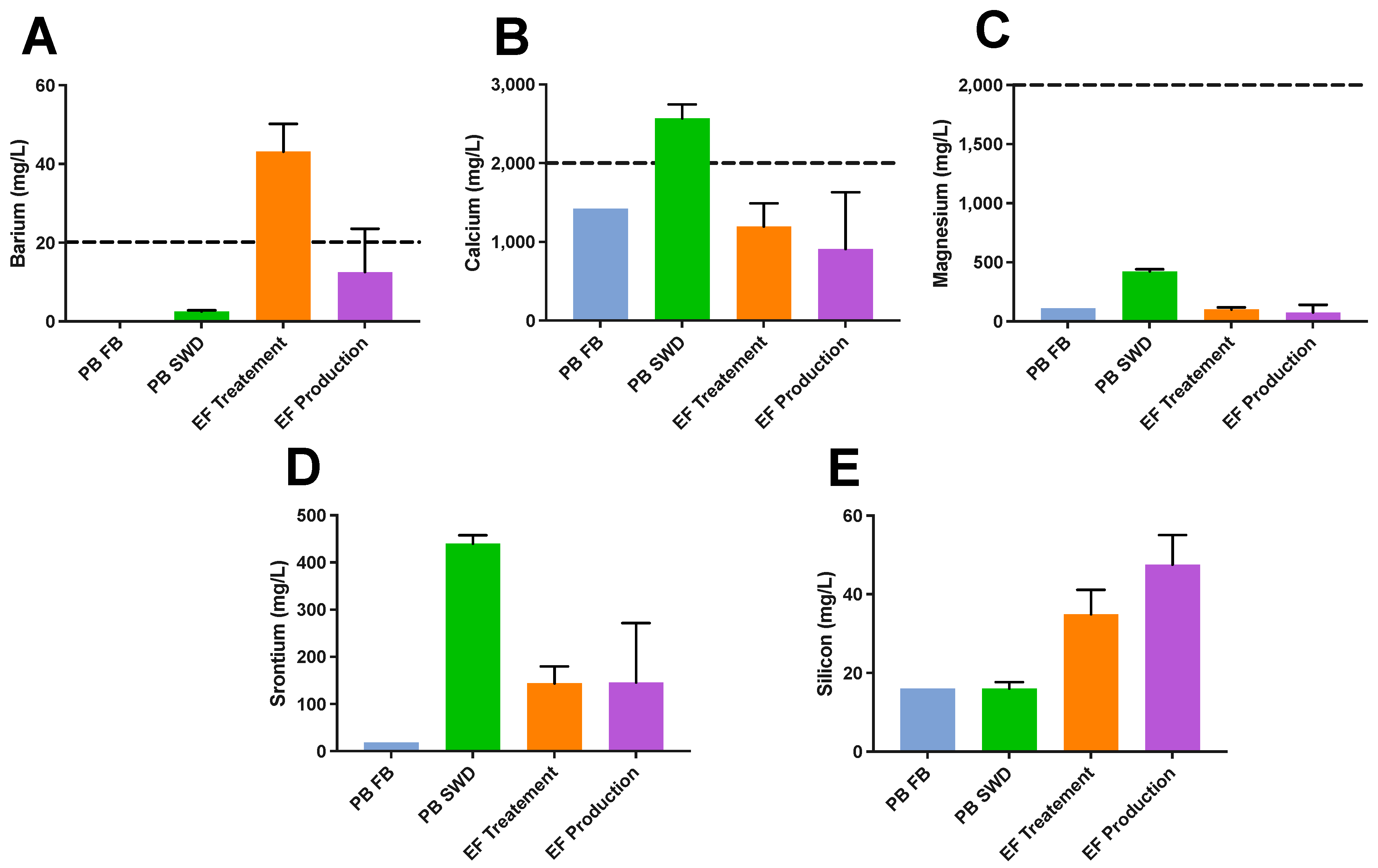
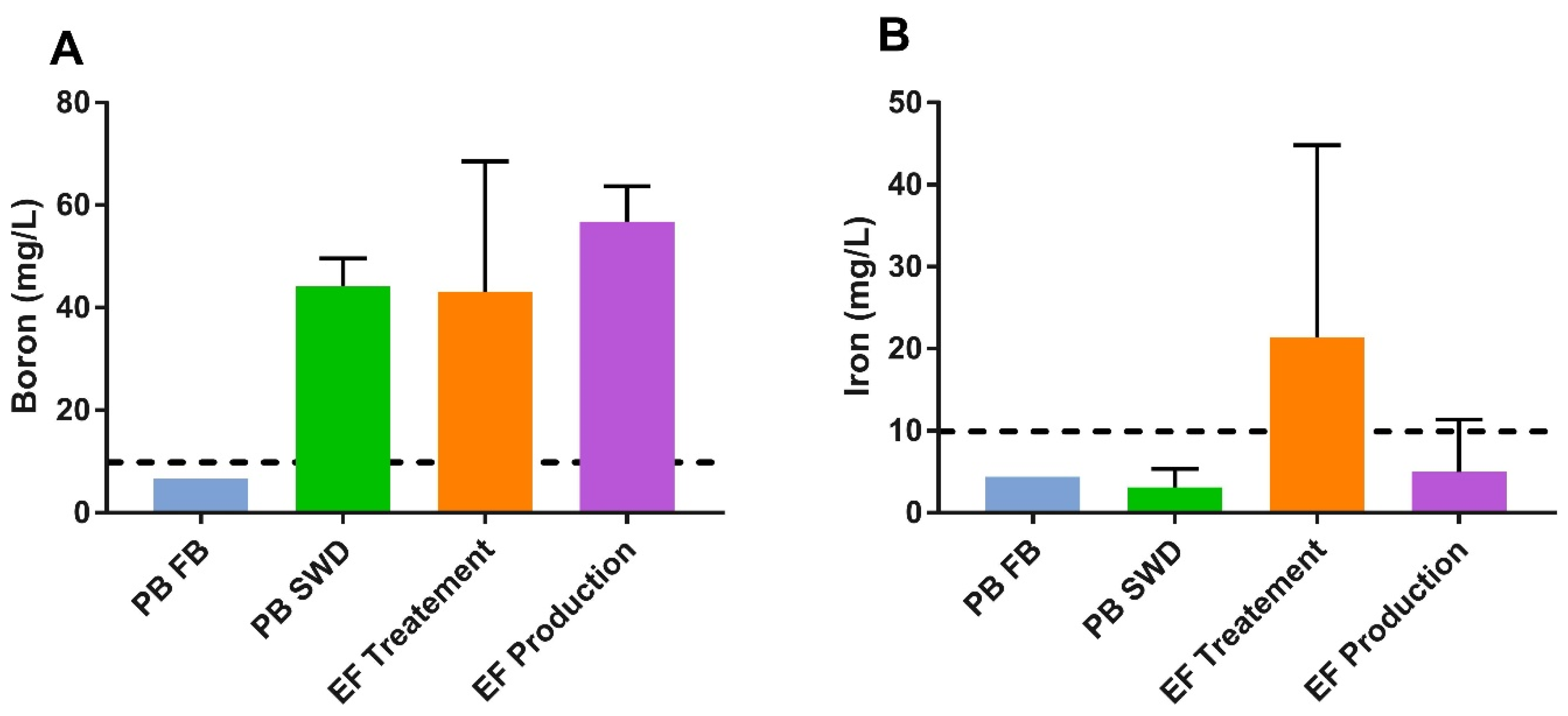
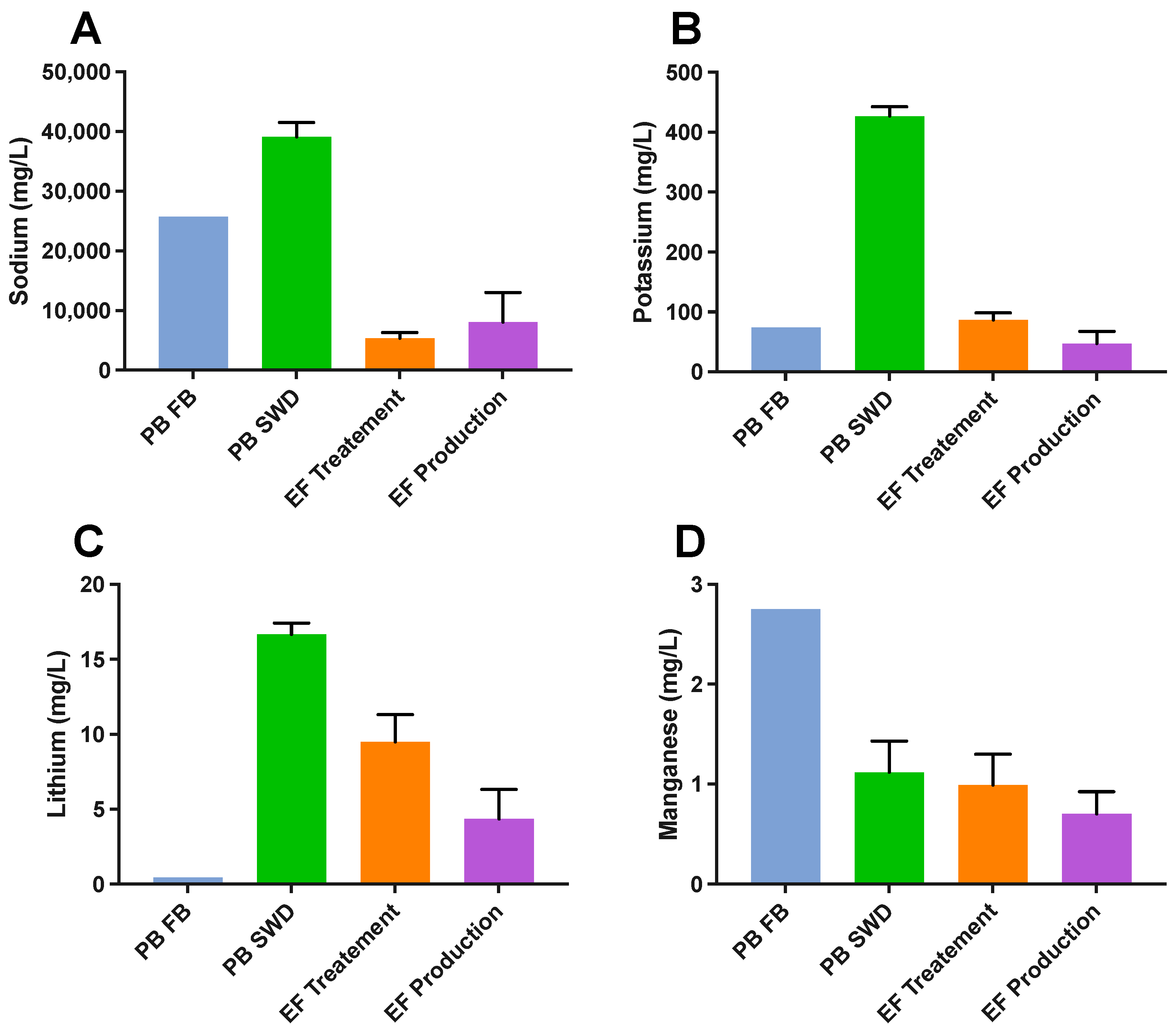
The measurement of total dissolved solids (TDS) corresponds to the number of dissolved particles in solution. Values can range from freshwater levels (<1000 mg/L) through saline (15,000–30,000 mg/L) to brine (>300,000 mg/L) [32]; however, values are relatively inconsequential with respect to reuse for production well stimulation. Notably, samples collected from the PB SWD ranged from 10 to 12% salinity, with an average TDS value of 150,000 ± 40,000 mg/L. The samples collected from the EF region ranged from 2 to 5% salinity, which is roughly equivalent to seawater (SI Table S1). Similarly, total suspended solids (TSS) is a simple bulk measurement that can provide significant insight into the nature of the particulates in a solution. Typically, components such as oil droplets, flocculated hydrocarbons, formation sands, and proppants that are greater than 1 μm in size, contribute to the measurement of TSS. Ideally, TSS should be less than 500 mg/L for reuse (Table 1). Figure 2B indicates that TSS levels exceeded the reuse limit for both the PB SWD set and the EF treatment samples. For the EF treatment samples, the average was skewed due to one sample reaching 220,000 mg/L (SI Table S1). The remaining 12 samples were near or below the accepted reuse levels, ranging from 50 mg/L to 780 mg/L. On the other hand, the TSS levels for the PB SWD samples were typically higher than the EF treatment samples; values ranged from 300 to 6100 mg/L.
A viable alkalinity threshold (carbonate + bicarbonate) to determine whether or not PW is suitable for reuse is considered to be 300 mg/L (Table 1). Alkalinity not only influences the pH due to its buffering capacity, but it also contributes to scaling, which is a primary concern with respect to PW reuse [33]. Scale formation is problematic because it can have devastating financial implications throughout the lifecycle of production [28]. Figure 3A shows alkalinity was only 26 mg/L for the PB FB but ranged from 74 to 840 mg/L for the PB SWD samples. The samples from the EF treatment facility had a similar range, from 170 to 910 mg/L for 11 of the 13 samples, with the remaining 2 reaching as high as 2200 and 4000 mg/L, respectively.
The pH was within an acceptable range for reuse (6–8) for all of the collected samples (Figure 3B). The defined maximum reuse levels for TOC have not been published, as far as the authors are aware. However, anecdotal feedback from the PB SWD operator indicated that TOC values above 20 mg/L were unfavorable when considering potential reuse for production well stimulation. All average values of each of the PW sample sets exceeded this threshold. The average TOC value was highest for samples from the EF production wells (Figure 3C). However, given the significant variability, with one sample having a TOC value of 20,000 mg/L and the other 380 mg/L (SI Table S1), the average value does not provide the most representative insight. Samples collected from the EF treatment center ranged from 240 to 1500 mg/L (SI Table S1). The eight PB SWD samples ranged from 38 to 2600 mg/L (SI Table S1).

3.2. Metals

The salinity of PW is a result of dissolved ions, primarily sodium and chloride [34]. To a lesser extent, other cations and anions influence the salinity, such as calcium, magnesium, and sulfate, as well as those that influence the alkalinity of the solution. Ions that contribute to scaling are the most pertinent metals to determine with respect to PW reuse for production well stimulation, followed by those that affect crosslinker efficiency, and lastly, ions, which are of lesser consequence and only influence the TDS levels.
Scaling concerns are dominated by multivalent cations [28], where barium, calcium, magnesium, and strontium are at the forefront of this issue. Barium from the formation can result in the precipitation of barium sulfate scale [35].As the pressure and temperature decrease when the PW is brought to the surface, the solubility of barium sulfate decreases, leading to scale formation [36]. As such, an acceptable level of barium for reuse is 20 mg/L (Table 1, Figure 4A). Sample sets from the EF region exceeded this threshold, with averages of 35 mg/L and 48 mg/L for the EF treatment and EF production well samples, respectively. In contrast, the PB SWD sample set had a mean value of 16 mg/L. Barium is not a stimulation additive, as far as the authors are aware. Therefore, it is not surprising that it was not detected in the PB FB samples, which were expected to be predominately composed of stimulation fluid.
Calcium and magnesium both have suggested limits of 2000 mg/L (Table 1). All but one of the samples collected from the PB SWD exceeded the recommended reuse level for calcium. Samples ranged from 1600 mg/L to 3000 mg/L, with an average value of 2600 mg/L; however, all of the other samples fell below the threshold. This is shown in Figure 4B. All of the average values for each sample set fell below the prerequisite limit for magnesium (Figure 4C). Further, strontium behaves similarly to barium in the presence of sulfate and under similar conditions; however, strontium sulfate is slightly more soluble than barium sulfate [36]. Samples from the EF treatment facility and EF production wells exhibited similar strontium concentrations, as expected, with averages of 140 mg/L and 150 mg/L, respectively (Figure 4D). Conversely, the samples from the PB SWD site, with an average value of 440 mg/L, contained three times the concentration of strontium compared to the EF samples.
Silica, monitored as silicon, can also lead to scaling concerns when present. While there is not a limit set for silicon, highly saline environments, such as PW, can enhance scale formation by silica [37]. In regions such as west Texas, where silica can cause up to 80% of scale formation [36], silica is a major concern. Interestingly, silicon levels for the EF sample sets had higher average values than the PB SWD samples (16 mg/L), with average values of 35 and 48 mg/L observed in the EF treatment and production samples, respectively (Figure 4E).
Crosslinkers or viscosifiers are used to increase the molecular weight by crosslinking a polymer backbone, thereby extending the distance to which the proppant can be placed within the fractured formation [38]. Typically, these compounds are formed from metals, such as boron, titanium, or zirconium, which have been conjoined by ligands [38,39]. Zirconium and titanium were not detected in any of the samples. Nonetheless, each of the three PW averages exceeded the 10 mg/L limit for boron (Figure 5A). Additionally, iron levels exceeding 10 mg/L can cause over-crosslinking and adversely affect the temperature stability of fracturing fluid (Table 1). The average iron concentration for the EF samples from the treatment facility, represented in Figure 5B, surpassed the limit, with an average value of 22 mg/L. However, these samples exhibited significant variability, with values ranging from 0.5 to 68 mg/L, with 6 of the 13 samples surpassing the reuse limits (SI Table S2). Samples from the PB SWD had an average value of 3.0 mg/L; however, the collection of these samples was performed after the addition of an undisclosed iron reducer.
Sodium, potassium, lithium, and manganese were also detected in all samples procured for this study. These ions affect the TDS level but have limited influence on the solution chemistry. The average concentrations of sodium (39,000 mg/L), potassium (430 mg/L), and lithium (17 mg/L) were highest for the PB SWD, which was expected due to the elevated TDS levels detected (Figure 6A–C). The PB FB had elevated levels of sodium and potassium, with values of 26,000 mg/L and 74 mg/L, respectively. As the composition of FB waste is reflective of the original stimulation fluid prepared, it is suspected that sodium and potassium chloride were used as clay stabilization additives, a common practice that began the 1960s [28,38,40,41,42,43]. Samples collected at the EF treatment facility had the most substantial standard deviation of 6.6 mg/L for lithium, with a mean of 9.5 mg/L. Relatively low levels of manganese were detected in all of the sample sets, with the highest concentrations being found in the PB FB group, with a concentration near 3.0 mg/L (Figure 6D). Manganese, like iron, can potentially be an issue when PW is brought to the surface, leading to the formation of manganese oxides, which can precipitate out of a solution, forming scale. An added benefit of oxidized manganese, in the form of permanganate, is that it can react with hydrogen sulfide (H2S) [44], thereby eliminating this harmful toxin. Hydrogen sulfide is a biodegradation product formed by sulfur-reducing bacteria (SRB). It is the primary cause of costly product quality degradation, referred to as souring, as well as biocorrosion of metal infrastructure that can potentially lead to casing failure and environmental contamination.

3.3. Anions

The anions bromide, chloride, fluoride, sulfate, and nitrate were also monitored; they are characterized by the average values indicated in Figure 7. Chlorine and chlorine dioxide, commonly used disinfectants, are known to produce toxic disinfection by-products (DBPs) [45,46,47]. However, when bromide is present in solution at concentrations as low as 0.1 mg/L, it has been shown to oxidize quickly and react with organic materials, which can lead to the formation of brominated and chlorinated DBPs. Elevated levels of bromide preferentially generate brominated DBPs [48]. While bromide was not detected in the PB FB, its concentration in the remaining samples exceeded the minimum levels for the formation of DBP. Average bromide values of 190 mg/L, 70 mg/L, and 72 mg/L were measured for PB SWD, EF treatment, and EF production sample sets, respectively (Figure 7A). Elevated levels of bromide are potentially problematic, since toxicological studies suggest that brominated DBPs are more carcinogenic compared to their chlorinated counterparts.
The ideal range for chloride is 30,000–50,000 mg/L for slickwater fracturing fluids (Table 1), which both PB sample sets surpassed. However, the PB FB only slightly exceeded this range by 1000 mg/L (51,000 mg/L) (SI Table S3). This finding, along with the increased levels of sodium and potassium, alludes to the possibility that sodium and potassium chloride are commonly used clay stabilizers [28,38,40,41,42,43], which were added to the fracturing fluid.
Fluoride concentrations, which are an essential metric regarding the formation of exotic scales, such as CaF2, were the highest for samples from the EF treatment facility and ranged from <0.034 to 28.9 mg/L. All other sample sets exhibited average values below 12 mg/L (Figure 7C). Nitrate levels were the highest in the PB SWD samples, with an average value of 46 mg/L. As for the solution chemistry, nitrate is not problematic for reuse; however, it is a nutrient for bacteria, the widespread proliferation of which can result in the formation of problematic biofilms, among other problems. All of the average values were below the reuse limit of 500 mg/L for sulfate (Table 1). A value of 220 mg/L was measured for the PB FB sample, followed by the PB SWD, EF production, and EF treatment sample sets, with values recorded at 180 mg/L, 93 mg/L, and 36 mg/L, respectively.
Elevated levels of sulfate can inhibit the effectiveness of crosslinkers, which maintain viscosity in fracturing fluids [39]. Additionally, elevated sulfate levels can induce reactions with barium, strontium, and iron in the formation water of a production well, which can result in the precipitation of BaSO4 and SrSO4 scales [35]. Lastly, sulfate can provide a substrate for SRBs that produce H2S, and this can ultimately lead to the deterioration of hydrocarbon products and production infrastructure [49].

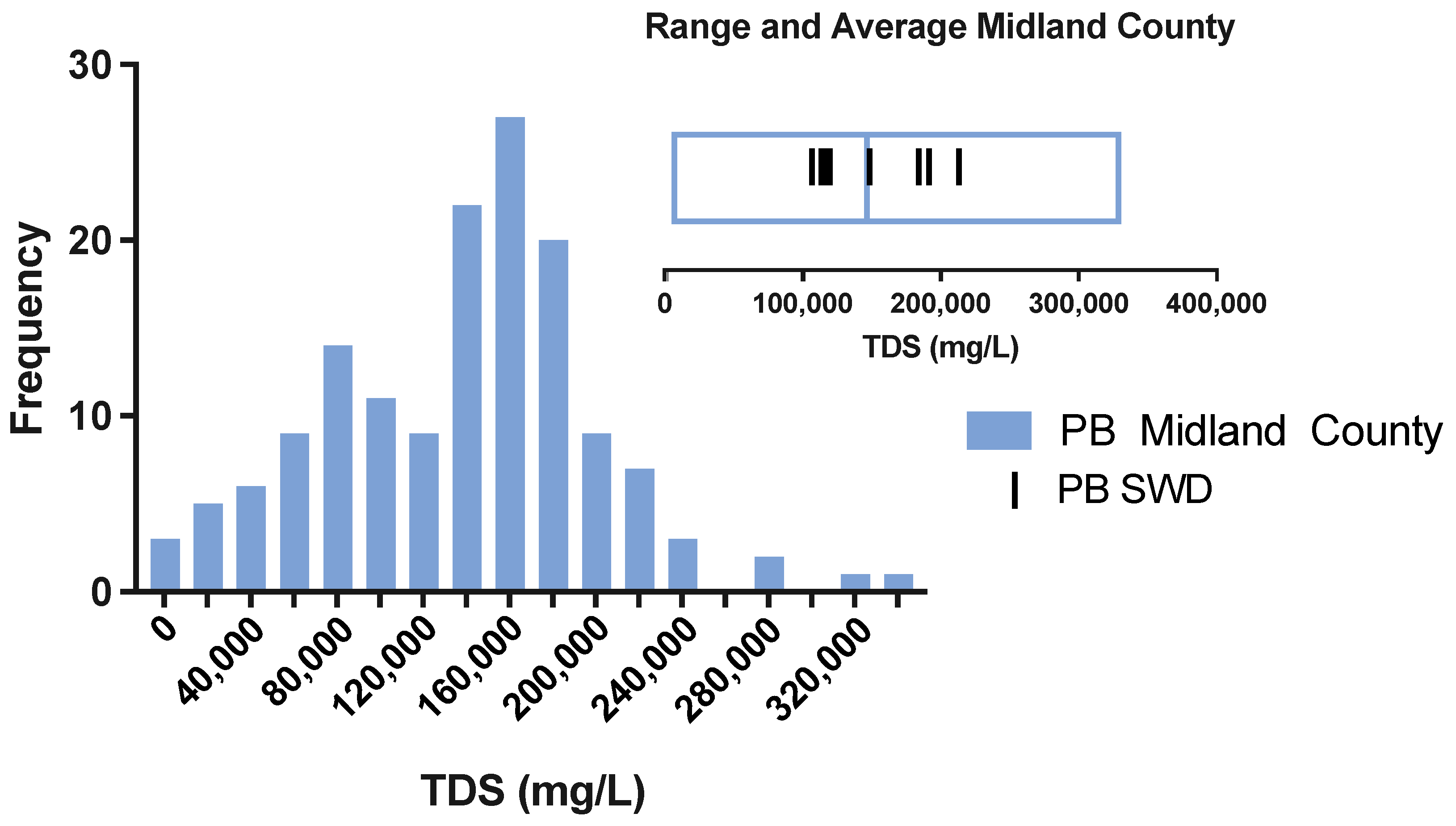
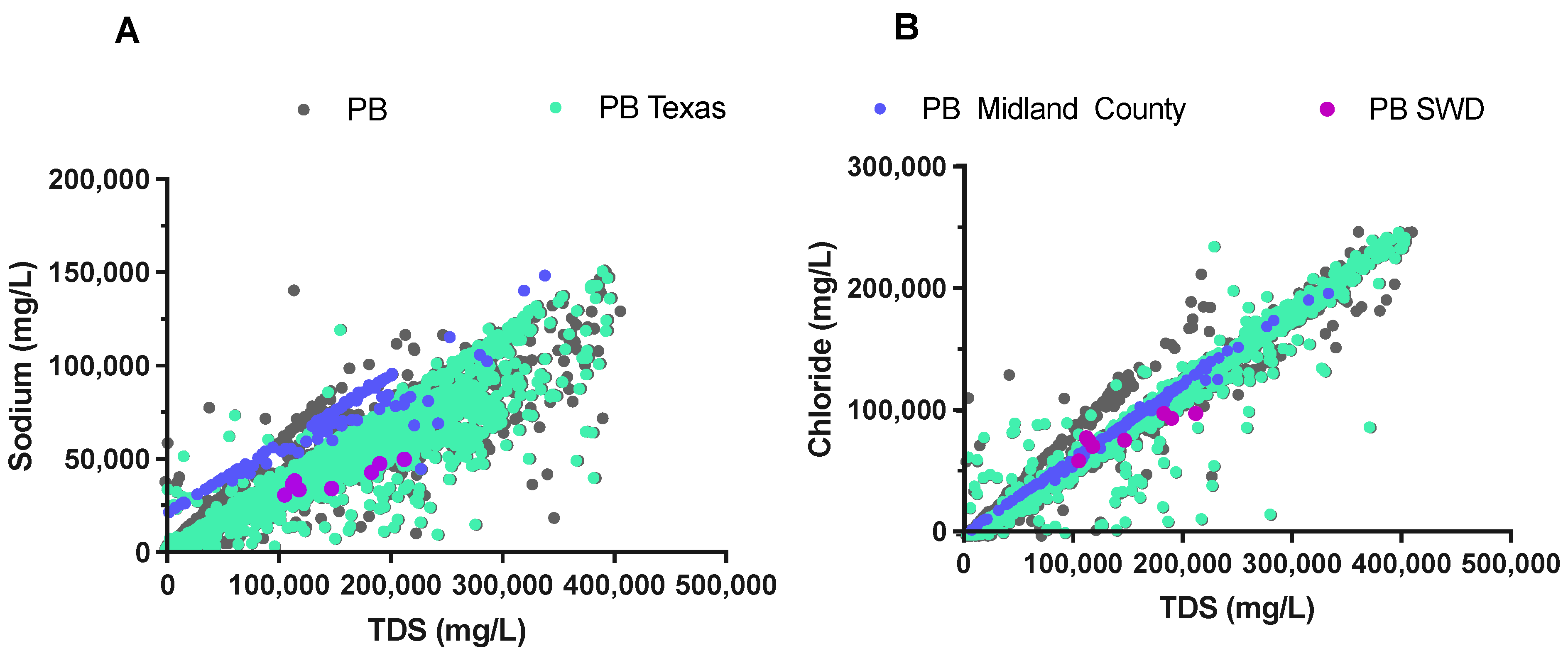
3.4. Permian Basin Salt Water Disposal Samples Compared to National Values

As previously mentioned, relatively few PW samples from UD have been analyzed compared to those from conventional development, in part due to difficulties in obtaining samples and to protect proprietary information. Therefore, an analysis was performed to compare PB SWD samples from UD with PW data from conventional oil and gas development reported by the USGS [50]. The principle behind the comparison was to determine if past samples could potentially be a predictor of the relative concentration of the PW of UD. Strong linear correlations were observed when comparing sodium and chloride ions found in sub-terrain water sources (Figure 8, r2-values 0.812–0.997, p-values < 0.0001–0.002). This is not surprising, given that sodium and chloride contribute a large majority of the dissolved solids found in the bulk measurement of TDS. Both sodium and chloride from PB SWD samples fell in line with the USGS’s data from conventional development in the PB.
The TDS levels detected in the PW samples collected from PB SWD are illustrated in Figure 9. This sample set was in the same range as other PB PW data gathered from the same county, which had an average concentration of 140,000 ± 60,000mg/L (Figure 9).
The most pertinent inorganic constituents, calcium and magnesium, are problematic due to their propensities to interact with carbonate and sulfate minerals [51]. Such interactions can be influenced by changes in temperature, pressure, pH, and salinity, as the water is brought to the surface and processed. The PB SWD magnesium levels were relatively low, even though calcium levels exceeded reuse limits. Despite what appeared to be elevated calcium concentrations, the values observed in the PB SWD samples fell below the mean of the reported Midland County values from conventional development [50]. This is represented in SI Figure S1.
Alkalinity and sulfate values observed in the PB SWD samples fell on the lower end of the PB spectrum reported by the USGS. The USGS PB dataset reported average values of 320 mg/L and 810 mg/L for alkalinity and sulfate, respectively. Alkalinity values for the PB SWD sample set were determined to be 162, 426, 204, 73.7, 841, 208, 622, and 515 mg/L (p = 0.0048). Sulfate values in the samples were 49.4, 33.1, 83.2, 77.1, 2.22, 416, 113, and 656 mg/L (p = 0.0658) (SI Table S3 and SI Figure S2).

3.5. Treatment Required for Direct Reuse and Beneficial Reuse

As previously mentioned, the reuse of PW for hydraulic fracturing depends on the depletion of predominantly inorganic ions. A good starting point for removing these scale-forming constituents (Ca, Mg, Ba, Si, and Sr) is the utilization of adsorbent materials, such as activated zeolite, alumina, and/or organoclays [52,53]). Electrocoagulation is a more sophisticated treatment that facilitates the reduction in ions, including the alkalizing species CO32− and HCO3−, based on their electrochemical properties [54,55]. Additionally, the implementation of membrane systems, such as reverse osmosis (RO) and forward osmosis (FO), is ideal for the removal of heavy metals [56]. Additionally, RO membranes can effectively remove B, which can affect the efficacy of crosslinkers in the HF fluid [57]. The beneficial reuse of purified PW in the agricultural sector requires stricter treatment to avoid harming crops. Advanced oxidation processes, such as photo-assisted and electrochemical processes, are candidates for the removal of radionuclides, heavy metals, and persistent toxic organic matter [58].). The integration of electrocoagulation and membrane technologies will ensure high-quality purified water with low salinity, TDS [59], as well as low concentration of harmful species that may affect crops.

4. Conclusions

It is inevitable that unconventional oil and gas practices will continue to grow to meet the growing energy demands of this nation [60]. There is an increasing need to facilitate the reuse and recycling of PW to mitigate the concerns related to induced seismic events and water usage. In this study, PB PW samples from UD were found to be comparable to the conventional PW samples. However, in general, PB PW samples from UD had ion concentrations measured to be on the lower end of the spectrum when compared to conventional PW samples from the same region. PW samples from two highly prolific shale basins in Texas regularly surpassed at least one of the reuse thresholds, indicating direct reuse of raw PW is not appropriate without some degree of treatment. More specifically, elevated levels of boron, calcium, and TSS could preclude raw PW from the PB region from being reused directly, whereas elevated levels of alkalinity, barium, boron, iron, and TSS would restrict the potential reuse of raw PW in the EF region. As has been observed in previous studies [5], the use of a single treatment modality is not sufficient when attempting to repurpose produced water, which is an inherently complex matrix that often contains undesirable constituents. Comprehensive treatment requires that a series of separation techniques/modalities be used in tandem, each of which targets specific constituents or classes of undesirable contaminants. For example, Isa et al. had a 97.6% efficiency when evaluating electrocoagulation for the removal of boron from PW [61]. Furthermore, nanofiltration has been successful in the removal of multivalent cations, such as calcium and magnesium [34]. Additionally, filtration, gravity separation, and coagulation are technologies used to reduce TSS [28]. System designs need to not only use diverse modalities to comprehensively treat PW, but they need to be inexpensive, modular in design, have a low tendency for fouling [8], provide significant throughput, and be able to desalinate the effluent or eliminate pertinent ions of concern.

Supplementary Materials

The following supporting information can be downloaded at: https://www.mdpi.com/article/10.3390/en15134521/s1, Figure S1: Histogram of the occurrence of concentration ranges for calcium and magnesium from 149 produced water samples collected from conventional production wells in Midland County, TX; Figure S2: Conventional hydrocarbon produced water data from 149 Midland County produced water samples; Table S1: Basic Produced Water Parameter; Table S2: Produced Water Metals; Table S3: Produced Water Anions; Table S4: Dilution factors used for analysis of metals in produced water solutions; Table S5: Percent recoveries and wavelengths used for metals in produced water solutions.

Author Contributions

Conceptualization, Z.L.H. and K.A.S.; methodology, T.L.; software, T.L.; validation, Z.L.H., K.A.S. and T.L.; formal analysis, T.L.; investigation, T.L.; resources, Z.L.H. and K.A.S.; data curation, T.L. and R.S.-R.; writing—original draft preparation, T.L.; writing—review and editing, Z.L.H., K.A.S. and R.S.-R.; visualization, T.L. and Z.L.H.; supervision, Z.L.H. and K.A.S.; project administration, Z.L.H. and K.A.S. All authors have read and agreed to the published version of the manuscript.

Funding

This research received no external funding.

Institutional Review Board Statement

Not applicable.

Informed Consent Statement

Not applicable.

Data Availability Statement

Not applicable.

Acknowledgments

Support for this work was provided by Asahi Kasei Corporation and the Collaborative Laboratories for Environmental Analysis and Remediation at the University of Texas, Arlington. We would also like to thank Challenger Water Solutions, the Apache Corporation, and Aris Water for supplying the produced water samples.

Conflicts of Interest

The authors declare no conflict of interest.

References

  1. Kim, S.; Omur-Ozbek, P.; Dhanasekar, A.; Prior, A.; Carlson, K. Temporal analysis of flowback and produced water composition from shale oil and gas operations: Impact of frac fluid characteristics. J. Pet. Sci. Eng. 2016, 147, 202–210. [Google Scholar] [CrossRef]
  2. Mobilia, M.; Comstock, O. U.S. Energy Consumption Rose Slightly in 2016 Despite a Significant Decline in Coal Use. 2017. Available online: https://www.ajot.com/news/u.s.-energy-consumption-rose-slightly-in-2016-despite-a-significant-decline (accessed on 19 April 2022).
  3. U.S. Energy Information Administration. Monthly Energy Review—April 2017; EIA: Washington, DC, USA, 2017.
  4. Liden, T.; Clark, B.G.; Hildenbrand, Z.L.; Schug, K.A. Unconventional Oil and Gas Production: Waste Management and the Water Cycle. In Environmental Issues Concerning Hydraulic Fracturing; Schug, K.A., Hildenbrand, Z.L., Eds.; APMP, Academic Press: Oxford, UK, 2017; Volume 1, pp. 17–45. [Google Scholar] [CrossRef]
  5. Hildenbrand, Z.L.; Santos, I.C.; Liden, T.; Carlton, D.D.; Varona-Torres, E.; Martin, M.S.; Reyes, M.L.; Mulla, S.R.; Schug, K.A. Characterizing variable biogeochemical changes during the treatment of produced oilfield waste. Sci. Total Environ. 2018, 634, 1519–1529. [Google Scholar] [CrossRef] [PubMed]
  6. Thacker, J.B.; Carlton, D.D., Jr.; Hildenbrand, Z.L.; Kadjo, A.; Schug, K.A. Chemical Analysis of Wastewater from Unconventional Drilling Operations. Water 2015, 7, 1568–1579. [Google Scholar] [CrossRef] [Green Version]
  7. Ground Water Protection Council, All Consulting. Modern Shale Gas—A Primer. 2009. Available online: https://www.energy.gov/fecm/downloads/modern-shale-gas-development-united-states-primer (accessed on 17 April 2022).
  8. Shaffer, D.; Chavez, L.H.A.; Ben-Sasson, M.; Castrillo, S.R.; Yin Yip, N.; Elimelech, M. Desalination and Reuse of High-Salinity Shale Gas Produced Water: Drivers, Technologies, and Future Directions. Environ. Sci. Technol. 2013, 47, 9569–9583. [Google Scholar] [CrossRef]
  9. Scanlon, B.R.; Reedy, R.C.; Xu, P.; Engle, M.; Nicot, J.P.; Yoxtheimer, D.; Yang, Q.; Ikonnikova, S. Can we beneficially reuse produced water from oil and gas extraction in the US? Sci. Total Environ. 2020, 717, 137085. [Google Scholar] [CrossRef]
  10. Nicot, J.P.; Scanlon, B.R.; Reedy, R.C.; Costley, R.A. Source and Fate of Hydraulic Fracturing Water in the Barnett Shale: A Historical Perspective. Environ. Sci. Technol. 2014, 48, 2464–2471. [Google Scholar] [CrossRef]
  11. Mantell, M. Produced Water Reuse and Recycling Challenges and Opportunities across Major Shale Plays. In EPA Hydraulic Fracturing Study Technical Workshop #4 Water Resources Management March; Chesapeake Energy Corporation: Oklahoma City, OK, USA, 2011; pp. 1–49. [Google Scholar]
  12. Ewing, B.T.; Waston, M.C.; McInturff, T.; McInturff, R. Economic Impact of the Permian Basin Oil and Gas Industry; Uddameri, V., Morse, A., Tindle, K.J., Eds.; CRC Press: Boca Raton, FL, USA, 2014; pp. 1–80. [Google Scholar]
  13. Scanlon, B.R.; Reedy, R.C.; Male, F.; Walsh, M. Water Issues Related to Transitioning from Conventional to Unconventional Oil Production in the Permian Basin. Environ. Sci. Technol. 2017, 51, 10903–10912. [Google Scholar] [CrossRef]
  14. Backstrom, J. Groundwater Regulations and Hydraulic Fracturing: Reporting Water Use in the Permian, College Station, TX, USA. 2018. Available online: https://agecograds.tamu.edu/wp-content/uploads/sites/49/2018/02/Groundwater-Regulations-and-Hydraulic-Fracturing-Reporting-Water-Use-in-Texas.pdf (accessed on 19 April 2022).
  15. Barclays, Columbia Water Center. The Water Challenge: Preserving a Global Resource. 2017. Available online: https://www.cib.barclays/content/dam/barclaysmicrosites/ibpublic/documents/our-insights/water-report/ImpactSeries_WaterReport_Final.pdf (accessed on 19 April 2022).
  16. Arthur, D.J.; Bohm, B.; Coughlin, B.J.; Layne, M.; Cornue, D. Evaluating the Environmental Implications of Hydraulic Fracturing in Shale Gas Reservoirs. In Proceedings of the SPE Americas E&P Environmental and Safety Conference, San Antonio, TX, USA, 23 March 2008; pp. 1–21. [Google Scholar] [CrossRef] [Green Version]
  17. Clark, C.E.; Veil, J.A. Produced Water Volumes and Management Practices in the United States; Argonne National Laboratory: Argonne, IL, USA, 2009. [CrossRef] [Green Version]
  18. Railroad Commission of Texas. Injection and Disposal Wells. 2017. Available online: http://www.rrc.state.tx.us/about-us/resource-center/faqs/oil-gas-faqs/faq-injection-and-disposal-wells/ (accessed on 7 July 2017).
  19. Van der Elst, N.J.; Page, M.T.; Weiser, D.A.; Goebel, T.H.W.; Hosseini, S.M. Induced earthquake magnitudes are as large as (statistically) expected. J. Geophys. Res. Solid Earth 2016, 121, 4575–4590. [Google Scholar] [CrossRef]
  20. Gallegos, T.J.; Varela, B.A.; Haines, S.S.; Engle, M.A. Hydraulic fracturing water use variability in the United States and potential environmental implications. Water Resour. Res. 2015, 51, 5839–5845. [Google Scholar] [CrossRef]
  21. Hornbach, M.J.; DeShon, H.R.; Ellsworth, W.L.; Stump, B.W.; Hayward, C.; Frohlich, C.; Oldham, H.R.; Olson, J.E.; Magnani, M.B.; Brokaw, C.; et al. Causal factors for seismicity near Azle, Texas. Nat. Commun. 2015, 6, 6728. [Google Scholar] [CrossRef] [Green Version]
  22. Hornbach, M.J.; Jones, M.; Scales, M.; DeShon, H.R.; Magnani, M.B.; Frohlich, C.; Stump, B.; Hayward, C.; Layton, M. Ellenburger wastewater injection and seismicity in North Texas. Phys. Earth Planet. Inter. 2016, 261, 54–68. [Google Scholar] [CrossRef] [Green Version]
  23. Magnani, M.B.; Blanpied, M.L.; DeShon, H.R.; Hornbach, M.J. Discriminating between natural versus induced seismicity from long-term deformation history of intraplate faults. Sci. Adv. 2017, 3, e1701593. [Google Scholar] [CrossRef] [PubMed] [Green Version]
  24. Wang, Q.; Chen, X.; Jha, A.N.; Rogers, H. Natural gas from shale formation-The evolution, evidence, and challenges of shale gas revolution in United States. Renew. Sustain. Energy Rev. 2014, 30, 1–28. [Google Scholar] [CrossRef]
  25. Jula, M. In Oklahoma, Injecting Less Saltwater Lowers Quake Rates. Sci. Magzine 2016, 2016–2019. Available online: https://www.aaas.org/news/oklahoma-injecting-less-saltwater-lowers-quake-rates (accessed on 19 April 2022).
  26. Parker, K.M.; Zeng, T.; Harkness, J.; Vengosh, A.; Mitch, W.A. Enhanced formation of disinfection byproducts in shale gas wastewater-impacted drinking water supplies. Environ. Sci. Technol. 2014, 48, 11161–11169. [Google Scholar] [CrossRef]
  27. King, G.E. Treating Produced Water for Shale Fracs; Society of Petroleum Engineers Gulf Coast Section: Houston, TX, USA, 2011; pp. 1–20. [Google Scholar]
  28. Liden, T.; Santos, I.C.; Hildenbrand, Z.L.; Schug, K.A. Treatment Modalities for the Reuse of Produced Waste from Oil and Gas Development. Sci. Total Environ. 2018, 643, 107–118. [Google Scholar] [CrossRef]
  29. Oetjen, K.; Chan, K.E.; Gulmark, K.; Christensen, J.H.; Blotevogel, J.; Borch, T.; Spear, J.R.; Cath, T.Y.; Higgins, C.P. Temporal characterization and statistical analysis of flowback and produced waters and their potential for reuse. Sci. Total Environ. 2018, 619–620, 654–664. [Google Scholar] [CrossRef]
  30. Hildenbrand, Z.L.; Carlton, D.D., Jr.; Fontenot, B.E.; Meik, J.M.; Walton, J.L.; Taylor, J.T.; Thacker, J.B.; Korlie, S.; Shelor, C.P.; Henderson, D.; et al. A Comprehensive Analysis of Groundwater Quality in The Barnett Shale Region. Environ. Sci. Technol. 2015, 49, 8254–8262. [Google Scholar] [CrossRef] [Green Version]
  31. Hildenbrand, Z.L.; Carlton, D.D., Jr.; Fontenot, B.E.; Meik, J.M.; Walton, J.L.; Thacker, J.B.; Korlie, S.; Shelor, C.P.; Kadjo, A.F.; Clark, A.; et al. Temporal variation in groundwater quality in the Permian Basin of Texas, a region of increasing unconventional oil and gas development. Sci. Total Environ. 2016, 562, 906–913. [Google Scholar] [CrossRef]
  32. Otton, J.K.; Mercier, T. Produced Water Brine and Stream Salinity, U.S. Geological Survey. Available online: https://water.usgs.gov/orh/nrwww/Otten.pdf (accessed on 19 April 2022).
  33. Wasylishen, R.; Fulton, S. Reuse of Flowback & Produced Water for Hydraulic Fracturing in Tight Oil. Calgary 2012, 34. Available online: https://hero.epa.gov/hero/index.cfm/reference/details/reference_id/2828355 (accessed on 19 April 2022).
  34. Ahmadun, F.-R.; Pendashteh, A.; Abdullah, L.C.; Biak, D.R.A.; Madaeni, S.S.; Abidin, Z.Z. Review of technologies for oil and gas produced water treatment. J. Hazard. Mater. 2009, 170, 530–551. [Google Scholar] [CrossRef]
  35. Hu, Y.; Mackay, E.; Ishkov, O.; Strachan, A. Predicted and Observed Evolution of Produced-Brine Compositions and Implications for Scale Management. SPE Prod. Oper. 2016, 31, 270–279. [Google Scholar] [CrossRef]
  36. Moghadasi, J.; Muller-Steinhagen, H.; Jamaialahmadi, M.; Sharif, A. Prediction of Scale Formation Problems in Oil Reservoirs and Production Equipment due to Injection of Incompatible Waters. Asia-Pac. J. Chem. Eng. 2006, 14, 545–566. [Google Scholar] [CrossRef]
  37. Lunevich, L.; Sanciolo, P.; Milne, N.; Gray, S.R. Silica Fouling in Coal Seam Gas Water Reverse Osmosis Desalination. Environ. Sci. Water Res. Technol. 2017, 3, 911–921. [Google Scholar] [CrossRef]
  38. Montgomery, C. Fracturing Fluid Components. In Effective and Sustainable Hydraulic Fracturing; Jeffrey, R., Ed.; Intech: Oxford, UK, 2013; pp. 25–45. [Google Scholar] [CrossRef] [Green Version]
  39. Esmaeilirad, N.; White, S.; Terry, C.; Prior, A.; Carlson, K. Influence of inorganic ions in recycled produced water on gel-based hydraulic fracturing fluid viscosity. J. Pet. Sci. Eng. 2016, 139, 104–111. [Google Scholar] [CrossRef]
  40. Fink, J.K. Water-Based Chemicals and Technology for Drilling, Completion, and Workover Fluids. In Water-Based Chemicals and Technology for Drilling, Completion, and Workover Fluids; Gulf Professional Publishing: Boston, MA, USA, 2015; pp. i–ii. [Google Scholar] [CrossRef]
  41. Gulbis, J.; Hodge, R.M. Fracturing Fluid Chemistry and Proppants; Economides, M.J., Boney, C., Eds.; Reservoir Stimulation: New York, NY, USA, 2000; p. 856. [Google Scholar] [CrossRef]
  42. King, G.E.; Durham, D. Chemicals in Drilling, Stimulation, and Production. In Environmental Issues Concerning Hydraulic Fracturing; Schug, K.A., Hildenbrand, Z.L., Eds.; APMP, Academic Press: Oxford, UK, 2017; Volume 1, pp. 47–63. [Google Scholar]
  43. U.S. Environmental Protection Agency. Evaluation of Impacts to Underground Sources of Drinking Water by Hydraulic Fracturing of Coalbed Methane Reservoirs; John Wiley & Sons: Hoboken, NJ, USA, 2004. [CrossRef]
  44. Jennings, H.; Muroski, F. Removal of Hydrogen Sulfide with Potassium Permanganate. Am. Water Work. Assoc. 1964, 56, 475–479. [Google Scholar]
  45. Chang, C.-Y.; Hsieh, Y.-H.; Hsu, S.-S.; Hu, P.-Y.; Wang, K.-H. The formation of disinfection by-products in water treated with chlorine dioxide. J. Hazard. Mater. 2000, 79, 89–102. [Google Scholar] [CrossRef]
  46. Hua, G.; Reckhow, D.A.; Kim, J. Effect of Bromide and Iodide Ions on the Formation and Speciation of Disinfection Byproducts during Chlorination. Environ. Sci. Technol. 2006, 40, 3050–3056. [Google Scholar] [CrossRef]
  47. Vashishtha, D.; Villalobos, J.; Jimenez, D. Use of Chemicals in Disinfection: Implications and Alternatives. Ind. Water World 2017. Available online: https://www.watertechonline.com/wastewater/article/16210939/use-of-chemicals-in-disinfection-implications-and-alternatives (accessed on 18 April 2022).
  48. Symons, J.M.; Krasner, S.W.; Simms, L.A.; Sclimenti, M. Measurement of THM and Precursor Concentrations Revisited: The Effect of Bromide Ion. J. Am. Water Works Assoc. 1993, 85, 51–62. [Google Scholar] [CrossRef]
  49. Murali Mohan, A.; Hartsock, A.; Bibby, K.J.; Hammack, R.W.; Vidic, R.D.; Gregory, K.B. Microbial Community Changes in Hydraulic Fracturing Fluids and Produced Water from Shale Gas Extraction. Environ. Sci. Technol. 2013, 47, 13141–13150. [Google Scholar] [CrossRef]
  50. Blondes, M.S.; Gans, K.D.; Rowan, E.L.; Thordsen, J.J.; Reidy, M.E.; Engle, M.A.; Kharaka, Y.K.; Thomas, B. U.S. Geological Survey National Produced Waters Geochemical Database. 2017. Available online: https://energy.usgs.gov/EnvironmentalAspects/EnvironmentalAspectsofEnergyProductionandUse/ProducedWaters.aspx#3822349-data (accessed on 1 January 2016).
  51. Zielinski, R.A.; Otton, J.K. Naturally Occurring Radioactive Materials (NORM) in Produced Water and Oil-Field Equipment—An Issue for the Energy Industry. 1999. Available online: https://pubs.usgs.gov/fs/fs-0142-99/fs-0142-99.pdf (accessed on 17 April 2022).
  52. Chang, H.; Liu, T.; He, Q.; Li, D.; Crittenden, J.; Liu, B. Removal of calcium and magnesium ions from shale gas flowback water by chemically activated zeolite. Water Sci. Technol. 2017, 76, 575–583. [Google Scholar] [CrossRef] [PubMed] [Green Version]
  53. Igunnu, E.T.; Chen, G.Z. Produced water treatment technologies. Int. J. Low Carbon Technol. 2014, 9, 157–177. [Google Scholar] [CrossRef] [Green Version]
  54. Kausley, S.B.; Malhotra, C.P.; Pandit, A.B. Treatment and reuse of shale gas wastewater: Electrocoagulation system for enhanced removal of organic contamination and scale causing divalent cations. J. Water Process Eng. 2017, 16, 149–162. [Google Scholar] [CrossRef]
  55. Khor, C.M.; Wang, J.; Li, M.; Oettel, B.A.; Kaner, R.B.; Jassby, D.; Hoek, E.M.V. Performance, energy and cost of produced water treatment by chemical and electrochemical coagulation. Water 2020, 12, 3426. [Google Scholar] [CrossRef]
  56. Cui, Y.; Ge, Q.; Liu, X.Y.; Chung, T.S. Novel forward osmosis process to effectively remove heavy metal ions. J. Membr. Sci. 2014, 467, 188–194. [Google Scholar] [CrossRef]
  57. Li, Y.; Wang, S.; Song, X.; Zhou, Y.; Shen, H.; Cao, X.; Zhang, P.; Gao, C. High boron removal polyamide reverse osmosis membranes by swelling induced embedding of a sulfonyl molecular plug. J. Membr. Sci. 2020, 597, 117716. [Google Scholar] [CrossRef]
  58. Coha, M.; Farinelli, G.; Tiraferri, A.; Minella, M.; Vione, D. Advanced oxidation processes in the removal of organic substances from produced water: Potential, configurations, and research needs. Chem. Eng. J. 2021, 414, 128668. [Google Scholar] [CrossRef]
  59. Zhao, S.; Hu, S.; Zhang, X.; Song, L.; Wang, Y.; Tan, M.; Kong, L.; Zhang, Y. Integrated membrane system without adding chemicals for produced water desalination towards zero liquid discharge. Desalination 2020, 496, 114693. [Google Scholar] [CrossRef]
  60. U.S. Department of Energy. Advancing Systems and Technologies to Produce Cleaner Fuels Technology Assessments: Unconventional Oil and Gas, Quadrennial Technology Review 2015; United State Department of Energy: Washington, DC, USA, 2015.
  61. Isa, M.H.; Ezechi, E.H.; Ahmed, Z.; Magram, S.F.; Kutty, S.R.M. Boron removal by electrocoagulation and recovery. Water Res. 2014, 51, 113–123. [Google Scholar] [CrossRef]
Figure 1. Sampling locations for the produced water samples in this study. Nine were collected from the Permian Basin: one considered FB from Nolan County, TX, one from a SWD well in Dawson County TX, and seven from a SWD in Midland County, TX. In total, 15 samples were collected from the Eagle Ford Shale: 13 from a PW treatment center in Bebe, TX, and two from EF production wells in Brazos County, TX.
Energies 15 04521 g001
Figure 2. The collective (A) TDS and (B) TSS of the samples from different regions. The mean values are graphed with error bars illustrating standard error of the mean. The dashed lines represent recommended water quality guidelines for the reuse of PW for production well stimulation, as authored by Hildenbrand, King, Oetjen, and Liden et al. [5,27,28,29].
Energies 15 04521 g002
Figure 3. The analysis of (A) alkalinity, (B) pH, and (C) TOC in the various PW samples. Data are presented as mean values with the error bars representing standard error of the mean. The dashed lines represent recommended levels for the reuse of PW for production well stimulation authored by Hildenbrand, King, Oetjen, and Liden et al. [5,27,28,29].
Energies 15 04521 g003
Figure 4. Scaling contributors for each PW sample set, including Permian Basin flowback, Permian Basin SWD, EF treatment facility, and EF production wells, all represented in the graphs. Data are presented as mean values for (A) barium, (B) calcium, (C) magnesium, (D) strontium, and (E) silicon with the error bars representing standard error of the mean. Dotted lines mark the recommended maximum reuse limit suggested by Hildenbrand, King, Oetjen, and Liden et al. [5,27,28,29].
Energies 15 04521 g004
Figure 5. Boron (A) and iron (B) concentrations for the PW sample set. Data are presented as mean values with the error bars representing standard error of the mean. The reuse limits recommended by Hildenbrand, King, Oetjen, and Liden et al. are represented with black dotted lines [5,27,28,29].
Energies 15 04521 g005
Figure 6. Metals in produced waters that primarily contribute to TDS levels. The average concentrations for (A) sodium, (B) potassium, (C) lithium, and (D) manganese are presented, along with error bars, which represent the standard error of the mean.
Energies 15 04521 g006
Figure 7. Average anion concentrations found in the PW samples sets for (A) bromide, (B) chloride, (C) fluoride, (D) nitrate, and (E) sulfate. The reuse limits recommended by Hildenbrand, King, Oetjen, and Liden et al. are represented by black dotted lines. The error bars represent the standard error of the mean [5,27,28,29].
Energies 15 04521 g007
Figure 8. Correlation of (A) sodium and (B) chloride concentrations with TDS levels, plotted from conventional well PW data reported by the USGS for the PB (gray), Texas-based PB wells (cyan), production wells located in Midland County (purple), as well as the values measured for PW from UD-labeled PB SWD (magenta). The USGS’s dataset for the Permian Basin data included 16,000 samples from conventional oil and gas operations [50].
Energies 15 04521 g008
Figure 9. Histogram of TDS concentrations from PB data reported by the USGS for wells located in Midland County [50]. The data illustrate the concentrations stated for conventional wells. The graph inset in the top right corner represents the conventional waste range and the average of 149 Midland County PW data points. The black lines denote individual TDS values from the PB SWD sample set.
Energies 15 04521 g009
Table 1. Maximum contaminant limits for production well stimulation fluid [5,27,29].
Production Well Stimulation (mg/L)Production Concern
pH6.5–8.5Corrosion/Scaling
TSS500
Chloride30,000–50,000Fluid instability
Sulfate500Scaling/Bacterial substrate
Bicarbonate300Scaling
Silica35Scaling
Boron (B)10Crosslinker efficiency
Barium (Ba)20Scaling
Calcium (Ca)2000Scaling
Iron (Fe)10Crosslinker efficiency
Magnesium (Mg)2000Scaling
Publisher’s Note: MDPI stays neutral with regard to jurisdictional claims in published maps and institutional affiliations.

