Energy Assessment of the Thermal Bridging Effects on Different Structural Envelope Types Using Mixed-Equivalent-Wall Method

Abstract

In this paper, the effect of house envelopes including thermal bridges on the daily, monthly, and annual consumption of the air conditioning system of a detached house and an attached house, with a façade in the east, west, north, or south direction, is investigated; moreover, the capacity of the air conditioning system is calculated for detached and attached houses based on the maximum hourly peak load during severe weather conditions. The four tested house envelopes are exterior insulation and finish system (EIFS), autoclaved aerated concrete block (AAC-B), classical (cement blocks with insulation in between), and AAC column and beam (AAC-CB). The work is conducted using a method that combines the finite element method (COMSOL Multiphysics), building simulation (EnergyPlus), and the Engineering Equation Solver (EES) programs. The results indicated that the annual consumption of the air conditioning system using AAC-B, classical, and AAC-CB envelopes is larger than that of EIFS by about 3.74, 11.53, and 20.70% for the detached house, and 1.8, 2.9%, and 6.7% for the attached house, respectively. The annual consumption of the air conditioner of the detached house is larger than the average consumption of the attached house by about 25.3, 27.7, 35.8, and 41.7% for EIFS, AAC-B, classical, and AAC-CB house envelopes, respectively. Using the different façade directions of the attached house, the average effect of the house envelope type on the air conditioning system capacity is about 8.84%, with a standard deviation of 0.466%.

1. Introduction

On the global level, buildings are claimed to be responsible for 40% of the energy required and 30% of CO₂ emissions [1]. The energy usage in the residential building sector in hot climate countries is over 70%, where most of which is due to air conditioning consumption [2]. The building envelope plays a pivotal role in controlling heat transmissions between the building and the outside environment [3,4,5]. Thus, enhancement of the building envelope performance is a central issue that needs to be accomplished by engineers and designers. Increasing the insulation thickness is an effective measure to improve the thermal performance of the building envelope; however, unintentionally a significant part of heat losses bypasses the insulation layer through discontinuous insulated layers of what is known as thermal bridges (TBs). The TBs are formed in the building envelope, when two elements of different materials are combined, such as the joint between the roof or floor slab and the external wall. The discontinuous portion of an exterior wall can correspond to 50–80% of the wall area [6,7]. Many codes and standards [8] proposed a procedure to account for TBs influence, but most of them used simplified methods to encounter the TBs effect.

In a similar approach, the building energy simulation program (BESP) which is used to assess the building thermal performance, tends to use a one-dimensional (1-D) model to describe the thermal behavior of the building envelope elements [9]. If the obtained equivalent wall does not have the same dynamic behavior as the thermal bridge, such an approach calculates the heat transmission due to the thermal bridges but will dismiss the dynamic aspect of it, i.e., the time lag [10]. Thermal bridging requires more accurate of two- or three-dimensional models to account for these effects, which influence the energy demand of dwellings between 5 and 39% [11].

A practical method that can represent the thermal bridge’s real behavior and can be integrated with BSP introduces the equivalent wall (EqW) method. The EqW method involves creating a fictitious 3-layer wall with selected properties; its dynamic response to the transient conditions is the same as the real wall with two- and three-dimensional effects [7]. EqW method has been evolved and implemented by several approaches, such as the structure factors method [12,13], the matrix of transfer functions method [14], the harmonic method [15,16], and an identification method [17]. The widely accepted and used methods are structure factors and harmonic; however, they are not functioning adequality; the former gives infinite solutions (no unique solution), while the latter has less accuracy [18]. A new method that mixes the structure factors and the harmonic methods to utilize their strength and overcome their limitations to a more efficient method is introduced, mixed method (MM) [19]. The MM considers the stationary, dynamic, and harmonic phenomena of a thermal bridge and obtains more efficient results. It showed a 0.9% difference in the equivalent wall (1-D 3-layer) heat flux compared to the real structure wall [20].

The previous work analyzed the effect of the TB bypassing the insulation layers of double block [21], but less considered the rapid spread of Autoclaved Aerated Concrete (AAC) block [22]. Construction firms prefer AAC due to the advantages of lightweight and high thermal performance. Thus, the AAC block becomes one of the primary materials for constructing self-insulation exterior walls in recent years. It is treated as the preferred filling material of a frame structure of medium to high-rise residential and commercial buildings; it is also used in the load-bearing exterior wall of low-rise residential buildings; however, the AAC walls are surrounded by a commonly built frame from a highly conductive material such as reinforced concrete, which increases the thermal bridge’s influence (TB).

To the best knowledge of the authors, the combined effect of the exterior wall type and thermal bridge on the energy consumption of buildings is not reported in the open literature. With the exception of this, the research team of the present paper has investigated the thermal characteristics of four heavy structure residential building envelopes in hot climates, including the effect of thermal bridges (Al-Awadi et al. [23]); they concluded that the thermal bridges have a more considerable effect on some wall types, such as the classical (cement block with intermediate insulation) and autoclaved aerated concrete wall with columns and beams (AAC-CB), than others such as exterior insulation and finish system (EIFS) and autoclaved aerated concrete block without columns in the structure (AAC). The authors focused on the heat transmission with the outdoor environment and reported that houses made using a specific wall type exchange only half the heat exchanged by another type; this was due to the combined effect of wall type and thermal bridges effect. Al-Awadi et al. [23] recommended extending their study to include the effects of façade orientation and actual solar radiation on the capacity and energy consumption of air conditioning systems in hot climates.

Therefore, this paper is considered part two of the above-stated paper [23] to extend the work from thermal characteristics to the energy consumption of buildings; it includes the effects of wall type, façade orientation, and solar insolation on the capacity and consumption of air conditioning systems used in attached and detached houses in hot climate countries. The external wall of the tested houses is structured using four types, considering the thermal bridges at the junctions between the concrete roof and floor slabs of each floor, with the external walls, and between walls and concrete columns. The four considered envelopes are made of EIFS, AAC-B, classical, and AAC-CB. Therefore, the present paper combined the effects of external wall types and thermal bridges on the energy consumption of air conditioning systems of detached and attached houses. To account for thermal bridges, a robust equivalent wall method, mix-method (MM), is implemented to evaluate both heat flow and time lag (phase shift) of the thermal bridge (TB).

2. Materials and Methods

2.1. Materials

The considered house is in the State of Kuwait which is a hot climate country; it consists of three floors, each is 20 × 20 m² area and 4 m high. Two house cases are considered where the first is when all house sides are exposed to external conditions (detached house), while the second case has one wall side exposed to external conditions and the other three sides are attached to neighboring buildings (attached house). The building’s opaque envelope consists of walls, roof, beams, and slab-on-grade. The envelope is the main building component that holds its structural elements and prevents the outside condition from an immediate effect on the inside condition; however, the external surfaces (wall, roof, slab-on-grade) are attached with different mechanisms, all of which do not totally ensure continuity of the insulation material, and this creates a material discontinuity that causes what is known as thermal bridges (TBs).

The attached and detached house envelopes are shown in Figure 1, illustrating the tested thermal bridges: at the roof-wall junction (yellow), intermediate slab-wall junctions (purple), the slab-on-grade-wall junction (red), and columns-wall junctions (green). The combined effect of the thermal bridges and the external wall types of the attached and detached house envelopes is investigated. The considered wall types are the exterior insulation and finish system (EIFS), autoclaved aerated concrete (AAC) block without concrete columns (AAC-B), classical cement blocks with intermediate insulation (classical), and AAC supported by columns and beams (AAC-CB).

Table 1. Physical properties of residential building construction materials.

Construction	mc/A	Rtotal	U	a × 107
	kJ/Km2	m2 K/W	W/m2 K	m2/s
Concrete Slabs:
Slab-on-Grade	450.45	0.13	7.83	10.00
Intermediate Floor slab	465.45	0.12	8.16	10.001
Roof slab	511.35	2.34	0.43	7.827
Concrete Columns	1200.0	0.20	5.00	10.40
External Walls:
EIFS	293.58	1.76	0.568	7.236
AAC-Bearing (AAC-B)	168.77	1.88	0.53	3.223
Classical	368.69	1.86	0.54	4.981
AAC Colm. Beam (AAC-CB)	168.77	1.23	0.82	3.985

gives the physical properties of the examined wall types and the various concrete slabs.

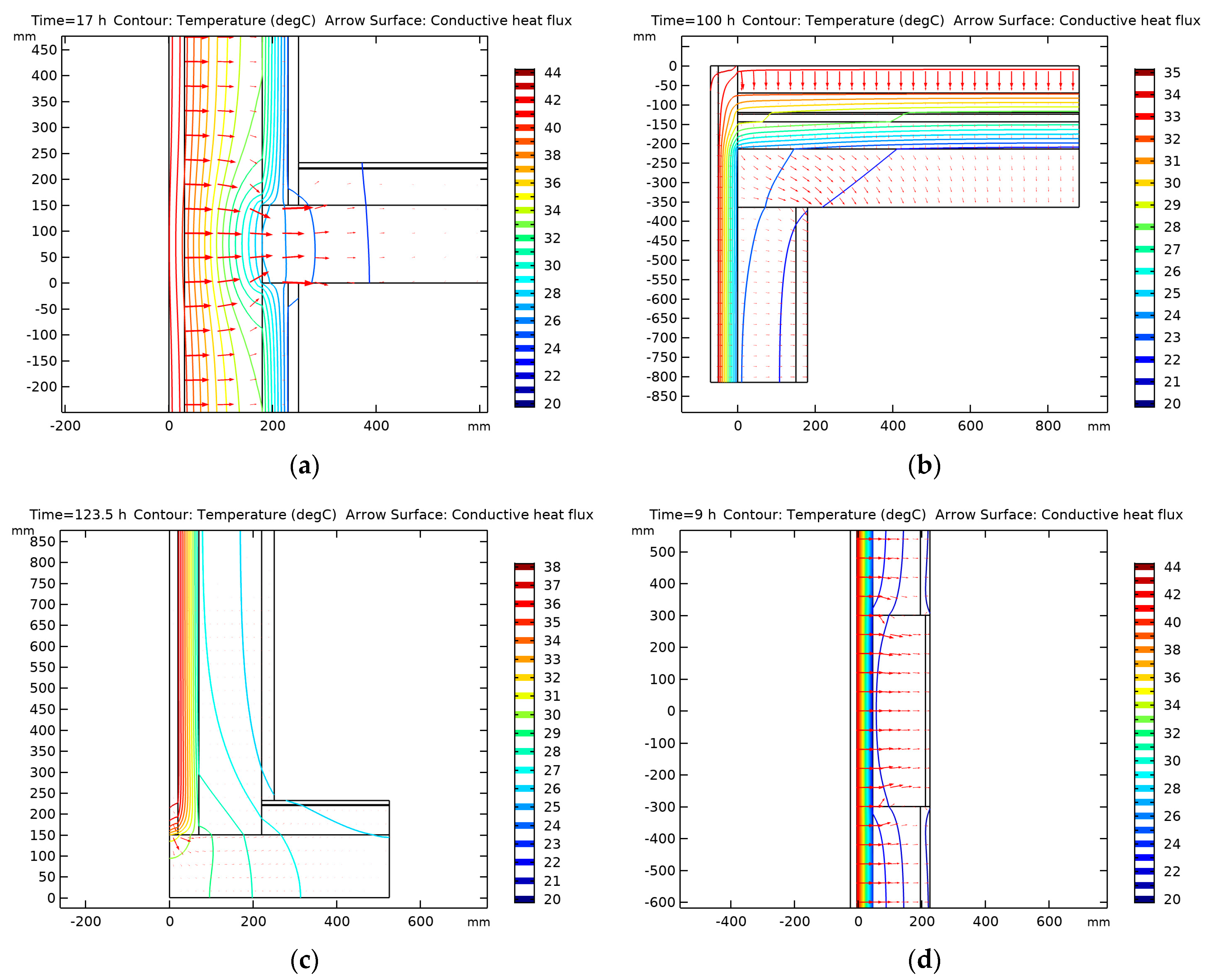
2.2. Studied Thermal Bridge Cases

The initial step in evaluating the real effect of the thermal bridge on building envelopes is to model the case using multi-physics software such as COMSOL. As shown in Figure 2, the discontinuous junction between the external wall and roof, intermediate floor, and slab-on-grade are driving the heat flow, from the higher temperature toward the lower, in a more complex pattern. A detailed analysis of the thermal bridge effect of the studied wall types was introduced by the same authors in a previous study [23].

In this study, an equivalent wall of three layers (1−D) that behaves similarly to the actual 2−D wall, including the thermal bridge, is to be determined. Such findings will ease and ensure the high accuracy of the thermal bridge that can be used in a Building Energy Simulation Program (BESP). The procedures for finding the equivalent wall will be discussed in the next section.

It is worth noting that the employed 2−D heat transmission analysis software (COMSOL) is designed to solve the problem using the finite element method.

Precise CFD (Computational Fluid Dynamics) results need a refined mesh to obtain results that are independent of the size of the mesh. Hence, the considered thermal bridge is modeled and meshed with four sizes. Namely, coarse, normal, fine, and finer mesh settings with 6629, 7506, 7674, and 8997 elements, respectively. Those mesh sizes are created automatically by the program and tested to choose the mesh that provides a converged solution, accurate results, and a suitable computational time. The computed temperature and heat flux inside the thermal bridge using the tested mesh sizes with the percentage difference between the values computed by each mesh and the finer one is listed in

Table 2. Mesh sensitivity analysis for a thermal bridge sample.

Mesh Type (# Elements)	Coarse (6629)	Normal (7506)	Fine (7674)	Finer (8997)
Tin (°C)	0.082459	0.082451	0.082450	0.082447
%Difference	0.014555	0.004852	0.003639	0.0
qin (W/m2)	0.68169	0.68169	0.68160	0.68162
%Difference	0.01027	0.01027	0.002934	0.0

. In general, the difference between the computed value by each mesh and the finer one reduces as the mesh size increases. The difference in stationary temperature and heat flux is lower than 0.01% between the fine and finer meshes. Thus, the sensitivity analysis confirmed the accurate results of the simulations and their independence on mesh size using the fine-size mesh.

2.3. Implementation of Mixed-Equivalent-Wall Method (MEWM)

The equivalent wall method idea is to substitute the real 2−D or 3−D thermal bridge with a simple 1−D multilayer wall of the same dynamic and static thermal performances. The equivalent wall characteristics involve finding the thermal resistance R_m and the heat capacity C_m of each layer m. Carpenter [13] and Martin et al. [20] reported that three layers are optimal to configure the equivalent wall. Using more layers might lead to an accurate structure, however, their determination requires greater computational efforts.

There were many methods to acquire the properties of the equivalent wall, i.e., the structure factors, matrix of transfer functions, harmonic, and identification methods; however, the mixed method between harmonic and structure factors introduced by Quinten and Feldheim [24] develop a simple, accurate and original method to consider the real thermal bridges effects and incorporate it into a building energy simulation program which is explained in the following steps:

Step 0: Initial inputs and assumptions

• Imposing the same thickness of the three wall layers (e_m = e/3) and each layer with a density of ρ_m = 1000 kg/m³. The values of the thermal conductivity and the specific heat capacity of each layer of the equivalent wall are deduced from the values of total calculated thermal resistance (R_m) and thermal capacitance (C_m).
• The area of influence of the thermal bridge, to be replaced by the equivalent structure, must be limited by adiabatic cut−off planes. Thus, in all cases, a first steady−state simulation is needed to locate those adiabatic surfaces.
• For the three-layer wall, six parameters (R₁, R₂, R₃, C₁, C₂, and C₃) are required to be determined; this can be obtained by finding the five numbers characterizing the thermal behavior of the wall, namely, the overall resistance R, the overall capacity C, and the three structure factors (${\varnothing }_{ii}$, ${\varnothing }_{ie}$, and ${\varnothing }_{ee}$).
• The inside and outside air resistances are found by fixed values, R_i = 1/h_i = 1/8, R_e = 1/h_e = 1/23, (m² K/W).

Step 1: Locate the adiabatic cut-off planes of the 2-D detail

• The cut-off planes define the computational domain of the thermal bridge to study. The cut-off planes are considered to be adiabatic if they are far from the 2-D heat flow. They are first placed at one meter from the 2−D/3−D detail (EN ISO 10211) except if there is a closer adiabatic plane [25].
• A steady−state simulation is executed with (T_e = 0 °C, T_i = 20 °C). The inner/outer surface temperatures (T_si and T_se) are examined for deviations smaller than 0.01 °C at the extended boundaries to alcoate new cut-off planes; this will avoid unnecessary additional calculations to the model and focus the study on the behavior of the thermal bridge.

Step 2: Thermal properties of the thermal bridge

The structure factors $\varnothing$ are computed using Equations (1)–(3) and the heat capacity C using Equation (4) The thermal resistance R is deduced from the value of the heat flux through the inner (q_i) or outer (q_o) surface R = 1/|q_i| = 1/|q_e| in steady-state when |T_e − T_i| = 1K with q in W/m² or W/m.

$${\varnothing }_{ii}=\frac{1}{C}{{\displaystyle \int }}_V^{}\rho c{\left(1-T\left(x,y,z\right)\right)}^{2}dV$$

(1)

$${\varnothing }_{ie}=\frac{1}{C}{{\displaystyle \int }}_V^{}\rho c\left(T\left(x,y,z\right)\right)\left(1-T\left(x,y,z\right)\right)dV$$

(2)

$${\varnothing }_{ee}=\frac{1}{C}{{\displaystyle \int }}_V^{}\rho c{\left(T\left(x,y,z\right)\right)}^{2}dV$$

(3)

$$C=\underset{V}{\overset{}{{\displaystyle \int }}}\rho c dV$$

(4)

A dynamic simulation is performed for at least 10 days with T_e = sin (2 π t/86,400), T_i = 0 °C. According to Quinten and Feldheim [24], the results are not affected by the initial conditions; therefore, the results were analyzed after seven days (168 h). From the simulation results, the heat flux amplitude (W/m²) and phase shift of the temperature through the inner and outer surfaces are deduced, A_i (24 h) and A_e (24 h), α_i (24 h) and α_e (24 h), respectively.

Step 3: Finding the 1-D three-layer equivalent wall (EES program)

A reference surface area S_ref (m or m²) is usually the projected external surface area of the initial wall. To ensure the heat flux balance, the convection heat transfer coefficients h* for the equivalent adapted as in Equations (5) and (6).

h_e,in × S_e = h^*_{e, eq} × S_ref

(5)

h_i,in × S_e = h^*_{i, eq} × S_ref

(6)

A simple way to solve for equivalent layer properties is to first generate initial values with some logic, a set of capacitances C_m (or resistances R_m) for each layer, then seek the resistances R_m (or capacitances C_m) to satisfy the below Equations (7)–(11).

The thermal structure factors and overall R-value must match those for the 3-D wall assembly. The thermo–physical properties of the layers may then be established, if necessary, to match R_m and C_m values and the total thickness of the wall. Different combinations of R₂ and R₃ are tested, and discrete values are used.

For each combination of R₂ and R₃, R₁, C₁, C₂, and C₃ are determined to guarantee the same values of structure factors, heat capacity, and thermal resistance as for the 2-D/3-D thermal bridge using Equations (7) and (9)–(11).

$${\varnothing }_{ii}=\frac{1}{R^2\ast C} \ast \left(\begin{array}{c}{C}_1\ast \left(\frac{R_1{}^2}{3}+R_1\ast \left(R_2+R_3+R_e\right)+{\left(R_2+R_3+R_e\right)}^2\right)\\ +C_2\ast \left(\frac{R_2{}^2}{3}+R_2\ast \left(R_3+R_e\right)+{\left(R_3+R_e\right)}^2\right)\\ +C_3\ast \left(\frac{R_3{}^2}{3}+R_3\ast R_e+R_e{}^2\right)\end{array}\right)$$

(7)

$${\varnothing }_{ie}=\frac{1}{R^2\ast C}\ast \left(\begin{array}{c}{C}_1\ast \left(\frac{R_1^2}{3}+\left(R_1\ast R_i\right)+R_i^2\right)\\ +C_2\ast \left(\frac{R_2^2}{3}+R_2\ast \left(R_i+R_1\right)+{\left(R_i+R_1\right)}^2\right)\\ +C_3\ast \left(\frac{R_3^2}{3}+R_3\ast \left(R_i+R_1+R_2\right)+{\left(R_i+R_1+R_2\right)}^2\right)\end{array}\right)$$

(8)

$${\varnothing }_{ee}=\frac{1}{R^2\ast C}\ast \left(\begin{array}{c}{C}_1\ast \left(-\frac{R_1^2}{3}+\frac{R_1\ast R}{2}+R_i\ast \left(R_2+R_3+R_e\right)\right)\\ +C_2\ast \left(-\frac{R_2^2}{3}+\frac{R_2\ast R}{2}+\left(R_i+R_1\right)\ast \left(R_3+R_e\right)\right)\\ +C_3\ast \left(-\frac{R_3^2}{3}+\frac{R_3\ast R}{2}+\left(R_i+R_1+R_2\right)\ast R_e\right)\end{array}\right)$$

(9)

$$R=R_1+R_2+R_3+R_{i,eq}+R_{e,eq}$$

(10)

$$C=C_1+C_2+C_3$$

(11)

Step 4: Iterating process to find the equivalent wall characteristic (EES script)

Many combinations can be achieved using the above method. Therefore, values of the C_n and R_n are achieved within certain constraints, where if not met, the results are ignored and disregarded from the set. Therefore, following the procedure suggested by Kossecka and Kosny [14], a flow chart (Figure 3) is created to generate, with some engineering sense, a set of R_n values to find admissible combinations of C_n values. While ensuring the total heat capacity of the second layer, C₂, is positive, the thermophysical properties of the layers can then be established to match R_n and C_n values and the total thickness of the wall.

For each R₂ and R₃ combination and their linked R₁, C₁, C₂, and C₃; the heat fluxes $q_i^{\prime }$ (24 h) and $q_e^{\prime }$ (24 h) and the harmonic characteristics of the equivalent wall, A^’_i(24 h), A^’_e (24 h), α^’_i(24 h) and α^’_e(24 h), are determined, as suggested by Quinten and Feldheim [24], using Equations (12)–(18):

$$\left[\begin{array}{c}{T}_e\\ q_e^{\prime }\end{array}\right]=M\times \left[\begin{array}{c}{T}_i\\ q_i^{\prime }\end{array}\right]$$

(12)

$$M=\left[\begin{array}{cc}{M}_{1,1}& M_{1,2}\\ M_{2,1}& M_{2,2}\end{array}\right]=\left[\begin{array}{cc}1& R_e\\ 0& 1\end{array}\right]\times \left[\begin{array}{cc}{D}_3& B_3\\ G_3& D_3\end{array}\right]\times \left[\begin{array}{cc}{D}_2& B_2\\ G_2& D_2\end{array}\right]\times \left[\begin{array}{cc}{D}_1& B_1\\ G_1& D_1\end{array}\right]\times \left[\begin{array}{cc}1& R_i\\ 0& 1\end{array}\right]$$

(13)

$$D_m=cosh\left(\sqrt{\frac{2\pi C_m{R}_{m}j}{P}}\right)$$

(14)

$$B_m=\frac{sinh\left(\sqrt{\frac{2\pi C_m{R}_{m}j}{P}}\right)}{\sqrt{\frac{2\pi C_{m}j}{R_{m}P}}}$$

(15)

$$G_m=cosh\left(\sqrt{\frac{2\pi C_{m}j}{R_{m}P}}\right)sinh\left(\sqrt{\frac{2\pi C_m{R}_{m}j}{P}}\right)$$

(16)

$$q_i^{\prime }\left(P\right)=\frac{1}{M_{1,2}} \mathrm{➔} q_i^{\prime }\left(P\right)=A_i^{\prime }\left(P\right)sin\left(\frac{2\pi t}{P}+{\alpha }_i^{\prime }\left(P\right)\right)$$

(17)

$$q_e^{\prime }\left(P\right)=\frac{M_{2,2}}{M_{1,2}} \mathrm{➔} q_e^{\prime }\left(P\right)=A_e^{\prime }\left(P\right)sin\left(\frac{2\pi t}{P}+{\alpha }_e^{\prime }\left(P\right)\right)$$

(18)

The best equivalent wall is the one attains the minimum value of F (Equation (19)). The F function determines the difference between the harmonic characteristics of the real thermal bridge and the equivalent wall.

$$F=\sqrt{{\left(\frac{A_i-A_i^{\prime }}{A_i}\right)}^2+{\left(\frac{A_e-A_e^{\prime }}{A_e}\right)}^2}$$

(19)

To attain the best equivalent wall with minimum F, the best sets of R₂ and R₃ must be obtained to achieve better accuracy.

Step 5: Determining the thermal properties of each layer

For each layer (m) of the equivalent wall, the thickness $e_m$ (total wall thickness/3) and density ${\rho }_m$ (1000 kg/m³) are assumed. Then, the physical properties of specific heat (c_pm) and thermal conductivity (k_m) of each layer are calculated using the thermal resistance (R_m) and heat capacity (C_m) of each layer, using Equations (20) and (21).

$$R_m=\frac{e_m}{k_m}$$

(20)

$$C_m={\rho }_{m}c{{ }_p}_m{e}_m$$

(21)

Applying the above-stated steps 1–5, the characteristics of the equivalent wall for the tested thermal bridges using the four various wall types are attained and listed in

Table 3. Equivalent wall characteristics for thermal bridges.

Thermal Bridge	Case	ϕee	ϕie	ϕii	Se m2	R1 m2 K/W	R2 m2 K/W	R3 m2 K/W	C1 kJ/m2 K	C2 kJ/m2 K	C3 kJ/m2 K
Between floors Ͱ	Classical	0.188	0.111	0.590	0.664	0.076	0.419	0.076	450.93	1.89	130.82
	AAC Column Beam	0.159	0.117	0.607	0.845	0.081	0.434	0.081	393.17	2.50	88.03
	AAC Block	0.119	0.121	0.639	0.645	0.041	0.673	0.041	294.33	176.10	0.11
	EIFS	0.059	0.070	0.802	1.182	0.126	1.304	0.126	647.16	2.76	40.91
Roof Γ	Classical	0.337	0.134	0.396	1.745	0.118	1.046	0.118	320.91	144.12	182.56
	AAC Column Beam	0.320	0.139	0.401	1.847	0.080	0.982	0.080	288.54	157.13	139.68
	AAC Block	0.304	0.149	0.397	1.671	0.237	1.047	0.237	278.85	132.53	136.60
	EIFS	0.193	0.096	0.614	1.765	0.140	2.187	0.140	416.52	89.31	88.26
Ground floor L	Classical	0.213	0.120	0.547	0.790	0.1670	0.6138	0.1670	489.69	0.0721	163.41
	AAC Column Beam	0.113	0.134	0.618	0.525	0.0444	0.5660	0.0444	294.45	151.25	0.107
	AAC Block	0.089	0.127	0.656	0.605	0.1375	0.8576	0.1375	343.80	123.26	0.217
	EIFS	0.084	0.136	0.644	0.805	0.1430	0.8414	0.1430	348.28	99.46	0.255
Column effect on wall	Classical	0.411	0.141	0.307	1.800	0.1287	0.4170	0.1287	385.68	3.95	394.76
	AAC Column Beam	0.408	0.200	0.192	1.270	0.1438	0.0840	0.1438	125.76	88.61	188.05
	EIFS	0.092	0.107	0.695	1.500	0.0723	1.3090	0.0723	424.04	93.22	15.55

.

2.4. Building Energy Simulation Program (BESP)

EnergyPlus is a building energy simulation program developed by the U.S. Department of Energy [26]; it is the most used software in the field over the last two decades, one of the significant features of EnergyPlus is the integration between the building’s cooling loads, system, and plant; this feature allows for accurate space temperature predictions using the Predictor–Corrector Meth, and predicts the mechanical system load needed to maintain the zone air setpoint and simulates the mechanical system to determine its actual capacity. In this study, EnergyPlus calculates the heating, cooling, and lighting energy demand since the other internal load, such as the equipment, is fixed. The indoor temperatures were set at 21 °C and 23 °C for the winter and summer seasons, respectively. The outdoor dry and wet-bulb temperatures are set at 48 °C and 27 °C, respectively, for the summer design day and 10 °C and 5 °C, respectively, for the winter design day, as per the Energy Conservation Code of Practice [27]. A recent typical metrological year (TMY) file that generated out of measured weather data of years 2004–2018 was used to represent the outside weather condition.

The data of these design conditions, together with the design supply temperatures, are used to size the heating, ventilation, and air conditioning (HVAC) systems automatically; however, the building response to the auto-sized HVAC system is considered over a full meteorological year in order to calculate the total building energy demand accurately. In this study, the ideal load template available in EnergyPlus (HVACTemplate:Zone: IdealLoadsAirSystem) was used to calculate the required heating and cooling demands at each calculating step for the house with different envelope characteristics based on a coefficient of performance of 2.0 for both heating and cooling. The internal loads remain constant as follows: lighting (3.5 W/m²), equipment (2 W/m²), and people (1 person for 67 m²); moreover, the ventilation was set to ten l/s/person, and infiltration was one air change per hour (ACH). These fixed inputs were obtained from the local energy conservation code and actual measurement data [27,28].

2.5. Integrating Equivalent-Wall Layers into BSP

BSP tends to simplify the effect of the thermal bridge on the heat transfer through the opaque envelope in the pursuit of reducing the computing time; consequently, the estimated energy consumption will be inaccurate, and the selected air-conditioning system will also be over or undersized. A previous study by the authors has determined the thermal bridge characteristics of the considered wall types using the mixed method [23]. The outcome of the previous study has been extended to develop an equivalent wall of three layers that behaves similarly to the two-dimensional calculation of the analyzed wall including the thermal bridge; however, to integrate the portion of the equivalent wall with the wall that is not affected by the thermal bridge, an equivalent overall heat transfer coefficient (U_eq) has been introduced. The U_eq is calculated for each floor separately to not lessen the thermal bridge effect of each floor since each floor has its uniqueness as some are contacted with the slab-on-grade (ground), others between the ground and upper floor (intermediate), and the top floor is connected with the roof (top). Thus, the U_eq is calculated as in the following equations:

$$U_{eq-grd}=\frac{(U_{clr}\times A_{clr})+(U_{th\_grd}\times A_{th\_grd})+(U_{th\_clm}\times A_{th\_clm})+\frac{1}{2}(U_{th\_int}\times A_{th\_int})}{A_{clr}+A_{th\_grd}+A_{th\_clm}+A_{th\_int}}$$

(22)

$$U_{eq-int}=\frac{(U_{clr}\times A_{clr})+(U_{th\_clm}\times A_{th\_clm})+(U_{th\_int}\times A_{th\_int})}{A_{clr}+A_{th\_grd}+A_{th\_int}}$$

(23)

$$U_{eq-top}=\frac{(U_{clr}\times A_{clr})+(U_{th\_top}\times A_{th\_top})+(U_{th\_cl}\times A_{th\_cl})+\frac{1}{2}(U_{th\_i}\times A_{th\_i})}{A_c+A_{th\_top}+A_{th\_cl}+A_{th\_i}}$$

(24)

$$U_{external-wall}=\frac{\left[U_{eq-grd}\times A_{grd}\right]+\left[U_{eq-int}\times A_{int}\right]+\left[U_{eq-top}\times A_{top}\right]}{\left[A_{grd}+A_{int}+A_{top}\right]}$$

(25)

where U is the overall heat transfer coefficient (W/m² K), and A is the area of the affected wall (m²). The subscripts tb and clr determine the effect and no effect of the thermal bridge, respectively, grd, clm, int, and top are the designated locations of the examined ground, column, intermediate, and top walls.

Similarly, the effect of the thermal bridge on the roof is calculated using the same approach of the previous equations. The equivalent overall heat transfer coefficient of the roof ($U_{eq-roof}$) is calculated by multiplying the roof area that is not affected by the thermal bridge $A_{clr\_roof}$ by its corresponding overall heat transfer coefficient $U_{clr\_roof}$; while the affected area by the thermal bridge $A_{clr\_th}$ is multiplied by its corresponding overall heat transfer coefficient $(U_{th\_roof}$). It is worth noting that the slab-on-grade is calculated similarly, however, there was no noticeable effect of the thermal bridge on the overall heat transfer coefficient due to the good insulation layer between the ground and the entire zone.

Table 4. The heat transfer coefficient of each structure type.

Floor	Wall Type	Clear Wall		Wall-Slabs TB		Wall-Column TB		House External Wall
		U (W/m2 K)	A (m2)	U (W/m2 K)	A (m2)	U (W/m2 K)	A (m2)	U (W/m2 K)	% Increase
Ground	EIFS	0.52	63.90	0.89	16.10	0.69	24.00	0.66	26.70
	AAC-B	0.49	67.90	0.88	12.10	N/A	N/A	0.59	20.94
	Classical	0.50	64.20	1.06	15.80	1.48	28.80	1.03	106.26
	AAC-CB	0.72	69.50	1.53	10.50	2.69	20.32	1.40	94.60
Intermediate	EIFS	0.52	60.96	0.64	19.04	0.69	24.00	0.60	15.11
	AAC-B	0.49	71.70	1.32	8.30	N/A	N/A	0.58	17.63
	Classical	0.50	71.32	1.75	8.68	1.48	28.80	0.98	96.76
	AAC-CB	0.72	67.70	1.68	12.30	2.69	20.32	1.35	87.98
Top	EIFS	0.52	70.90	0.41	9.10	0.69	24.00	0.57	9.99
	AAC-B	0.49	73.08	0.66	6.92	N/A	N/A	0.55	11.78
	Classical	0.50	71.70	0.78	8.30	1.48	28.80	0.95	90.14
	AAC-CB	0.72	69.70	0.88	10.30	2.69	20.32	1.31	82.66

lists the characteristics of the above-listed components for the four tested exterior walls, including the overall heat transfer coefficients. The thermal bridge effect depends on the wall type as the heat transfer between the building envelope and the environment increases by about 10–106%. The data in Table 3 and Table 4 are fed to the BSP to calculate the building energy consumption and the air conditioner capacity.

3. Results and Discussion

The results presented in this section include the daily, monthly, and annual consumption of air conditioning systems of detached and attached three-floor houses; each floor is 20 × 20 × 4 m³; moreover, the required air conditioner capacity, based on the maximum hourly peak load demand over the full year, is determined for the stated houses. The cooling and heating loads, during a whole year, are calculated on the daily, monthly, and annual basis for the considered detached and attached houses when the envelope is constructed using four different envelopes. The tested envelopes are exterior insulation and finish system (EIFS), autoclaved aerated concrete block (AAC-B), classical (cement blocks with insulation in between), and AAC column and beam (AAC-CB).

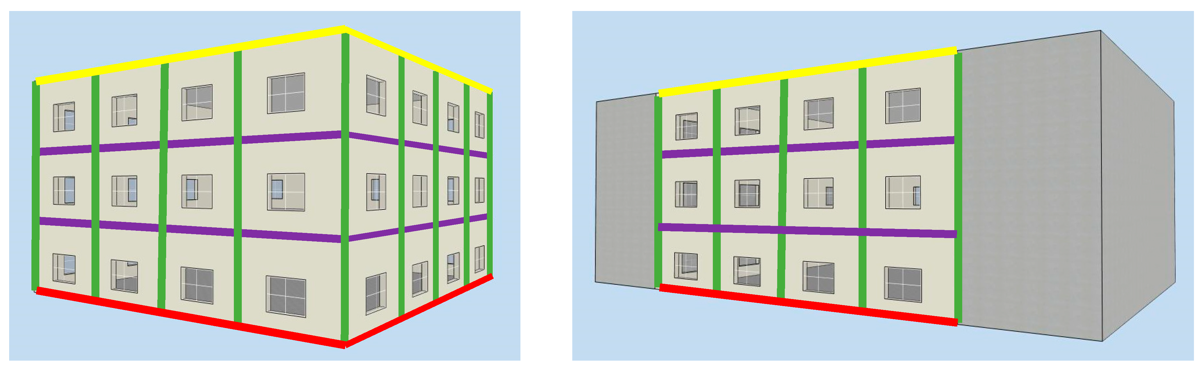
3.1. Results for the Detached House

A detached house means that a house is free of any shared walls and stands alone, i.e., all sides are exterior walls and interact with the outside conditions, as shown in Figure 1.

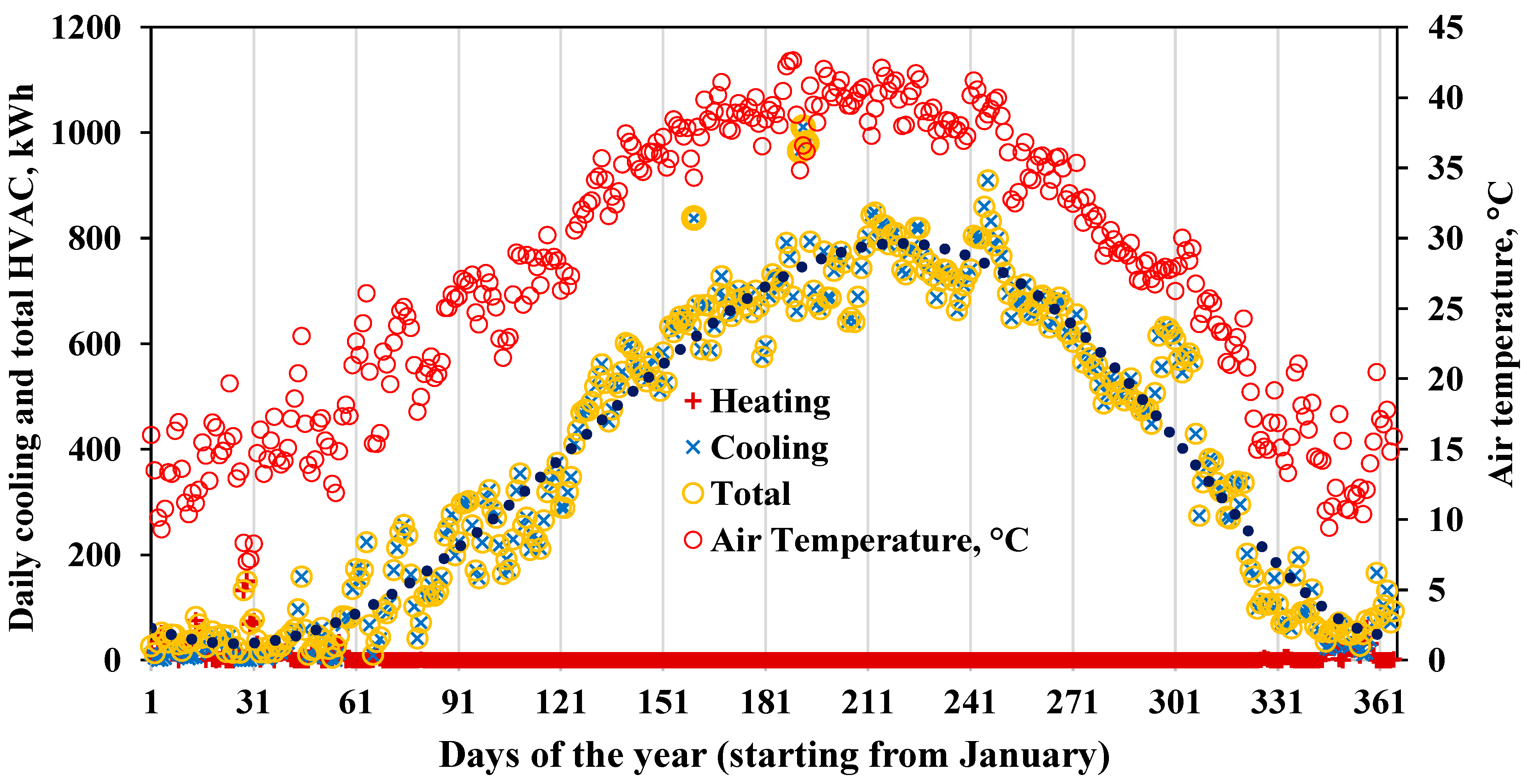
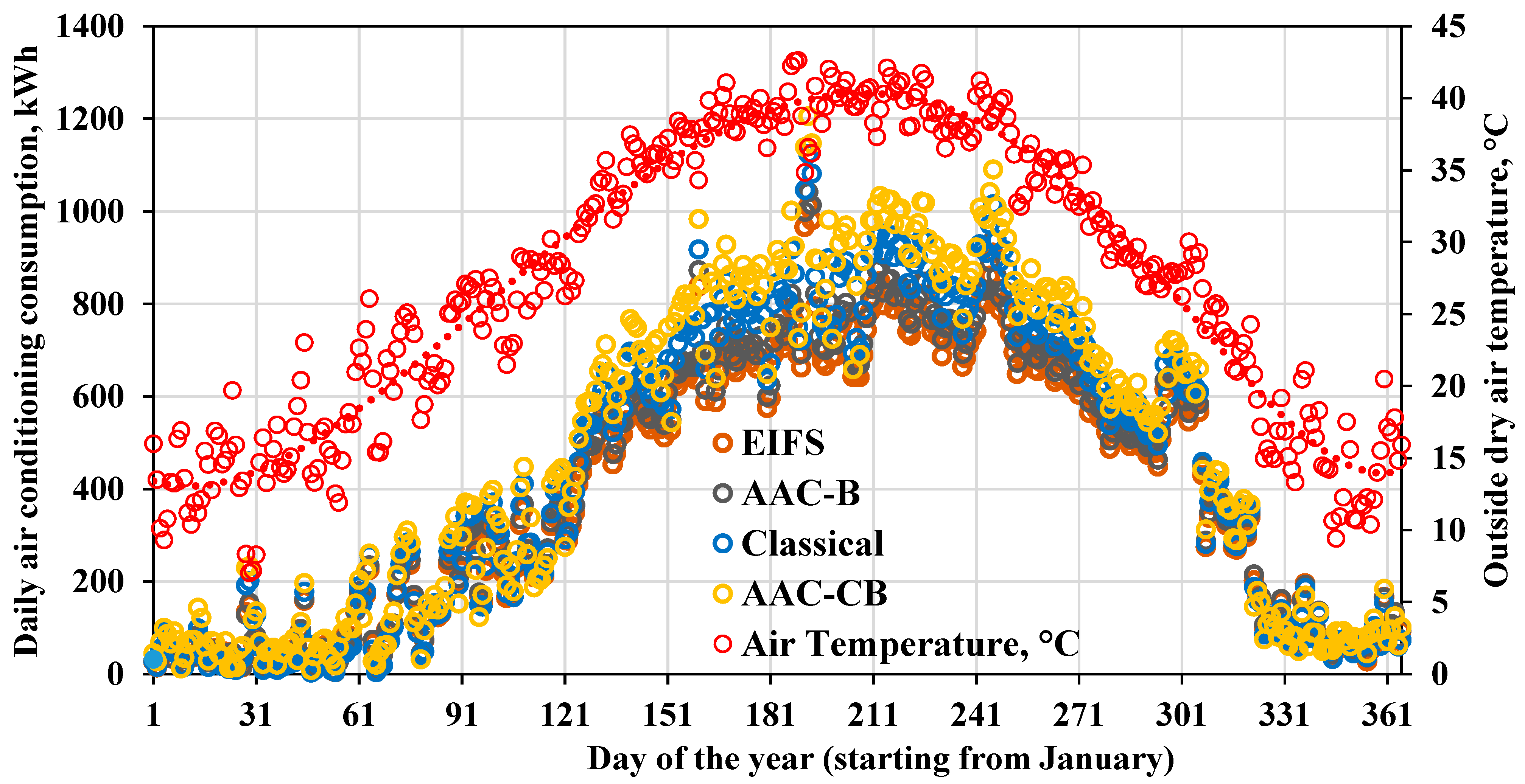
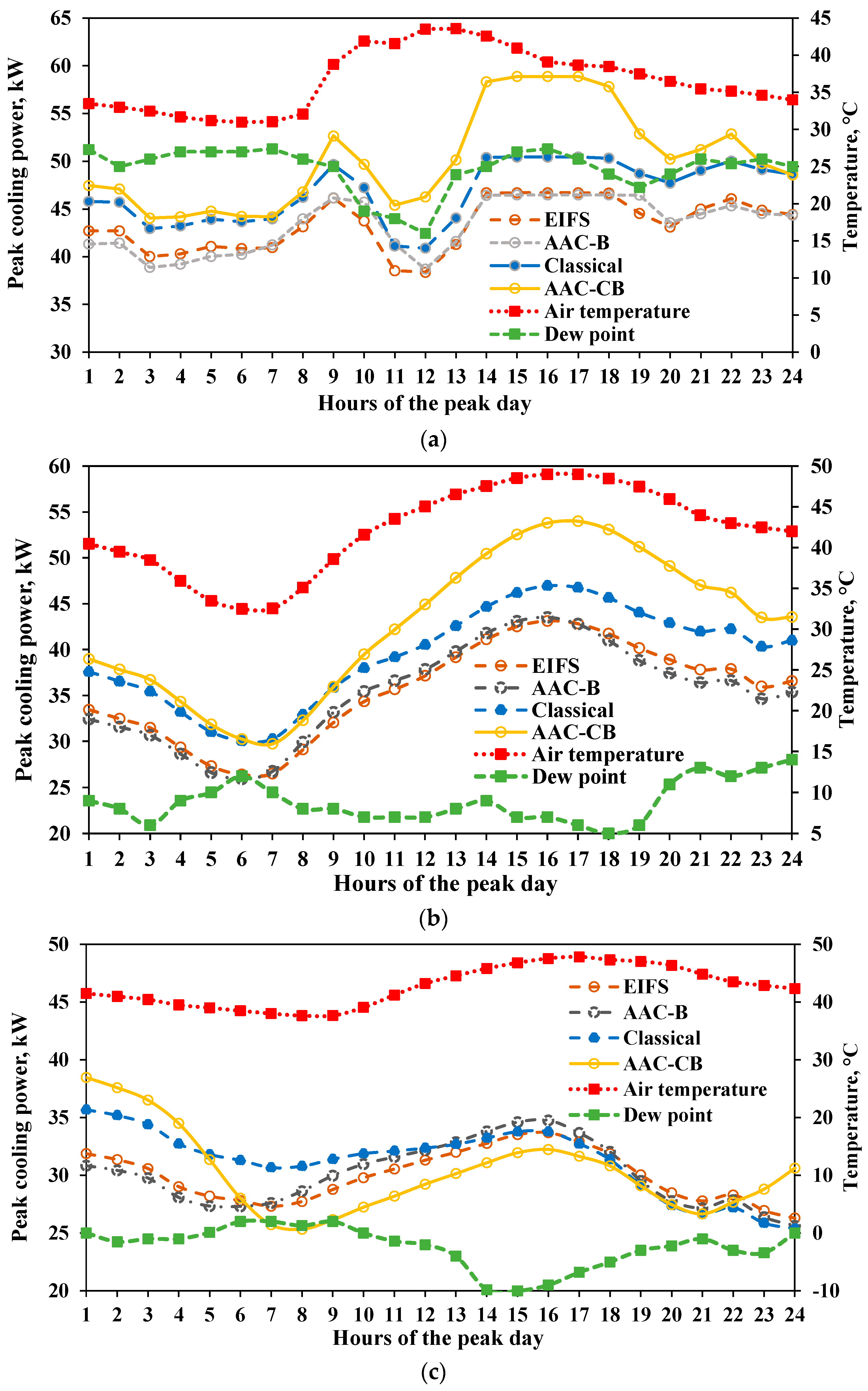
3.1.1. Daily Air Conditioning SYSTEM Consumption

Figure 4 shows the daily heating, cooling, and total (heating and cooling) electricity for the house constructed from the EIFS envelope throughout the year; moreover, the daily average ambient temperature is shown in Figure 4, where it varies from about 7.0 °C (29 January) to 42.6 °C (3 August). The maximum heating consumption is about 149.62 kWh (29 January) and the maximum cooling consumption is about 1010.45 kWh (11 July). The annual heating electricity is about 1.60 MWh whereas the annual cooling electricity is about 143.34 MWh. Thus, the annual heating electricity is very small (1.10%) compared to the cooling one (98.90%) in such a harsh hot climate. The heating load takes place during December, January, and February months; it is zero for the rest of the year when the cooling and total electricity becomes equal. In general, the pattern of the total load follows that of the outside air temperature. The scattered higher and lower points of the total daily electricity are the main symptoms of higher and lower humidity days. The highest load takes place on 11 July, while the highest ambient temperature occurs on 3 August. The average humidity ratio during the first day (11 July) is higher than the second day (3 August) by about 40%, while the ambient temperature of the first day is lower than the second by 5.51 °C.

Figure 5 shows the daily total electricity consumption of the air conditioning system for the studied detached house when the envelope is made from EIFS, AAC-B, classical, or AAC-CB wall types. In general, the lowest and largest consumption of the air conditioning system occurs for EIFS and AAC-CB house envelopes, respectively. The classical house envelope attains relatively lower consumption of the air conditioning system during some winter months (December, January, and February) that need a small heating load; this is because the thermal insulation is closer to the inner wall than the other envelopes, which is beneficial during the winter months. On annual bases, the average daily consumption for the EIFS, AAC-B, classical, and AAC-CB envelopes is 397.1, 411.9, 442.9, and 479.3 kWh, respectively, whereas their maximum daily consumptions are 1010.5, 1041.4, 1123.8, and 1205.3 kWh. The house envelopes made from AAC-B, Classical, and AAC-CB require larger average consumption than the EIFS envelope by 3.1, 11.2, and 19.3%, respectively.

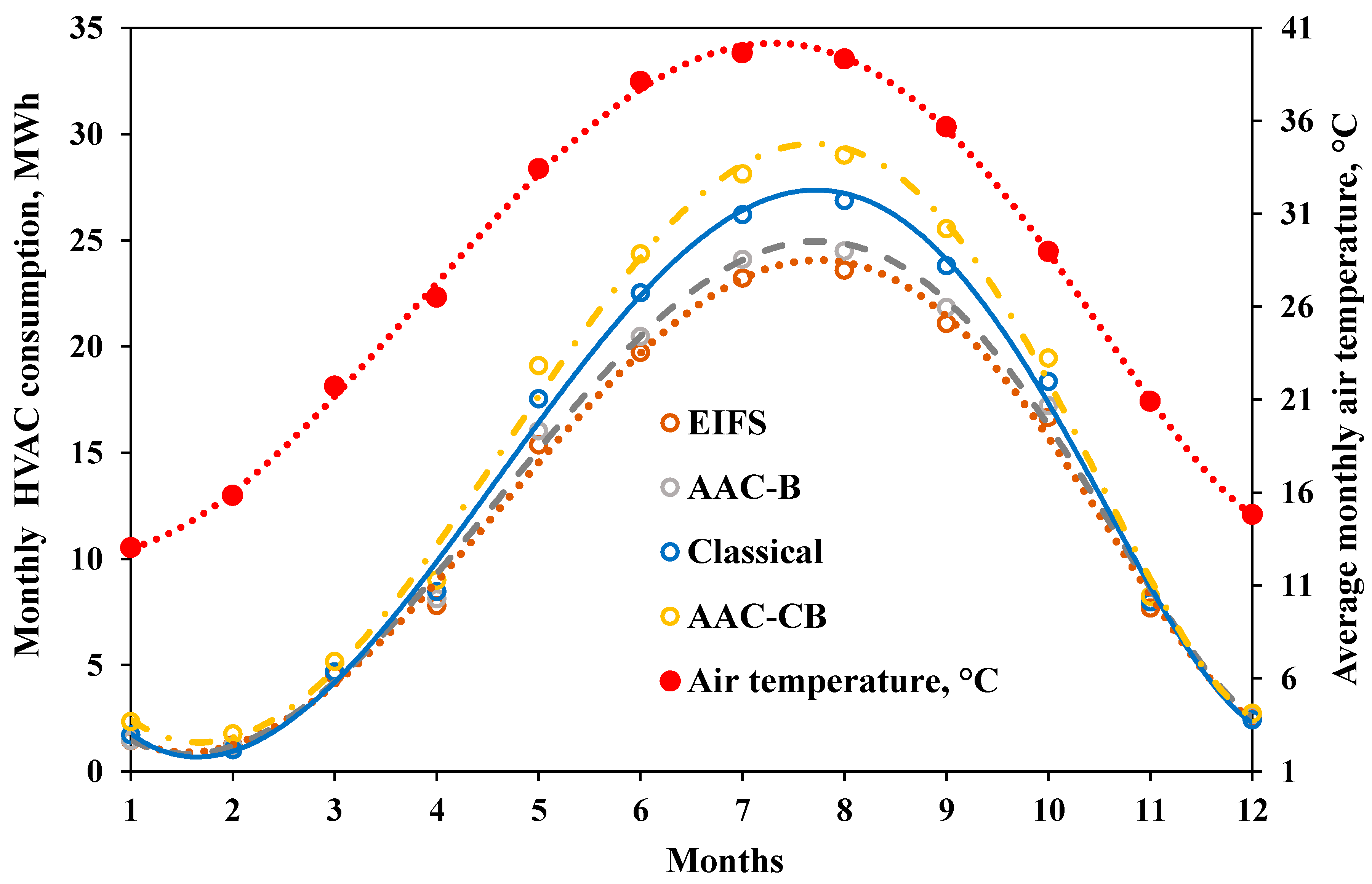
3.1.2. Monthly and Annual Air Conditioning System Consumption

Figure 6 shows the average monthly air temperature and the total energy consumption of the air conditioning system for the considered house with envelopes of EIFS, AAC-B, classical, and AAC-CB. Generally, the trend of air conditioning system energy follows the trend of the average outdoor air temperature with the maximum consumption taking place during the summer months of July and August. Again, the house envelopes made from EIFS, and AAC-B require lower and comparable consumption of the air conditioning system than those made from classical and AAC-CB with the latter having the maximum consumption. The maximum monthly consumption of the air conditioning system in August is about 23.60, 24.50, 26.88, and 29.02 MWh for the detached house with envelopes of EIFS, AAC-B, classical, and AAC-CB, respectively.

On the other hand, the annual energy consumption of the air conditioning system using EIFS, AAC-B, classical, and AAC-CB house envelopes is 144.94, 150.36, 161.66, and 174.94 MWh, respectively. The annual air conditioning system consumption for AAC-B, classical, and AAC-CB wall types is larger than that of EIFS by about 3.74, 11.53, and 20.70%, respectively.

3.1.3. Air Conditioning System Capacity

The capacity of the air conditioning system should be capable to handle the maximum hourly load of the considered house. Three days are carefully chosen to evaluate the hourly peak loads of the studied houses, under severe conditions, while using the four wall types. Figure 7a,b shows the hourly dry bulb temperature and relative humidity of the three selected days. The most humid day of the year is 11 July, where the relative humidity varies from 20.0 to 80.8% with an average value of 54.26%, whereas the average temperature is 36.60 (31.0–43.6) °C. Two hot days with average temperatures of 42.63 (37.3–48.0) °C and 42.11 (32.5–49.0) °C are chosen. The average relative humidity on the first day (8 July) is 6.58%, and on the second day (3 August) is 14.6%. Thus, July 8 presents the hottest-dry day, and August 3 presents a hot day with average relative humidity. Figure 7a shows that the maximum temperature takes place around 4–5 p.m. during hot days and around 12–1 p.m. during very humid days.

Figure 8 shows the power of the air conditioning system for the three selected days that represent the severe weather conditions: Figure 8a for the most humid day, Figure 8b for a hot day with mild humidity, and Figure 8c for the hottest and dry day. Figure 8a depicts the air conditioning system power on July 11 day, where the dew point varies from 16.0 to 27.3 °C (average 24.7 °C); this dew point indicates a very humid day where the humidity ratio reaches about 80.8% at 7 a.m. The power variation of the air conditioning system for all wall types follows the trend of the dew point temperature (green color), not the dry air temperature (red color). The maximum air conditioning system power takes place at about 3 p.m. for all wall types. On the other hand, Figure 8b shows the capacity of the air conditioning system during August 3 with an average dry air temperature of 42.11 °C and an average dew point of 8.3 °C (5.0 to 14.0 °C). In this case, the variations of the hourly air conditioner for all wall types follow the trend of the dry air temperature, not the dew point. The maximum cooling capacity for all wall types occurs at around 4 p.m. Note that the AAC-CB wall type showed very large variations of air conditioning system capacity compared with the other wall types. Figure 8c illustrates the air conditioning system capacity on a very dry hot day with an average dry air temperature of 42.6 °C (37.3 to 48.0 °C) and an average dew point of −2.4 °C (−10.0 to 2.0 °C).

The EIFS, AAC-B, and classical wall types showed more stable variations than the AAC-CB wall type, which proved to be less stable under very dry and hot air conditions; this signifies the effect of the static and dynamic characteristics of the house envelope type, including the house envelope heat capacity and the characteristics of the thermal bridges, on its expected air condition capacity. Table 1 indicates that the AAC-CB has lower heat capacity and thermal resistance than the other walls by 42.5–54.2% and 30.1–34.6%, respectively.

The required capacity of the air conditioner in the considered detached house using either of the four tested wall types is listed in

Table 5. The required air conditioning system capacity for the detached house under various weather conditions for the different wall types.

Day	Air Temp., °C	Dew Point, °C	Air Conditioning System Capacity, kW				Ratio of Air Conditioning System Capacity to That of EIFS
			EIFS	AAC-B	Classical	AAC-CB	EIFS	AAC-B	Classical	AAC-CB
11 July	36.6	24.7	46.71	46.48	50.45	58.88	1.00	1.00	1.08	1.26
3 August	42.1	8.3	43.12	43.50	46.95	53.99	1.00	1.01	1.09	1.25
8 July	42.6	−2.4	33.68	34.76	35.67	38.46	1.00	1.03	1.06	1.14
Average			41.17	41.58	44.36	50.44	1.00	1.01	1.08	1.23

; moreover, the ratio of the required air conditioning system capacity to that of EIFS is listed in Table 5. Clearly, house envelopes of EIFS and AAC-B require the lowest stable air conditioning system capacity under all weather conditions. AAC-CB needs the largest air conditioning system capacity, which is larger than that required by EIFS by about 23.0% on average. On the other hand, the average required air conditioning system capacity for the classical house envelope is larger than that required for the EIFS by about 8.0%.

Table 5 indicates that the largest required air conditioner capacity, for all house envelope types, takes place for the considerable latent load under the largest humid conditions (presented by the dew point), not the sensible load under high dry bulb temperature; this is attributed to the large latent heat needed to be extracted for the humid air compared to the sensible heat of the dry air, and is confirmed by the fact that the capacity required under warm and humid conditions is larger than in hottest and dry conditions by about 38.7% for EIFS, 33.7% for AAC-B, 41.4% for classical, and 53.1% for AAC-CB. These ratios confirm the sensitivity of the required air conditioning system power to the weather conditions for each wall type. The house envelope from AAC-CB is very sensitive (53.1%) whereas the other envelopes are less sensitive (33.7–41.4%) to the humid conditions of the outside air conditions. On the other hand, the air conditioning system capacity is sensitive to the house envelope type under the same weather conditions. The average capacity of the air conditioning system increases by 14 to 26% when the house envelope changes from EIFS to AAC-CB under the different tested weather conditions.

3.2. Results for the Attached House

In this work, an attached house means that the house shares three common wall sides of the property, i.e., it has only one façade in either of the main four directions (east, west, north, or south). Figure 1 illustrates the concept of the attached house considered in the present work.

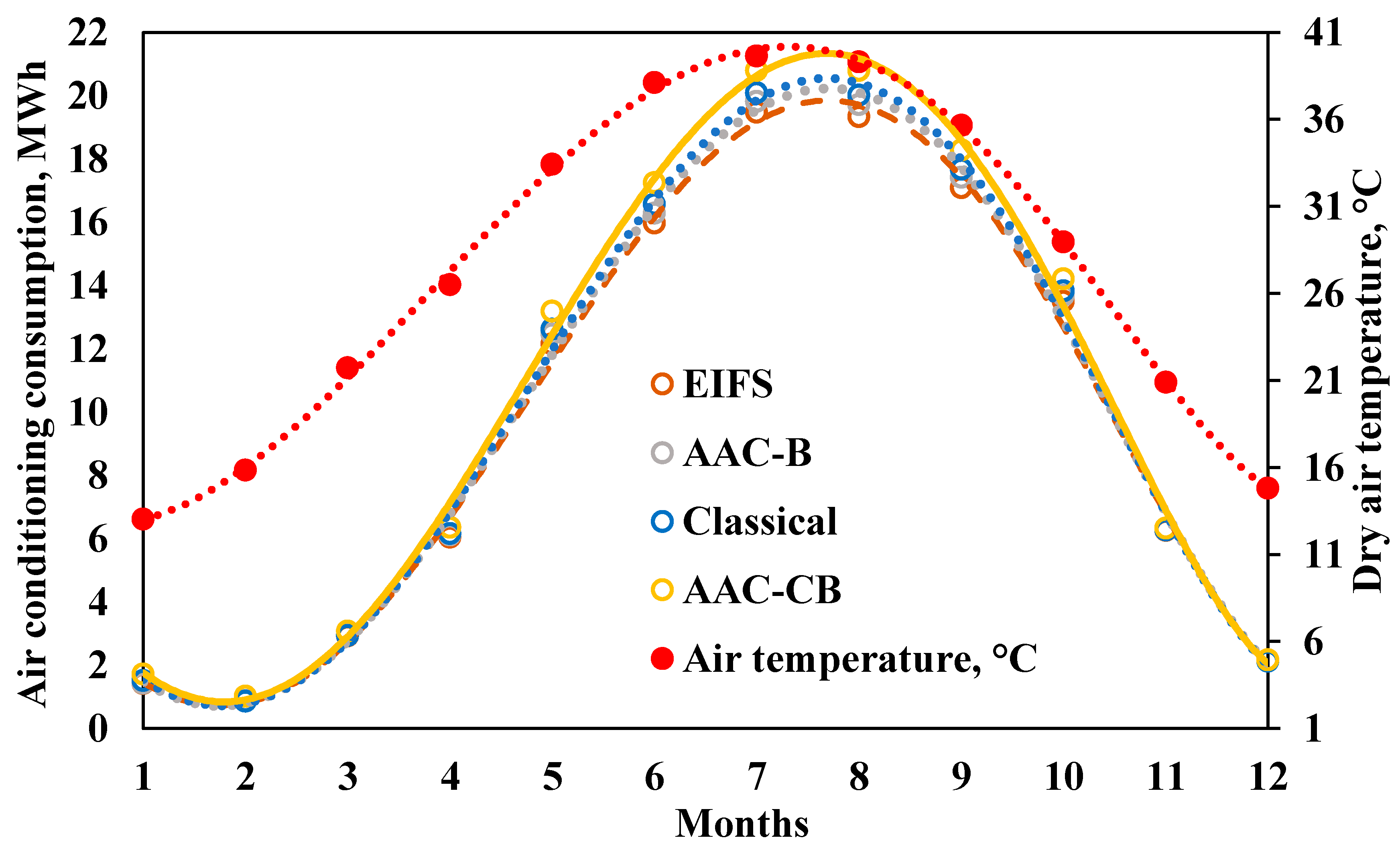
3.2.1. Air Conditioning System Consumption

As defined earlier, the attached house has only one façade in one of the main directions, whereas the other three wall sides are assumed adiabatic as they share their sides with the other attached houses. Figure 9 shows the difference in the daily consumption of the air conditioning system between either of the AAC-B, classical, and AAC-CB house envelopes and the EIFS house envelope for the considered three floors attached-house on the west façade (as a sample of the results of the other facades). The house with the west façade requires relatively larger consumption, of the air conditioning system, than the other facades on daily, monthly, and annual levels. In Figure 9, the positive values indicate lower consumption of the EIFS, and the negative values indicate larger consumption of the EIFS house envelope. It should be noted that the positive values reach up to 18.96, 27.07, and 56.4 kWh, whereas the negative values are limited to −12.13, −9.34, and −16.59 kWh for AAC-B, classical, and AAC-CB, respectively.

Figure 9 confirms that the EIFS house envelope performs better during the summer months (from 1 May to 18 November), whereas the consumption of the air conditioning system of the classical and AAC−CB house envelopes is relatively better during winter and mild months from December to April. The consumption difference of the air conditioning system used for houses with envelopes of EIFS and AAC−B is the lowest among the tested envelopes. Scattered data from one day to another reflects the variations in the outdoor dry bulb temperature and humidity ratio.

Figure 10 shows the monthly air conditioning system consumption of the considered attached house with the west façade (as a sample of the results of various facades) using the tested four envelopes. In general, the EIFS achieves the lowest, and the AAC−CB attains the largest air conditioning system consumption, particularly during the summer months. On the other hand, both AAC−CB and classical envelopes attain comparable consumption of the air conditioning system, for the west façade. Similar trends in the results are noticed for the other façades with the various tested envelopes. It should be noted that the difference in the air conditioning system consumption between envelopes of the detached house with the west façade is relatively smaller than that difference of the detached house (Figure 6); this is attributed to the considerable area exposed to the outside conditions of the detached house.

The annual air conditioning system consumption for the considered attached house using either of the four tested house envelopes when the house façade is in the east, west, north, or south direction is shown in Figure 11. As illustrated, the EIFS house envelope attains the lowest energy consumption for all facades. Obviously, the lowest air conditioning system consumption, for all house envelopes, takes place when the house has a north façade. The difference between the air conditioning system consumption on the west façade and that on the north façade is 4.40% for EIFS, 4.17% for AAC-B, 4.51% for classical, and 4.66% for AAC-CB house envelopes; this indicates that the orientation has a moderate effect on the envelope performance of the attached houses due to the relatively small area of the exterior wall (facade).

On the other hand, the largest consumption of the air conditioning system takes place for houses with the west façade, which is comparable to the east façade, for all house envelopes. Considering the consumption of the air conditioner using EIFS as a reference, the difference between the energy consumption using the various envelopes and that of the EIFS envelope is about 1.8 for AAC−B, 2.9% for classical, and 6.7% for AAC−CB. Thus, the effect of the house envelope type on the energy consumption of the air conditioning system of the considered attached house, in all orientations, is mild as it ranges between 1.8 and 6.7%.

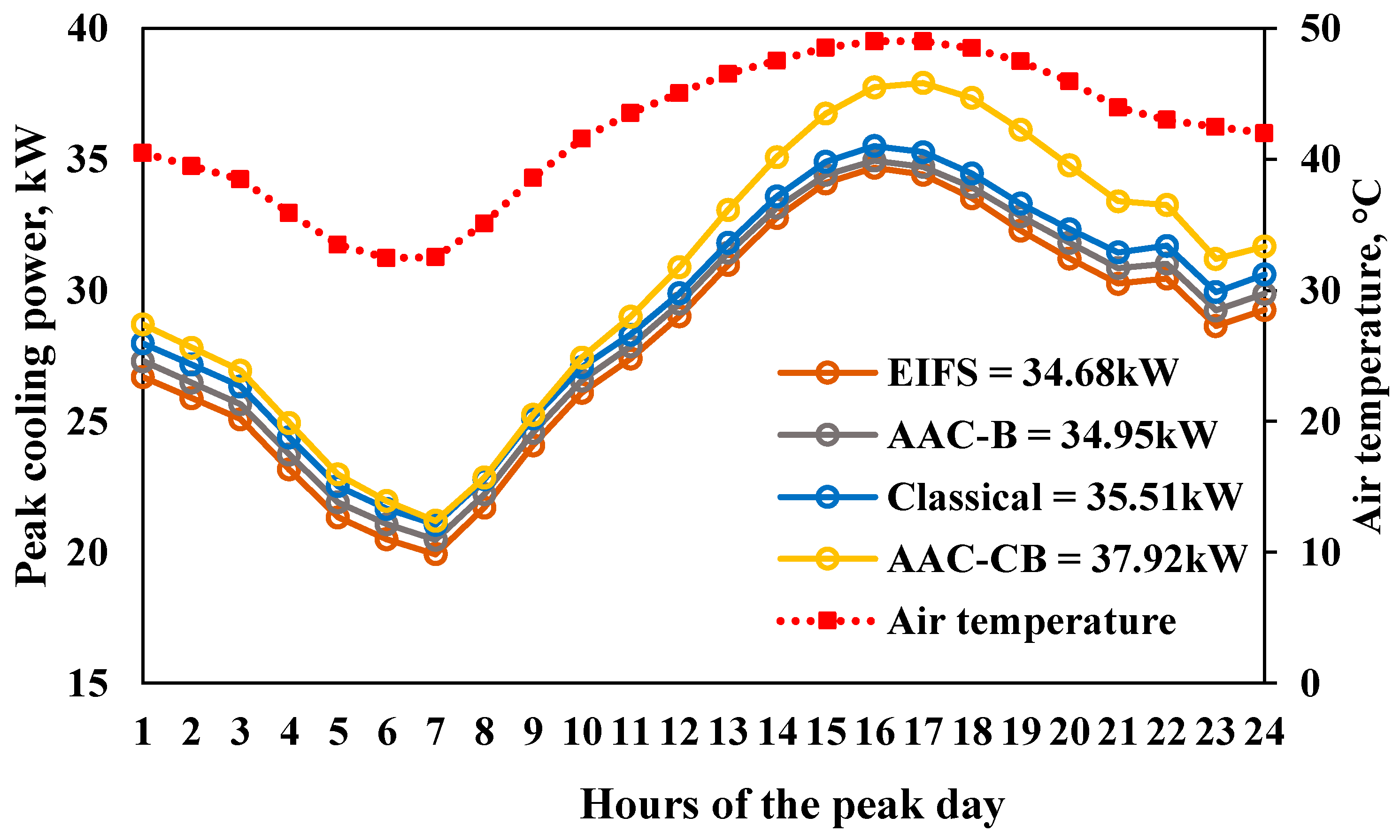
3.2.2. Air Conditioning System Capacity

Figure 12 shows the hourly air conditioning system capacity required for the representative peak day of 3 August (dry bulb temperature is 42.1 °C and the dew point is 8.3 °C) for the west façade as a sample. The power required by all house envelopes increases from 7 a.m. to 4 p.m. (or 5 p.m. for the AAC−CB envelope) when it reaches peak power and decreases for the rest of the day; this is a manifestation of the combined effect of the outdoor conditions (the solar radiation, dry air temperature, and dew point) and the building characteristics (the façade orientation, heat capacity, thermal diffusivity, thermal resistance, and radiation properties of the building components and thermal bridges). Accordingly, the power required for the air conditioning system should be taken as the maximum hourly power at 4 or 5 p.m. Continuously, the EIFS envelope required the lowest capacity followed by the AAC−B and classical whereas the AAC−CB envelope attains the largest air conditioning system capacity.

Figure 13 shows the required powers of air conditioning systems for the attached house on all façade orientations using the four building structures. The maximum peak power for all envelopes is required for the house with the west façade, followed by the east, south, and north facades; this order indicates the effect of the amount of solar radiation received on each façade. For all facades, the EIFS house envelope requires the lowest power of the air conditioning system followed by the AAC−B, classical, and AAC−CB house envelopes. The effect of the house envelope characteristics such as the heat capacity, thermal diffusivity, and thermal resistance of the envelope and thermal bridges control the stated order of the house envelope types in each direction. For example, the heat capacity of the EIFS wall is 1.74 times that of AAC wall, and 0.80 times that of the classical wall (Table 1). On the other hand, the total thermal resistance of the AAC−CB wall is lower than the other walls by 30.1 to 34.6%.

Figure 13 shows that the air conditioning system power required, in the west façade, ranges from 34.68 kW (EIFS) to 37.92 kW (AAC−CB) with a variation of about 9.34%. For the east façade, the air conditioning system power ranges from 33.75 to 36.61 kW with a variation of about 8.47%. The power variation of the air conditioning system between the various envelopes is about 9.12% (32.99–36.00 kW) in the south façade and 8.41% (32.82–35.58 kW) in the north façade. Thus, the average effect of the attached house envelope is about 8.84% for the main facades, with a standard deviation of 0.466.

3.3. Comparison between Detached and Attached Houses

The comparison between the detached and attached houses is based on two issues that are the annual air conditioning system consumption and the required air conditioning system capacity.

Table 6. Comparison of the annual air conditioning system consumption (MWh) between detached and attached houses for the different envelopes.

Façade	Annual Air Conditioning System Consumption (MWh)				Ratio of Detached to Attached Consumption
	EIFS	AAC−B	Classical	AAC−CB	EIFS	AAC−B	Classical	AAC−CB
West	117.21	119.25	120.68	125.23	1.237	1.261	1.340	1.397
East	117.05	119.13	120.54	125.00	1.238	1.262	1.341	1.400
South	116.21	118.28	119.54	124.10	1.247	1.271	1.352	1.410
North	112.27	114.48	115.47	119.65	1.291	1.313	1.400	1.462
Average	115.69	117.78	119.06	123.50	1.253	1.277	1.358	1.417
Detached	144.94	150.36	161.66	174.94	1.00	1.00	1.00	1.00
Average reduction	29.25	32.58	42.60	51.44

lists the annual consumption of the detached house and the attached house with the different considered façades using the four envelopes; moreover, listed the ratio of the annual consumption of the detached to that of the attached houses. On average, the annual air conditioning system consumption of the detached house is larger than that of the attached house by about 29.25, 32.58, 42.60, and 51.44 MWh for the EIFS, AAC-B, classical, and AAC-CB walls, respectively. Thus, the annual consumption of the detached house is larger than the average consumption of the attached house by about 25.3, 27.7, 35.8, and 41.7% for the EIFS, AAC−B, classical, and AAC−CB walls, respectively.

Table 7. The required air conditioning system capacity for the attached house under the peak weather conditions (dry bulb temperature is 42.1 °C and the dew point is 8.3 °C) for the different envelopes.

Façade	Air Conditioning System Capacity (kW)				Ratio of Detached to Attached AC Capacity
	EIFS	AAC−B	Classical	AAC−CB	EIFS	AAC−B	Classical	AAC−CB
West	34.68	34.95	35.51	37.92	1.243	1.245	1.322	1.424
East	33.75	34.30	34.70	36.61	1.278	1.268	1.353	1.475
South	32.99	33.50	33.83	36.00	1.307	1.299	1.388	1.500
North	32.82	33.35	33.66	35.58	1.314	1.304	1.395	1.517
Average	33.56	34.03	34.43	36.53	1.285	1.278	1.364	1.478
Detached	43.12	43.50	46.95	53.99	1.00	1.00	1.00	1.00
Average reduction	9.56	9.48	12.53	17.46

lists the required capacity of the air conditioning system for the attached house using the four different envelopes in either of the four main facades; moreover, listed the required air conditioning system capacity for the detached house and the ratio of air conditioning system consumption of the detached to that of the attached houses. On average, the required power of the detached house is larger than that of the attached house by about 9.56, 9.48, 12.53, and 17.46 kW, which is equivalent to 28.5, 27.8, 36.4, and 47.8% for EIFS, AAC-B, classical, and AAC-CB house structures.

4. Concluding Discussion

The effect of wall type on the detached house is higher than on the attached house; this is mainly due to the larger exposed area to the environment of the detached houses. Large-exposed area to the atmosphere yields more heat exchange and a substantial effect of thermal bridges and vice versa. Thus, the heat exchange with the environment through the envelope elements and the thermal bridge of the detached house is higher. Accordingly, a proper selection of the wall type of the detached houses is more crucial than the attached houses. However, the difference in the heat exchange between the attached and detached houses may be explained as follows: Unlike the detached house, the indoor temperature across both sides of the attached walls is similar. Thus, the attached wall is guessed to be adiabatic, and the heat exchange through the attached walls and thermal bridges is negligible compared to the detached walls that are exposed to the environment. Thus, the heat exchange depends on the wall area exposed to the environment for either an attached or detached house.

The effect of thermal bridges on the house thermal performance may be minimized by adding an uninterrupted (continuous) layer of insulation to the house envelope; this layer minimizes the bypassed heat leakage through thermal bridge areas. The uninterrupted layer of insulation can be practically applied to the external layer of the wall to avoid slabs on the roof and ground of each floor. Then, the insulation layer is covered by another durable cladding layer to protect the insulation from environmental impacts.

The comparison between the different tested wall types indicated that although the EIFS wall has a thermal resistance lower than the AAC−B and classical walls (Table 1), its thermal performance is much better than the other walls because of the uninterrupted external insulation layer. The main difference between the EIFS and the classical walls is the location of the thermal insulation. While the EIFS has continuous insulation in the external layer, the classical wall has the insulation between the two cement blocks; this insulation layer is interrupted by the concrete slabs of the roof and the ground of each floor. On the other hand, the AAC−B has a smaller area of thermal bridges than the other tested walls due to the absence of columns in the buildings made of this wall type; however, the use of this type of wall is limited to low-rise buildings only.

5. Conclusions

The effect of house wall type on the daily, monthly, and annual consumption of the air conditioning system of detached and attached houses (three floors each is 20 × 20 × 4 m³) in a hot climate is investigated. The tested four envelope types are exterior insulation and finish system (EIFS), autoclaved aerated concrete block (AAC−B), classical (cement blocks with insulation in between), and AAC column and beam (AAC−CB). The capacity of the air conditioning system of the detached house is determined based on the peak power of three selected days with extreme weather conditions such as very hot−dry, warm−very humid, and very hot−average humid days; moreover, the air conditioner power of the attached house with east, west, north, or south façade is evaluated on a very hot-average humid day. The consumption of the attached and detached houses is compared, under the same weather conditions. Based on the reported results, the following conclusions may be drawn:

• The average daily consumptions for the detached house with envelopes of EIFS, AAC−B, classical, and AAC−CB envelopes are 397.1, 411.9, 442.9, and 479.3 kWh, respectively. The maximum monthly consumptions of the air conditioning systems occur in August are about 23.60, 24.50, 26.88, and 29.02 MWh for the detached house with envelopes of EIFS, AAC−B, classical, and AAC−CB, respectively.
• The annual energy consumption of the air conditioning systems using EIFS, AAC−B, classical, and AAC−CB house envelopes are 144.94, 150.36, 161.66, and 174.94 MWh, respectively. Thus, the annual consumption of the air conditioning systems for the detached house using AAC−B, classical, and AAC−CB envelopes are larger than that of EIFS by about 3.74, 11.53, and 20.70%, respectively.
• The air conditioner capacities, for the detached house envelope types, under warm and humid conditions are larger than under hottest and dry conditions by about 38.7% for EIFS, 33.7% for AAC−B, 41.4% for classical, and 53.1% for AAC−CB.
• The air conditioning system capacities are sensitive to the detached house envelope as it increases by 14 to 26% when the detached house envelope changes from EIFS to AAC−CB.
• The effect of the house envelope on the annual consumption of the air conditioning system of the detached house is larger than that of the attached house. For example, the EIFS envelope has lower consumption than other envelopes by 3.74–20.70% for the detached house, and 1.8–6.7% for the attached house.
• The air conditioner annual consumption of the detached house is larger than that of the attached house by about 25.3, 27.7, 35.8, and 41.7%; moreover, the air conditioner capacity of the detached house is larger than the average of the attached house by 28.5, 27.8, 36.4, and 47.8% for EIFS, AAC-B, classical, and AAC−CB house envelopes, respectively.
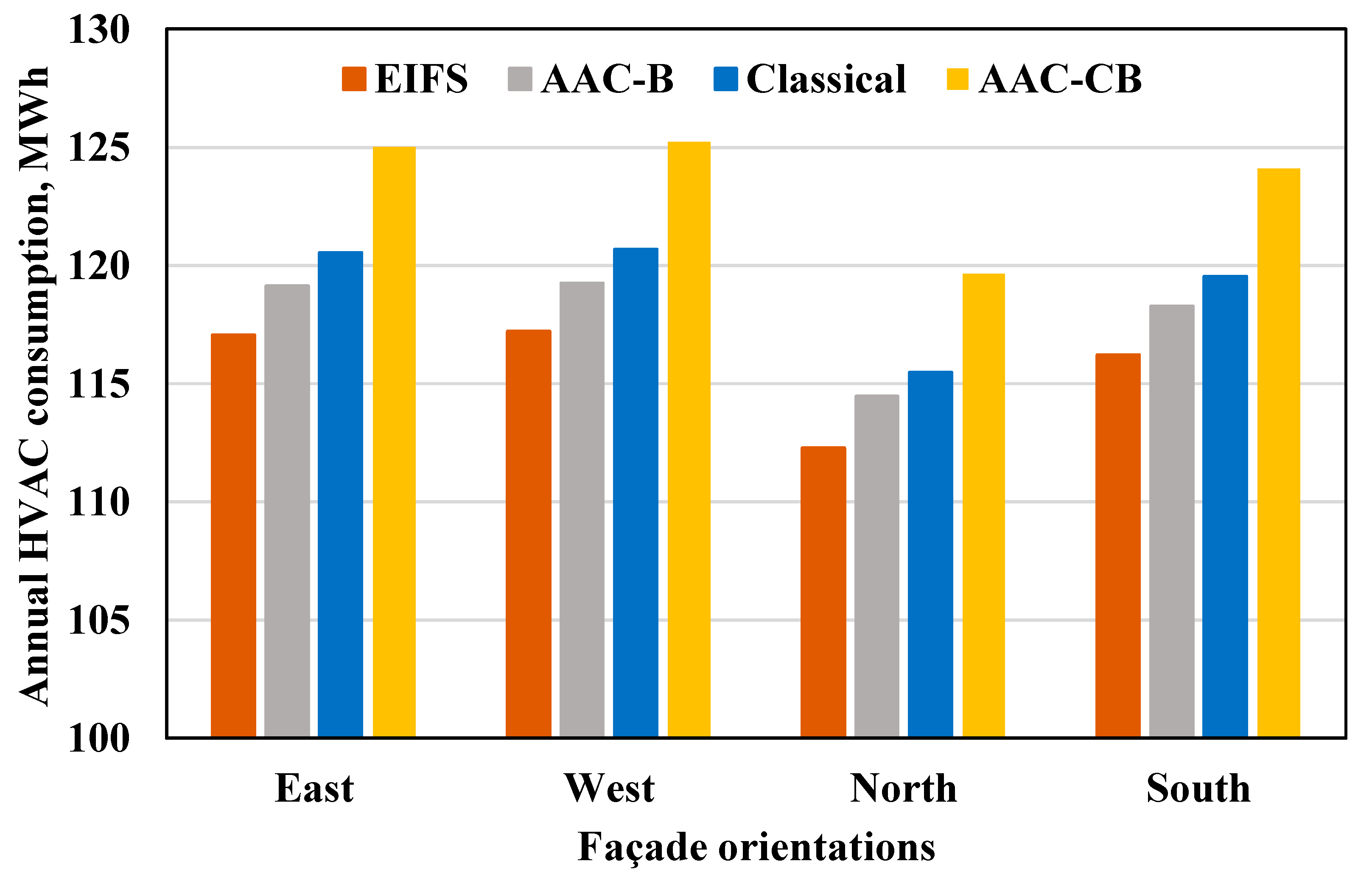
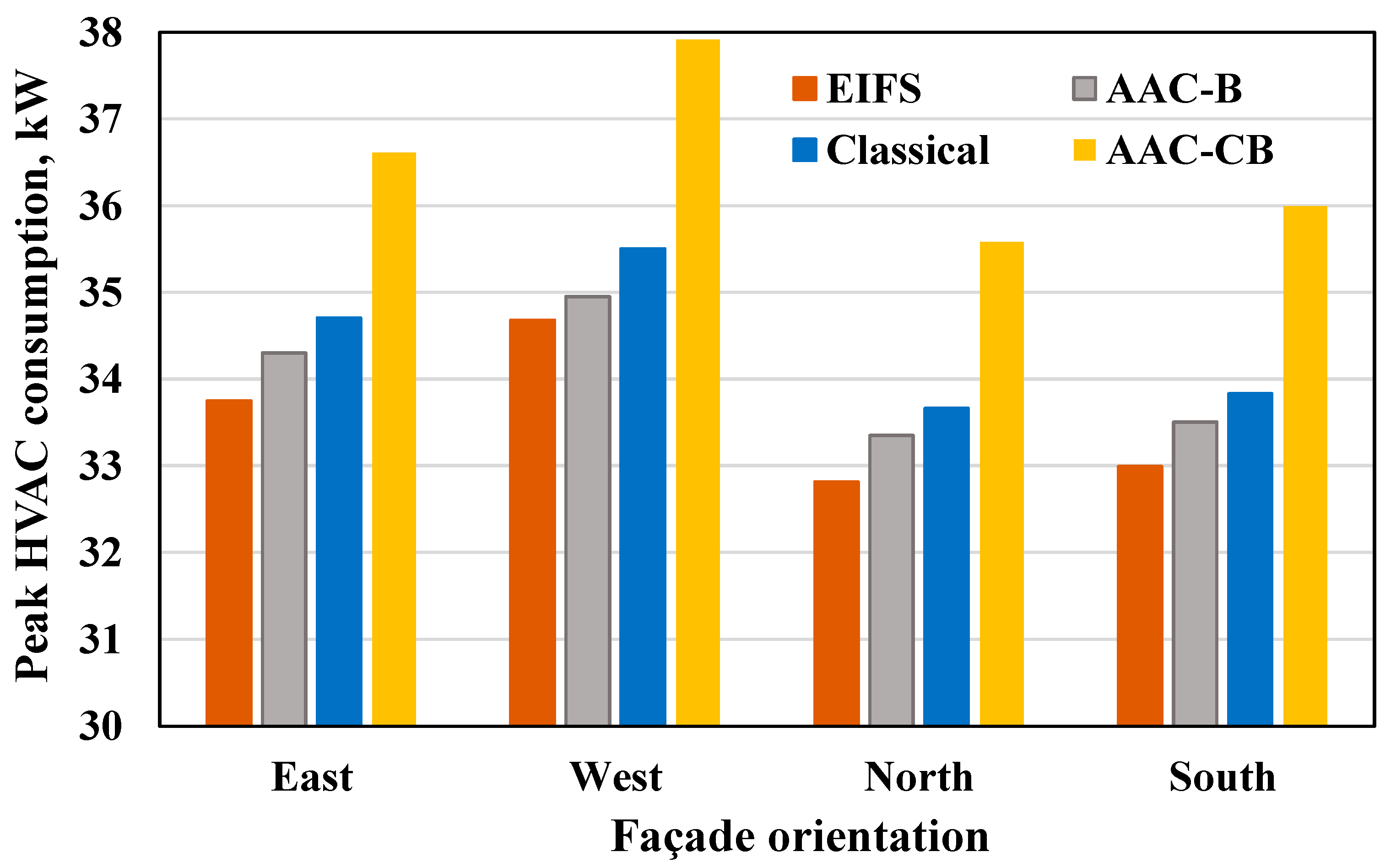
• The effect of the façade orientation on the envelope performance of the attached houses is moderate as the maximum difference between the annual consumption of the air conditioning system on the west and north façades is 4.40% and 4.66% for all houses envelopes.
• The average effect of the attached house envelope on the capacity of the air conditioning system is about 8.84%, with a standard deviation of 0.466%, for the different façade orientations (west, east, south, and north).

References

1. IEA. Key World Energy Statistics; Report for the Organization for Economic Cooperation and Development: Paris, France, 2014. [Google Scholar]
2. Ihm, P.; Krarti, M. “Design Optimization of Energy Efficient Residential Buildings in Tunisia”. Build. Environ. 2012, 58, 81–90. [Google Scholar] [CrossRef]
3. Menyhart, K.; Krarti, M. Potential energy savings from deployment of Dynamic Insulation Materials for US residential buildings. Build. Environ. 2017, 114, 203–218. [Google Scholar] [CrossRef]
4. Balaras, C.A.; Gaglia, A.G.; Georgopoulou, E.; Mirasgedis, S.; Sarafidis, Y.; Lalas, D.P. European residential buildings and empirical assessment of the Hellenic building stock, energy consumption, emissions and potential energy savings. Build. Environ. 2007, 42, 1298–1314. [Google Scholar] [CrossRef]
5. Waddicor, D.A.; Fuentes, E.; Sisó, L.; Salom, J.; Favre, B.; Jiménez, C.; Azar, M. Climate change and building ageing impact on building energy performance and mitigation measures application: A case study in Turin, northern Italy. Build. Environ. 2016, 102, 13–25. [Google Scholar] [CrossRef]
6. Harish, V.; Kumar, A. A review on modeling and simulation of building energy systems. Renew. Sustain. Energy Rev. 2016, 56, 1272–1292. [Google Scholar] [CrossRef]
7. Kosny, J.; Kossecka, E. Multi-dimensional heat transfer through complex building envelope assemblies in hourly energy simulation programs. Energy Build. 2002, 34, 445–454. [Google Scholar] [CrossRef]
8. ISO 14683; Thermal Bridges in Building Construction—Linear Thermal Transmittance—Simplified Methods and Default Values. International Organization for Standardization: Geneva, Switzerland, 2017.
9. DIN; Deutsches Institut für Normung e.V. Berlin. Beuth Verlag GmbH: Berlin, Germany, 2017.
10. Martin, K.; Erkoreka, A.; Flores, I.; Odriozola, M.; Sala, J.M. Problems in the calculation of thermal bridges in dynamic conditions. Energy Build. 2011, 43, 529–535. [Google Scholar] [CrossRef]
11. Viot, H.; Sempey, A.; Pauly, M.; Mora, L. Comparison of different methods for calculating thermal bridges: Application to wood-frame buildings. Build. Environ. 2015, 93, 339–348. [Google Scholar] [CrossRef]
12. Kossecka, E.; Kosny, J. Three-dimensional conduction z-transfer function coefficients determined from the response factors. Energy Build. 2005, 37, 301–310. [Google Scholar] [CrossRef]
13. Carpenter, S. Advances in Modelling Thermal Bridges in Building Envelopes. In Proceedings of the Canadian Conference on Building Energy Simulation, Ottawa, ON, Canada, 13–14 June 2001; Enermodal Engineering Limited: Kitchener, ON, Canada, 2001. [Google Scholar]
14. Kossecka, E.; Kosny, J. Equivalent wall as a dynamic model of complex thermal structure. J. Build. Phys. 1997, 40, 249–268. [Google Scholar] [CrossRef]
15. Aguilar, F. Transient modelling of high-inertial thermal bridges in buildings using the equivalent thermal wall method. Appl. Therm. Eng. 2014, 67, 370–377. [Google Scholar] [CrossRef]
16. Nagata, A. A Simple Method to Incorporate Thermal Bridge Effects into Dynamic Heat Load Calculation Programs. In Proceedings of the Ninth International IBPSA Conference, Montreal, PQ, Canada, 1 June 2005; pp. 817–822. [Google Scholar]
17. Xiaona, X.; Yi, J. Equivalent slabs approach to simulate the thermal performance of thermal bridges in building constructions. Proc. Build. Simul. 2007, 10, 287–293. [Google Scholar]
18. Xie, X.; Jiang, Y.; Xia, J. A new approach to compute heat transfer of ground-coupled envelope in building thermal simulation software. Energy Build. 2008, 40, 476–485. [Google Scholar] [CrossRef]
19. Martin, K.; Escudero, C.; Erkoreka, A.; Flores, I.; Sala, J.M. Equivalent wall method for dynamic characterization of thermal bridges. Energy Build. 2012, 55, 704–714. [Google Scholar] [CrossRef]
20. Quinten, J.; Feldheim, V. Dynamic modelling of multidimensional thermal bridges in building envelopes: Review of existing methods, application and new mixed method. Energy Build. 2016, 110, 284–293. [Google Scholar] [CrossRef]
21. Theodosiou, T.G.; Papadopoulos, A.M. The impact of thermal bridges on the energy demand of buildings with double brick wall constructions. Energy Build. 2008, 40, 2083–2089. [Google Scholar] [CrossRef]
22. Li, B.; Guo, L.; Li, Y.; Zhang, T.; Tan, Y. Thermal Bridge Effect of Aerated Concrete Block Wall in Cold Regions. IOP Conf. Ser. Earth Environ. Sci. 2018, 108, 022041. [Google Scholar] [CrossRef]
23. Al-Awadi, H.; Alajmi, A.; Abou-Ziyan, H. Effect of Thermal Bridges of Different ExternalWall Types on the Thermal Performance of Residential Building Envelope in a Hot Climate. Buildings 2022, 12, 312. [Google Scholar] [CrossRef]
24. Quinten, J.; Feldheim, V. Mixed equivalent wall method for dynamic modelling of thermal bridges: Application to 2-D details of building envelope. Energy Build. 2019, 183, 697–712. [Google Scholar] [CrossRef]
25. ISO 10211; Thermal Bridges in Building Construction—Heat Flows and Surface Temperatures—Detailed Calculations. International Organization for Standardization: Geneva. Switzerland, 2017.
26. Carlw Crawley, D.B.; Hand, J.W.; Kummert, M.; Griffith, B.T. Contrasting the capabilities of building energy performance simulation programs. Build. Environ. 2008, 43, 661–673. [Google Scholar] [CrossRef] [Green Version]
27. MEW. Energy Conservation Code for Buildings—Code of Practice (Mew/r-6/2018); Ministry of Electricity and Water: Safat, Kuwait, 2018.
28. Alajmi, A.F. Implementing the Integrated Design Process (IDP) to design, construct and monitor an eco-house in hot climate. Int. J. Sustain. Eng. 2021, 14, 630–646. [Google Scholar] [CrossRef]
Figure 1. Typical illustration of a detached house (left) and an attached house (right), with the locations of the thermal bridges on the roof (yellow), intermediate floor slab (purple), slab-on-grade (red), and concrete column (green).
Energies 15 04493 g001
Figure 2. Thermal bridges for EIFS. (a) the intermediate Floor slab, (b) roof, (c) slab on grade, and (d) column beam (colored continuous lines represent the isothermal temperature contours and arrows represent the heat flow directions).
Energies 15 04493 g002
Figure 3. Flow diagram of the determination of the dynamic wall properties using equivalent wall method.
Energies 15 04493 g003
Figure 4. Daily heating, cooling, and total HVAC consumption for the three floors detached house with building envelopes made from EIFS wall type.
Energies 15 04493 g004
Figure 5. Daily air conditioning consumption for the three floors detached house with building envelopes made from four different wall types.
Energies 15 04493 g005
Figure 6. Monthly air conditioning consumption for the three floors detached house with building envelopes made from four different wall types.
Energies 15 04493 g006
Figure 7. Weather conditions of the three selected days (Average values are shown between parenthesis). (a) Dry bulb temperature of the three selected days, (b) Relative humidity of the three selected days.
Energies 15 04493 g007
Figure 8. Hourly air conditioning consumption for the three floors detached house with building envelopes made from four different wall types during the peak days. (a) For a very humid day: air temperature = 36.6 °C, dew point = 24.7 °C (11 July), (b) For a hot and dry day: air temperature = 42.1 °C, dew point = 8.3 °C (3 August), and (c) For a hot and very dry day: air temperature = 42.6 °C, dew point = −2.4 °C (8 July).
Energies 15 04493 g008
Figure 9. Daily air conditioning consumption difference between each wall type and EIFS building envelope for the three floors attached house (west façade) with building envelopes made from four different wall types.
Energies 15 04493 g009
Figure 10. Monthly air conditioning consumption for the attached house (west facade) with building envelopes made from four different wall types.
Energies 15 04493 g010
Figure 11. Annual air conditioning consumption for the three floors attached house with different orientation facades for different building envelopes.
Energies 15 04493 g011
Figure 12. Hourly air conditioning consumption for the three floors attached house (west facade) with building envelopes made from four different wall types during the peak day (3 August).
Energies 15 04493 g012
Figure 13. Air conditioning capacity for the three floors attached house with different orientation facades for different building envelopes during the peak days.
Energies 15 04493 g013