
Statistical Analysis of Baseline Load Models for Residential Buildings in the Context of Winter Demand Response


Abstract
:1. Introduction
- Task 1: Are regression-type baseline load models significantly more accurate than other models?
- Task 2: For adjusted arithmetic baseline load models, do individual adjustments for each peak period provide additional overall precision to the baseline?
- Task 3: How do the performances of the baseline load models change with the number of events called during the DR season?
2. Materials and Methods
2.1. Data Sample and Processing
- Annual electricity consumption (>5000 kWh);
- Weather sensitivity (UA > 75 W/°C);
- Amount of missing data (<20%).
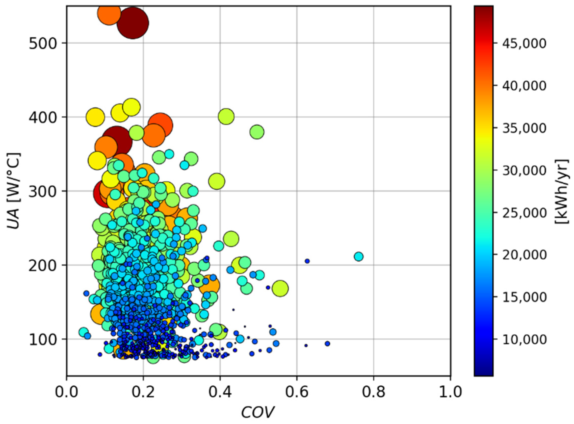
2.2. Sample Characterization
2.3. Proxy Event Days (PED)
2.4. Baseline Load Models
- Arithmetic (11 models); models using the hourly loads (Lh) of a certain number of admissible days (X) within a given baseline window (Y) to predict the baseline load ();Tested models include:
- High X of Y: with Y = 5 or 10 and X = 3, 4, 5 or 7, 8, 9, 10. These models consider only the X maximal Lh of the last Y admissible days [];
- Mid X of Y: with Y = 5 or 10 and X = 3, 6, or 8. These models discard the maximal and minimal Lh to keep only the X center ones;
- Monthly High 5: just like a High X of Y model with X = 5 and Y = duration of the billing period, in days (approximately a calendar month).
- Regression (2 models): Models using a correlation between the load and other variables (such as weather data, occupancy, weekday, production, etc.) to predict the load during a DR event. OAT is the only variable considered in this study as it is recognized to have the strongest effect on residential load profiles during winter in cold climate. The regression model is based on this equation:Tested models include:
- Seasonal weather: Historical data are used to calculate coefficients of a linear regression of hourly load to hourly OAT. The coefficients are calculated using data from all the heating season admissible days (1 December to 31 March).
- 10-day weather: Model using a similar linear regression as the seasonal weather model but the coefficients are calculated using data from only the ten previous admissible days.
- Matching-day: SGE model matches the conditions of the PED to the historic admissible day closest in terms of weather and operating conditions. Days with similar operating conditions are found using fuzzy c-mean clustering (unsupervised machine learning) of daily load consumption profile. Clustering of daily load profile is used to find days with similar operating conditions [35].
2.5. Baseline Adjustments
2.6. Performance Metrics
2.6.1. Bias Metric: MBE
2.6.2. Accuracy Metric: MAPE
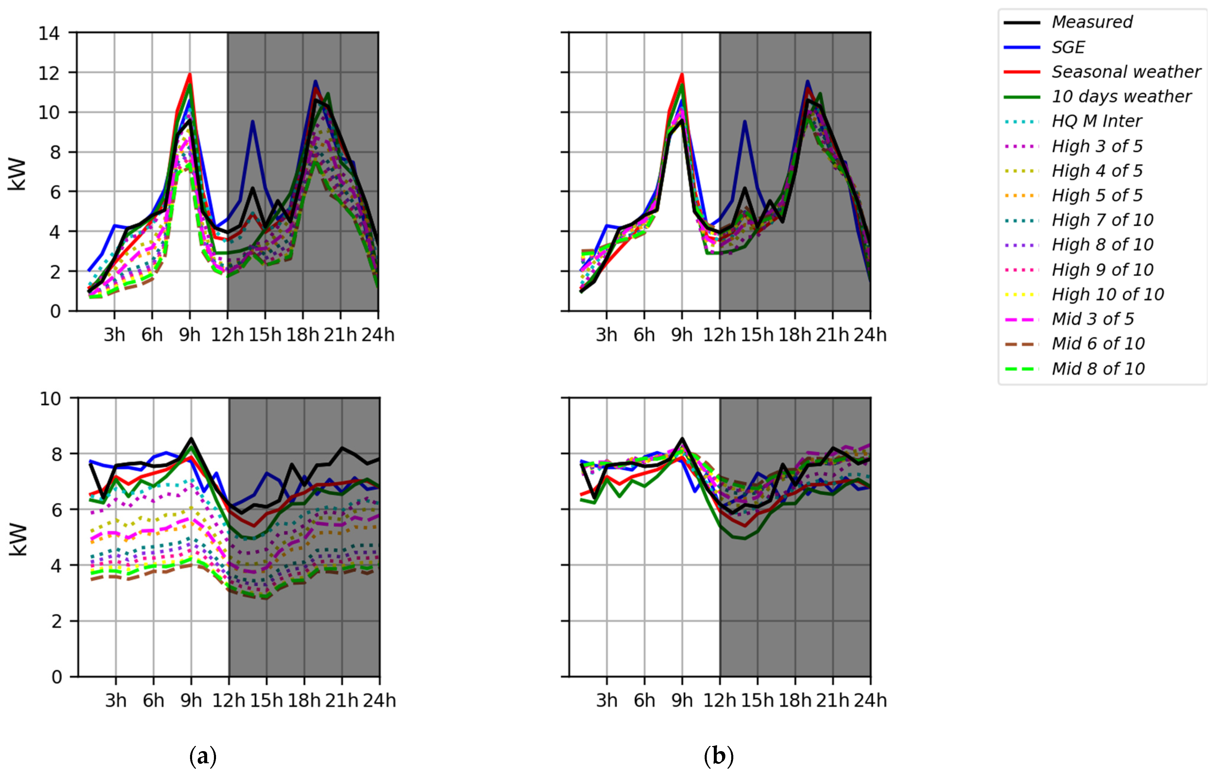
3. Results
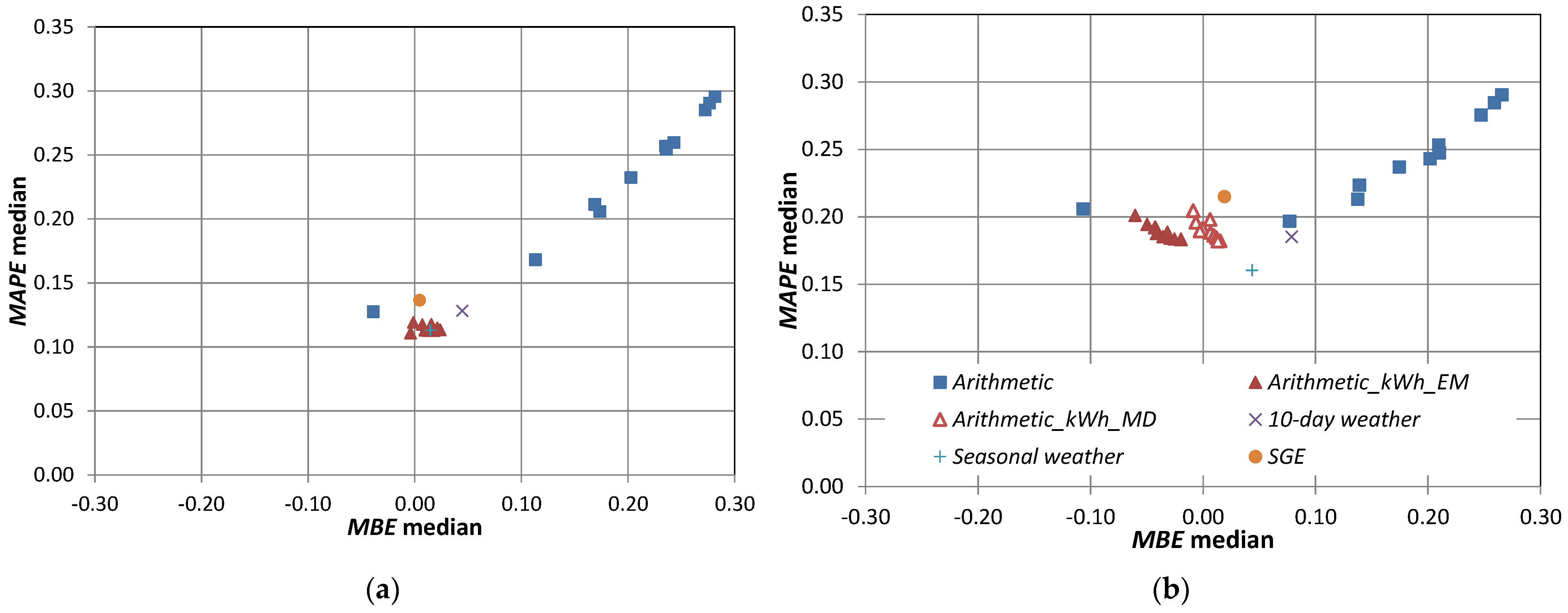
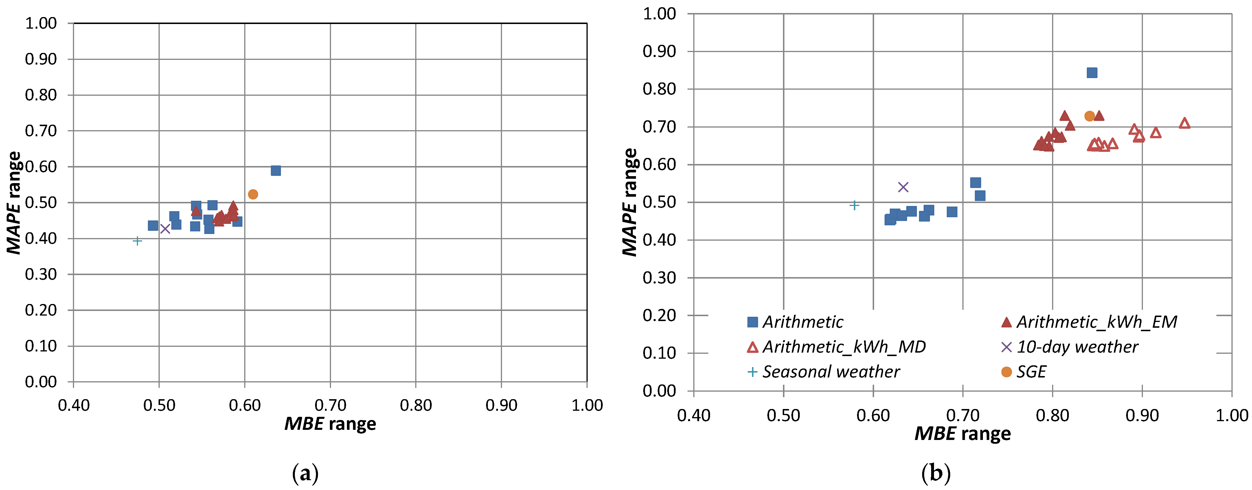
3.1. Models Ranking
- Arithmetic models have the largest median MBE combined with high MAPE values for both peak periods. Most of these models underestimate the load (median MBE > 0), except for Monthly High 5 which overestimates. Arithmetic models lead to some of the smallest range value for both metrics and peak periods;
- Compared to the Arithmetic models, Adjusted arithmetic models present a significant reduction in the distributions’ medians. Range value results show that baseline adjustments tend to widen the distributions, especially for the evening events. Performance’s metrics across Adjusted arithmetic models are similar, meaning none of the models really stand out;
- The SGE model presents slightly worse results than the best ones. The SGE model does not perform well, likely because it is based on load pattern recognition which is not compatible with the high-variability characteristics of residential load profiles;
- Apart from the Arithmetic models, the 10-day weather model has the biggest bias as shown by its MBE median values for both peak periods. However, its low range values indicate that it produced consistent results (narrow distributions);
- The Seasonal weather model is among the best performing models in terms of median and range value for both metrics and peak periods;
- For the morning period (Figure 4a and Figure 5a), the best Adjusted arithmetic models compare favorably with the Seasonal weather model especially in terms of bias. For the evening period, Seasonal weather has a slight advantage compared to the best Adjusted arithmetic models except for the MBE median, meaning that it is more biased.
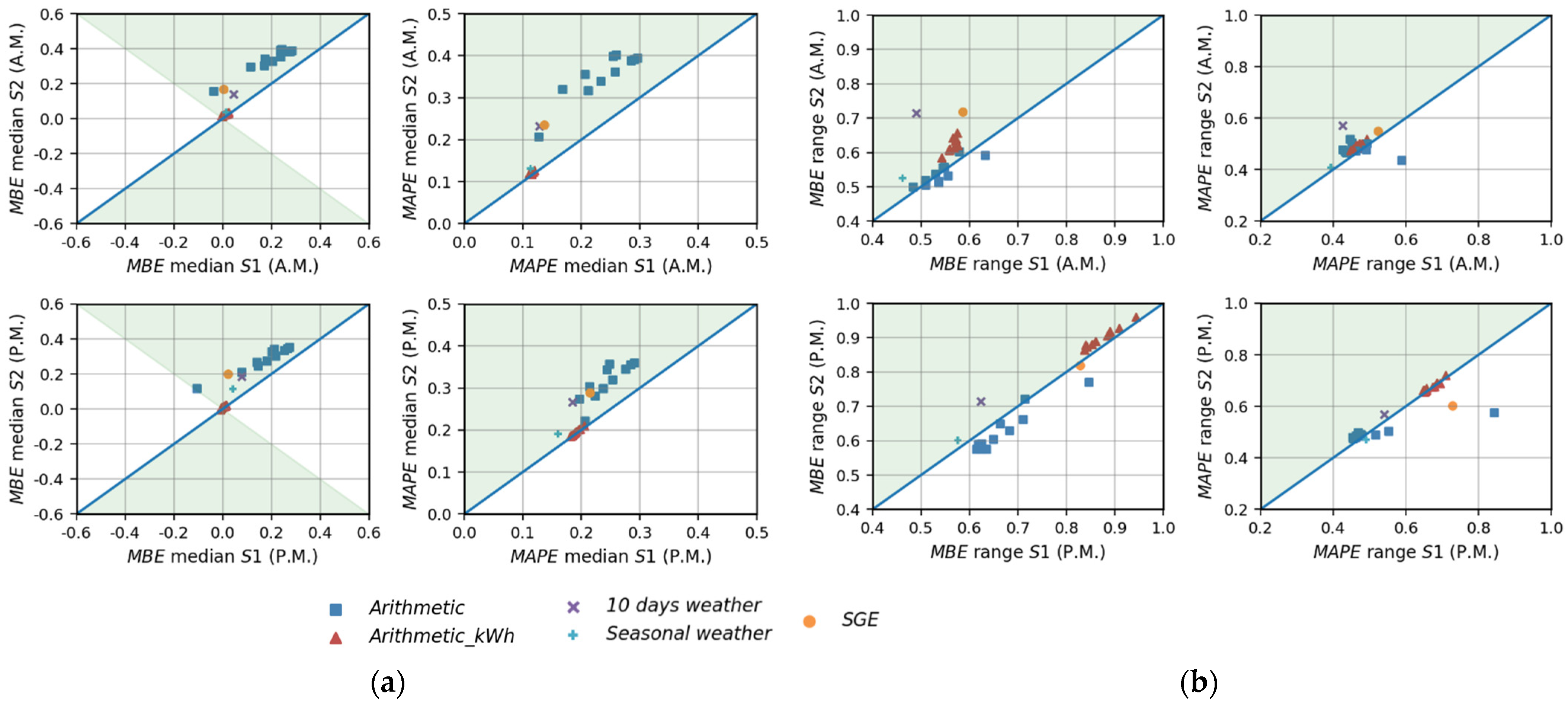
3.2. Effect of the Adjustment Window
3.3. Effect of the Number of Events on the Performance Metrics
4. Discussion
- Task 1: Are regression-based baseline load models significantly more accurate than other models?
- Task 2: For adjusted arithmetic models, do individual adjustments for each peak period provide additional precision to the baseline?
- Task 3: How does the repeated use of DR resources during the winter season affect the performances of the baseline load models?
5. Conclusions
Author Contributions
Funding
Institutional Review Board Statement
Informed Consent Statement
Data Availability Statement
Conflicts of Interest
References
- ANSI/ASHRAE/IES Standard 90.1-2016; American Society of Heating, Refrigerating and Air-Conditioning Engineers. Energy Standard for Buildings Except Low-Rise Residential Buildings. ASHRAE: Atlanta, GA, USA, 2016.
- Hydro-Québec. Comparaison des prix de L’électricité dans les Grandes Villes Nord-Américaines-Tarifs en Vigueur le 1er Avril 2021. 2021. Available online: https://www.hydroquebec.com/data/documents-donnees/pdf/comparaison-prix-electricite.pdf (accessed on 7 December 2021).
- Sabourin, M. Les programmes de vente devraient produire leurs effets en 1970. In Entre-nous; Hydro-Québec Archives: Quebec, QC, Canada, 1970; p. 8. [Google Scholar]
- Natural Resource Canada. Comprehensive Energy Use Database-Residential Sector-Quebec, Table 21. 2021. Available online: https://oee.nrcan.gc.ca/corporate/statistics/neud/dpa/showTable.cfm?type=CP§or=res&juris=qc&rn=21&page=0 (accessed on 7 December 2021).
- Hydro-Québec. Using Energy More Wisely in Cold Weather. 2021. Available online: https://www.hydroquebec.com/residential/customer-space/electricity-use/winter-electricity-consumption.html (accessed on 7 December 2021).
- Hydro-Québec. État D’Avancement 2021 du Plan D’Approvisionnement 2020–2029. 2021. Available online: http://www.regie-energie.qc.ca/audiences/Suivis/Suivi%20HQD_PlanAppro2020-2029/%C3%89tat%20d’avancement%202021.pdf (accessed on 7 December 2021).
- Fournier, M.; Leduc, M.; Sansregret, S.; Poulin, A. Making the Connection: Testing Line-Voltage Communicating Thermostats for Baseboard Heaters in DR and EE Experiments. In Proceedings of the 2018 ACEEE Summer Study on Energy Efficiency in Buildings, Pacific Grove, CA, USA, 12–17 August 2018. [Google Scholar]
- Federal Energy Regulatory Commission FERC. Reports on Demand Response and Advanced Metering. 2021. Available online: https://www.ferc.gov/industries-data/electric/power-sales-and-markets/demand-response/reports-demand-response-and (accessed on 7 December 2021).
- NV Energy. Cool Share Support. 2021. Available online: https://www.nvenergy.com/help/coolshare-support (accessed on 7 December 2021).
- PSEG Long Island. Smart Savers Thermostat Program. 2021. Available online: https://www.psegliny.com/saveenergyandmoney/energystarrebates/SmartSavers (accessed on 7 December 2021).
- American Society of Heating, Refrigerating and Air-Conditioning Engineers. ASHRAE Guideline 14-2014: Measurement of Energy, Demand and Water Savings; ASHRAE: Atlanta, GA, USA, 2014. [Google Scholar]
- IPMVP Committee. International Performance Measurement and Verification Protocol: Concepts and Options for Determining Energy and Water Savings; National Renewable Energy Lab.: Golden, CO, USA, 2001; Volume I, (No. DOE/GO-102001-1187; NREL/TP-810-29564). [Google Scholar]
- North American Energy Standards Board. WEQ-015 Measurement and Verification of Wholesale Electricity Demand Response, NAESB WEQ Business Practice Standards version 003.1; Standards and Models Relating to Measurement and Verification of Wholesale Electricity Demand Response, NAESB: Houston, TX, USA, 2015. [Google Scholar]
- CalTRACK. CalTRACK Technical Documentation: Modeling Hourly Methods. 2018. Available online: http://docs.caltrack.org/en/latest/index.html (accessed on 9 November 2021).
- Commonwealth Edison Company (ComEd). Peak Time Savings. 2021. Available online: www.comed.com/SmartEnergy/InnovationTechnology/Pages/PeakTimeSavingsFAQ.aspx#:~:text=ComEd%20will%20credit%20your%20energy,open%20and%20factories%20are%20running (accessed on 7 December 2021).
- PEPCO. About Peak Energy Savings Credit. 2021. Available online: www.pepco.com/WaysToSave/ForYourHome/Pages/MD/AboutPeakEnergySavingsCredit.aspx (accessed on 7 December 2021).
- Connexus Energy. Peak-Time Rebate. 2021. Available online: www.connexusenergy.com/save-money-and-energy/programs-rebates/peak-time-rebate (accessed on 7 December 2021).
- BGE. Energy Savings Days. 2021. Available online: www.bge.com/WaysToSave/ForYourHome/Pages/EnergySavingsDays.aspx (accessed on 7 December 2021).
- Portland General. Peak Time Rebates. 2021. Available online: https://portlandgeneral.com/ptr (accessed on 7 December 2021).
- Elliot, C.; Shelton, J.; Hanna, D. Challenges of estimating hourly baselines for residential customers. In Proceedings of the 2013 International Energy Program Evaluation Conference, Chicago, IL, USA, 13–15 August 2013. [Google Scholar]
- Goldberg, M.L.; Agnew, G.K. Measurement and Verification for Demand Response; US Department of Energy: Washington, DC, USA, 2013.
- Granderson, J.; Price, P.N. Development and application of a statistical methodology to evaluate the predictive accuracy of building energy baseline models. Energy 2014, 66, 981–990. [Google Scholar] [CrossRef] [Green Version]
- Goldberg, M.L.; Agnew, G.K. Protocol Development for Demand Response Calculation-Findings and Recommendations. 2003. Available online: www.calmac.org/publications/2002-08-02_XENERGY_REPORT.pdf (accessed on 17 June 2022).
- Bode, J.; Perry, M.; Morgan, S.; Freeman, S. Assessment of Settlement Baseline Methods for Ontario Power Authority’s Commercial & Industrial Event Based Demand Response Programs; Prepared by Freement, Sullivan & Co. for Ontario Power Authority: Toronto, ON, Canada, 2010. [Google Scholar]
- KEMA Inc. PJM Empirical Analysis of Demand Response Baseline Methods White Paper. PJM Load Management Task Force. 2011. Available online: www.pjm.com/-/media/markets-ops/demand-response/pjm-analysis-of-dr-baseline-methods-full-report.ashx (accessed on 17 June 2022).
- Granderson, J.; Sharma, M.; Crowe, E.; Jump, D.; Fernandes, S.; Touzani, S.; Johnson, D. Assessment of Model-Based peak electric consumption prediction for commercial buildings. Energy Build. 2021, 245, 111031. [Google Scholar] [CrossRef]
- EnerNoc. The Demand Response Baseline Whitepaper. 2009. Available online: www.naesb.org/pdf4/dsmee_group3_100809w3.pdf (accessed on 12 October 2021).
- George, S.; Bode, J.; Berghman, D. 2012 San Diego Gas & Electric Peak Time Rebate Baseline Evaluation. Prepared for San Diego Gas & Electric. 2013. Available online: www.calmac.org/publications/SDGE_PTR_Baseline_Evaluation_Report_-_Final.pdf (accessed on 17 June 2022).
- Hydro-Quebec. Winter Credit Option. 2021. Available online: https://www.hydroquebec.com/residential/customer-space/rates/winter-credit-option.html (accessed on 28 October 2021).
- Poulin, A.; Fournier, M.; Dostie, M. Characterization and modelling of electricity consumption. Eur. J. Electr. Eng. 2010, 13, 717–740. [Google Scholar] [CrossRef]
- American Society of Heating. Refrigerating and Air-Conditioning Engineers. In ASHRAE Handbook: Fundamentals, S-I ed.; ASHRAE: Atlanta, GA, USA, 2013. [Google Scholar]
- Hydro-Quebec. SIMEB Weather Database. 2021. Available online: https://www.simeb.ca/ (accessed on 4 December 2021).
- Coughlin, K.; Piette, M.A.; Goldman, C.; Kiliccote, S. Estimating Demand Response Load Impacts: Evaluation of Baseline Load Models for Non-Residential Buildings in California (No. LBNL-63728); Ernest Orlando Lawrence Berkeley National Laboratory: Berkeley, CA, USA, 2008.
- Leduc, M.A.; Lavigne, K.; Daoud, A.; Poulin, A. Demand response in commercial buildings: A cold climate field study. ASHRAE Trans. 2015, 121, 1U. [Google Scholar]
- Richard, M.A.; Fortin, H.; Poulin, A.; Leduc, M.A.; Fournier, M. Daily load profiles clustering: A powerful tool for demand site management in medium-sized industries. In Proceedings of the ACEEE Summer Study on Energy Efficiency in Industry, Denver, CO, USA, 15–18 August 2017. [Google Scholar]
- Coughlin, K.; Piette, M.A.; Goldman, C.; Kiliccote, S. Statistical analysis of baseline load models for non-residential buildings. Energy Build. 2009, 41, 374–381. [Google Scholar] [CrossRef] [Green Version]
- Fournier, M.; Leduc, M.A.; Nadrault, G. Winter Demand Response Using Baseboard Heaters: Achieving Substantial Demand Reduction without Sacrificing Comfort. In Proceedings of the ACEEE Summer Study on Energy Efficiency in Buildings, Pacific Grove, CA, USA, 21–16 August 2016. [Google Scholar]
- Armstrong, J.S. Principles of Forecasting: A Handbook for Researchers and Practitioners; Kluwer Academic Publishers: Norwell, MA, USA, 2001. [Google Scholar]
- Wang, P.; Liu, B.; Hong, T. Electric load forecasting with recency effect: A big data approach. Int. J. Forecast. 2016, 32, 585–597. [Google Scholar] [CrossRef] [Green Version]
- Bowerman, B.L.; O’Connell, R.T.; Koehler, A.B. Forecasting, Time Series and Regression: An Applied Approach; Thomson Brooks/Cole: Belmont, CA, USA, 2004. [Google Scholar]
- Henke, J.E.; Reitsch, A.G. Business Forecasting, 5th ed.; Prentice-Hall: Englewood Cliffs, NJ, USA, 1995. [Google Scholar]
- Granderson, J.; Price, P.N.; Addy NSohn, M. Automated measurement and verification: Performance of public domain whole-building electric baseline models. Appl. Energy 2015, 144, 106–113. [Google Scholar] [CrossRef] [Green Version]
- Makridakis, S.; Wheelwright, S.; Hyndman, R.J. Forecasting: Methods and Applications, 3rd ed.; John Wiley and Sons: New York, NY, USA, 1998. [Google Scholar]


| Utility | DR Program | Summer/Winter | Baseline Method |
|---|---|---|---|
| Pepco (Maryland and District of Columbia) | Pepco Peak Energy Savings Credit [16] | summer | Arithmetic High 3 of 30 |
| Connexus Energy (Minnesota) | Connexus Energy Peak-Time Rebate [17] | summer | Arithmetic High 3 of 10 |
| BGE (Maryland) | BGE’s Energy Savings Day [18] | summer | Matching day with similar weather |
| Portland General (Oregon) | Peak-Time Rebates [19] | summer/winter | Arithmetic Mean of 10 |
| ComEd (Illinois) | Peak-Time Savings Hours [15] | winter | Regression using weather |
| Characteristics | Value |
|---|---|
| Size | 1178 |
| Sampling dates | 1 November 2012 to 31 December 2013 |
| Annual consumption [kWh] | |
| Mean | 21,911 |
| Median | 21,818 |
| Std | 8109 |
| COV | |
| Mean | 0.21 |
| Median | 0.19 |
| Std | 0.10 |
| UA [W/°C] | |
| Mean | 165 |
| Median | 158 |
| Std | 64 |
Publisher’s Note: MDPI stays neutral with regard to jurisdictional claims in published maps and institutional affiliations. |
© 2022 by the authors. Licensee MDPI, Basel, Switzerland. This article is an open access article distributed under the terms and conditions of the Creative Commons Attribution (CC BY) license (https://creativecommons.org/licenses/by/4.0/).
Share and Cite
Poulin, A.; Leduc, M.-A.; Fournier, M. Statistical Analysis of Baseline Load Models for Residential Buildings in the Context of Winter Demand Response. Energies 2022, 15, 4441. https://doi.org/10.3390/en15124441
Poulin A, Leduc M-A, Fournier M. Statistical Analysis of Baseline Load Models for Residential Buildings in the Context of Winter Demand Response. Energies. 2022; 15(12):4441. https://doi.org/10.3390/en15124441
Chicago/Turabian StylePoulin, Alain, Marie-Andrée Leduc, and Michaël Fournier. 2022. "Statistical Analysis of Baseline Load Models for Residential Buildings in the Context of Winter Demand Response" Energies 15, no. 12: 4441. https://doi.org/10.3390/en15124441
APA StylePoulin, A., Leduc, M.-A., & Fournier, M. (2022). Statistical Analysis of Baseline Load Models for Residential Buildings in the Context of Winter Demand Response. Energies, 15(12), 4441. https://doi.org/10.3390/en15124441