Fuzzy Dynamic Thermal Rating System-Based Thermal Aging Model for Transmission Lines

Abstract

Electricity demand has surged over the last several years and will persist in the future. Increased transmission loads cause transmission lines to operate much closer to their security limits, leading to thermal and mechanical stress and thus affecting the transmission reliability and thermal aging. Accordingly, monitoring the conductor temperature over time is critical to identifying power transmission networks that may need extra attention and perhaps maintenance. This paper presents a fuzzy thermal aging model for transmission lines equipped with a fuzzy dynamic thermal rating system based on the IEEE 738 standard. In this framework, the ampacity of the transmission line was calculated. The conductor temperature was computed with the back-calculation method by considering the fully loaded transmission line. The estimated conductor temperature was employed to determine the corresponding conductor fuzzy loss of tensile strength, i.e., the fuzzy annealing degree of the conductor based on the Harvey model. Additionally, a tensile strength loss cost profile is provided. Simulation and numerical results indicate that the proposed framework is robust against various operating conditions of the parameters considered in the study and provides crucial information for managing transmission assets and transmission network operation.

1. Introduction

The electricity demand is increasing faster than the transmission capacity. Thus, to meet the energy demand, electric power networks are continuously evolving [1]. Power networks can be improved by integrating more renewable power sources without compromising overhead conductors. Power utilities need to adopt new and flexible network-enhancement approaches that improve power transfer capabilities while avoiding or deferring investments in major assets [2]. The objective of such developments is to transform conventional power networks into smart systems that can accommodate various types of ever-growing energy demands.

Considering the aforementioned scenarios, realizing the maximum capacity of existing transmission lines is one of the cost-effective and sustainable approaches to improving the transfer capacity of transmission systems [3]. Therefore, dynamic thermal rating (DTR) is recognized as one of the most promising and effective solutions for congested transmission lines [4]. It improves the overall reliability and provides greater flexibility during load shedding [5,6]. Following the implementation of DTR with demand-side management, the load demand transforms from fixed to dynamic and gains active response capacity. This allows the power system and power equipment to operate safely by controlling flexible resources on the load side [1,7]. Dynamic thermal rating with storage technologies and management systems could also improve the reliability and utilization of electric power [8,9]. Numerous studies have examined the impact of DTR on the penetration of renewable energy sources, particularly wind turbines [10]. In turn, this process allows for satisfying additional load points while maintaining financial viability in the case of emergencies and reduces the need for additional transmission assets. In addition, DTR is less expensive than constructing new lines or upgrading major infrastructure [3,11]. Therefore, switching from static dynamic rating (STR) to DTR is beneficial.

The dynamic line rating approach is more practical for upgrading the load-carrying capacity and meeting load demands. However, excessive load leads to high conductor temperatures [12]. In turn, this process will accelerate the mechanism involved in conductor degradation, such as annealing and aging. Accordingly, a component’s aging rate depends directly on the magnitude of the thermal overload and the duration of exposure to high temperatures. The progressive deterioration of electric components has a detrimental effect on the reliability and economics of the power system [13].

Therefore, research on improving the load capacity of overhead transmission lines (OHL) and conductor thermal behavior and upgrading existing lines must be addressed [14,15]. Numerous studies have been conducted to address challenges such as the thermal stress and aging of conductors to enhance their performance or line rating [16,17].

The thermal rating is an essential consideration when designing and operating transmission lines. Recent research on thermal stress along transmission lines has focused on the causes and effects of thermal stress as well as approaches to improve the reliability and optimize the performance of transmission lines [18,19]. To address the problem of thermal stress along transmission lines, different monitoring techniques have been developed on the basis of extensive studies [20,21] by evaluating thermal aging [22]. The reliability evaluation of transmission lines can be improved by better understanding the degradation mechanisms that cause component aging and failure [23]. Several industrial standards have been established, thereby providing a framework for determining the temperature of overhead lines [24,25].

Furthermore, DTR calculations contain high uncertainty due to the lack of sample stations along the transmission lines, inherent measurement inaccuracies, and unpredictable weather changes. The reliability and safety of monitoring stations and the communication system as a whole have been discussed [26]. To obtain a more accurate estimate of the line rating and conductor temperature, including uncertainties in the computation is necessary. Although probabilistic tools are capable of modeling parameter uncertainties, they are somewhat restricted in their application due to the requirement of a specified standard probability distribution for uncertain parameters [27,28]. Instead, the fuzzy set has been determined to be the best for modeling the uncertainty associated with meteorological data [18,19,20,21,22,23,24,25,26,27,28,29]. Additionally, fuzzy reasoning has been effectively employed for the optimal control of transmission line overloading [30], and a fuzzy-based control method for the computation of transmission line ampacity has been presented [31].

To analyze the thermal behavior of the conductor, the heat balance equation of the overhead line’s conductor has been used in various studies to estimate the conductor temperature for different conditions. These equations are employed using the real-time monitoring of meteorological conditions to calculate the dynamic thermal rating of the line [24].

Thus, to demonstrate the proposed uncertainty evaluation framework, the transmission line thermal aging model was applied with the fuzzy dynamic thermal rating (FDTR). The FDTR system was considered because it is able to postpone and avoid substantial line investments [30]. It is cost-effective and faster to deploy than standard line enhancement approaches. Meanwhile, historical weather conditions were considered during the FDTR calculation. Numerical simulations were carried out on the basis of data taken from real databases. Fuzzy analyses were performed to illustrate the efficiency of the proposed methodology.

2. Thermal Rating Evaluation of Overhead Transmission Lines

This paper proposes the integration of the fuzzy dynamic thermal rating (FDTR) system and a thermal aging model (TAM) to form an FDTR-TAM. The FDTRs were computed. Subsequently, line ratings were assigned, and the line was deemed to be fully loaded. Section 4 addresses and describes the uncertainty in the collection of meteorological data.

2.1. Dynamic Thermal Rating System Theory

The steady-state dynamic thermal rating of bare overhead conductors can be characterized by the meteorological conditions surrounding the line based on the IEEE 738 standard [24]. The major variables affecting DTR are the heat obtained from the sun, the convection heat lost by the surrounding air, the radiation heat obtained due to the difference between the conductor and ambient temperatures, and the current flowing through the line. If the environmental conditions surrounding the conductor remain constant, the conductor’s carrying current is determined by the amount of heat gained and lost [9]. The steady-state heat balance equation for the conductor is represented below:

$$Q_c\left(T_c,T_a,V_w,\phi \right)+Q_r\left(T_a,T_c\right)=Q_s\left(\omega \right)+I^{2}R\left(T_c\right),$$

(1)

where $Q_c$ indicates the convection heat loss, $Q_r$ represents the radiation heat loss, $Q_s$ is the radiation heat gain, and $I^{2}R\left(T_c\right)$ denotes the joule heat gain due to current flow through a conductor, where (I) is the maximum allowed value equal to the line rating. Additionally, each of these heat elements is determined as a function of various weather parameters, which include ambient temperature, solar radiation angle, wind speed $\left(V_w\right)$, and incident wind angle ($\left(\phi \right)$) with respect to the line, ambient temperature $T_a$, solar angle $\left(\omega \right)$, conductor temperature $\left(T_c\right)$, and conductor resistance $\left(R\right)$, which is dependent on conductor temperature.

Therefore, under certain meteorological conditions, the maximum allowed current capacity is as follows:

$$I=\sqrt{\frac{Q_c\left(T_c,T_a,V_w,\phi \right)+Q_r\left(T_c,T_a\right)-Q_s\left(\omega \right)}{R\left(T_c\right)}}.$$

(2)

The allowable temperature of the conductor is certainly different in steady-state and dynamic situations. Each span’s allowed current may be different from the others due to different meteorological conditions. Logically, the line rating is adopted as the lowest value of permissible currents measured over the entire span of the line.

The calculation in Equation (1) is based on various inputs. Among them, frequent changes in the meteorological data may cause sampling errors given the inherent uncertainties in weather sensors. Even though some inputs, such as conductor properties, are fixed, the uncertain nature of weather data results in the modification of Equation (1), which implies the use of fuzzy logic, as stated in Section 4.

2.2. Assessment of Conductive Heat Loss Rate

The air surrounding the conductor is heated due to the high surface temperature of the conductor. This means that wind velocity determines two instances of convection: (a) the natural flow of air takes place when the wind speed is zero; by contrast, (b) forced convection causes the dispersal of heated air as a result of the forced mass flow. Overhead transmission lines are thus cooled primarily by forced convection heat loss.

The convective heat loss of the conductor is determined by the maxim of $Q_{cL},Q_{cH},Q_{cN}$, which is applicable for low, high, or zero wind speed [24]. Based on the surface condition of the conductor, the conductor absorptivity ranges from 0.23 to 0.91.

2.3. Assessment of Radiative Heat Loss Rate

Additional heat loss occurs through thermal radiation, depending on the conductor’s surface temperature. Weathered conductors have a higher emissivity than new conductors, resulting in increased radiative heat loss. Radiative cooling is often negligible, particularly when forced convection is used due to the relatively low operating temperature of overhead lines [24].

2.4. Assessment of Solar Heat Gain Rate

The intensity of solar heat varies throughout the seasons as well as the various hours of the day. Therefore, its energy is based on the projected area of the conductor $\left(A_r\right),$ latitude (Lat), and solar absorptivity $\left(\alpha \right)$. $\alpha$is considered identical to emissivity $\epsilon$. Thus, latitude $\left(Lat\right)$ lies in the range of $-90,+90°$, and solar declination ranges from $0\mathrm{to}90°$. The key factors influencing heat flux density are solar altitude $(H_c)$, hourly angle $\left(\omega \right)$, and atmospheric clarity [24].

3. Thermal Rating Evaluation of Overhead Transmission Lines

The high operating temperature results in excessive thermal stress, which leads to permanent damage to the conductor. The operation of an overhead transmission conductor above its maximum current carrying capacity subjects it to faster aging, which can lead to the annealing of the conductor and therefore reduce the tensile strength; this effect is known as “elevated temperature creep” [32]. These factors reduce the conductor’s residual lifetime. The creep of aluminum conductor steel reinforced (ACSR) is evaluated on the basis of the IEEE 1283 standard as follows:

$${\epsilon }_c=0.24{\left(\%RS\right)}^{1.3}{}^{\alpha }{T}_c{t}^{0.16}.$$

(3)

Aluminum-based conductors such as ACSR and all-aluminum conductors (AACs) undergo annealing at temperatures exceeding 95 °C [16]. The first experimental results showing the aging of aluminum conductors were presented by Schamberger [33]. Aluminum annealing curves and a graphical method for determining the loss of tensile strength are discussed in [34]. Harvey [35] created a systematic model for analyzing the loss of strength associated with increased conductor operating temperature, and this model was further modified to consider the loss of strength in the cross-sectional area [36]. The usefulness of this approach has been validated with real-time data [37]. To the best of the authors’ knowledge, no one has considered the uncertainties associated with meteorological data. However, the method proposed in Section 4 considers the uncertainties of meteorological data to calculate the total quantity of the loss of strength of the conductor. Harvey’s model [35] was adopted to evaluate thermal aging described in this paper. It provides a generic technique applicable to a wide range of conductor sizes and is often used in practice.

4. Thermal Rating Evaluation of Overhead Transmission Lines

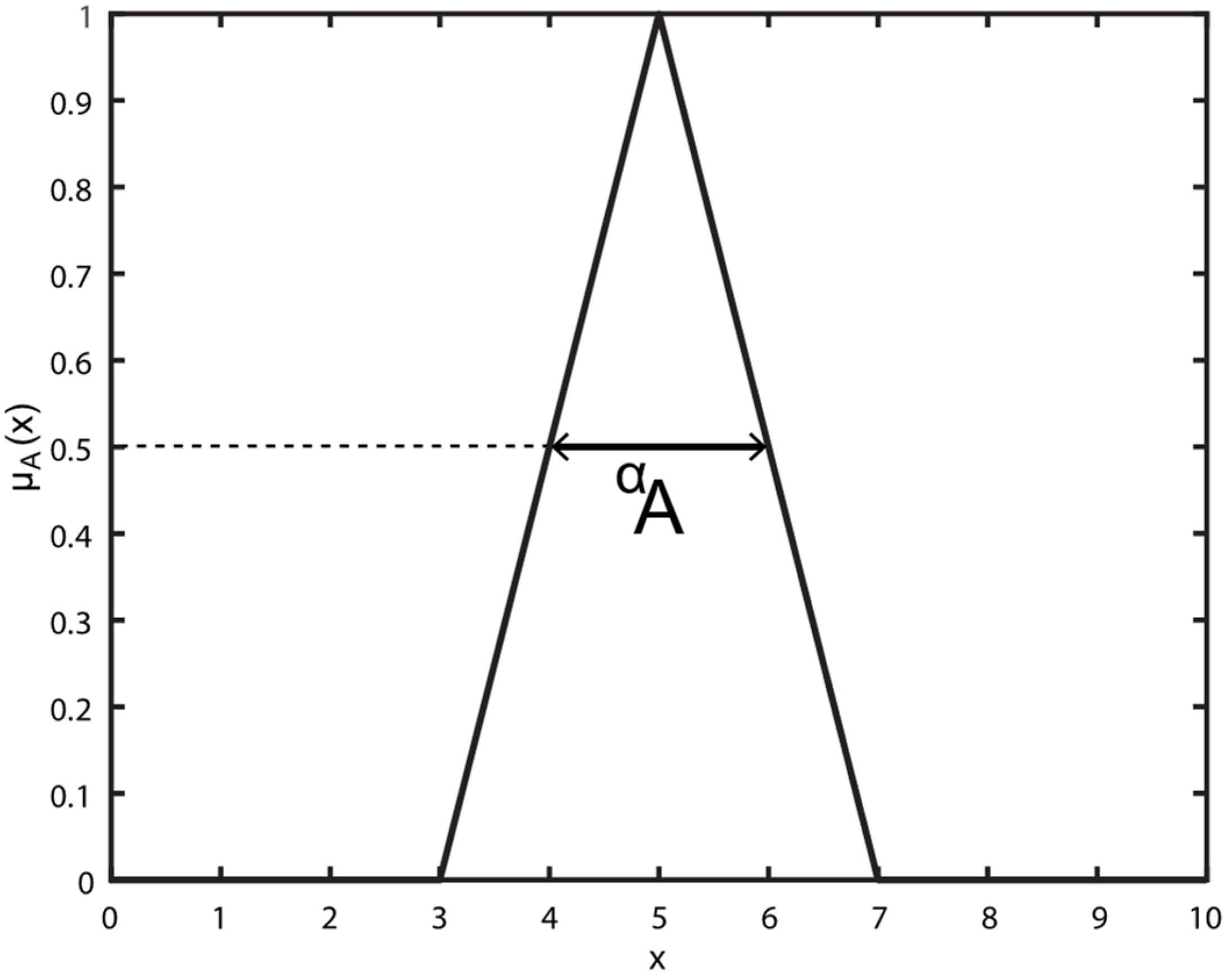
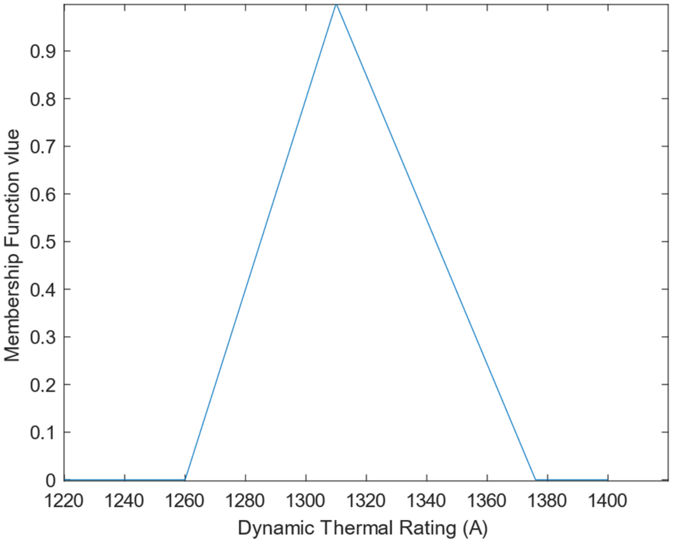
The DTR system discussed in Section 2 assumes no error in sensors used for data sampling, and the resulting values are crisp according to fuzzy theory. However, when uncertainty is considered, ranges of values can be derived, which are referred to as fuzzy numbers. In this section, the fuzzy approach is applied to the dynamic thermal rating system (DTR) and thermal aging model (TAM) to create the fuzzy-based version known as the FDTR-TAM. All of the models presented in Section 2 and Section 3 remain valid despite the addition of fuzzy theory.

4.1. Fuzzy Numbers

An important aspect of fuzzy analyses is their computational efficiency, which can be obtained by formulating the membership functions into interval calculations. Kaufman and Gupta [38] demonstrated that by composing membership functions into intervals, fuzzy analysis could reduce mathematical and computational operations. The α-cut is the composition of each fuzzy interval, and fuzzy α-cut arithmetic is applied to calculate the results associated with the α-cut. Triangular fuzzy number A and the α-cut of this fuzzy number illustrated in Figure 1 are described as the follows:

$${\mu }_A\left(x\right)=\{\begin{array}{c}0x\le a\\ \frac{x-a}{b-a}a\le x\le b\\ \frac{c-x}{c-b}b\le x\le c\\ 0x\ge c\end{array},$$

(4)

$$\forall \alpha \in \left[0,1\right]:{}^{\alpha }A=\left\{x|{\mu }_A\left(x\right)\ge \alpha \right\}=\left[{}^{\alpha }{A}_1,{}^{\alpha }{A}_2\right]=\left[{}^{\alpha }{A}_{min,}{}^{\alpha }{A}_{max,}\right],$$

(4a)

where ${\mu }_A\left(x\right)$ denotes the triangular membership function of fuzzy number A. To utilize the fuzzy outcomes constructively, various defuzzification methods are employed to convert the fuzzy results into crisp numbers, such as distance, magnitude, and centroid point [39,40,41]. The centroid point method is described as follows:

$$\overline{x}\left(A\right)=\frac{{{\displaystyle \int }}_{a_1}^{a_2}x·{\mu }_A\left(x\right)dx}{{{\displaystyle \int }}_{a_1}^{a_2}{\mu }_A\left(x\right)dx},$$

(5)

where a₁ and a₂ are the constraints for all fuzzy numbers with a nonzero membership grade.

4.2. Fuzzy DTR

The transmission line heat balance Equation (1) incorporates several meteorological data inputs, whose uncertainties are addressed by fuzzy numbers. The calculations are therefore initiated by fuzzifying the input parameters.

Weather variables such as ambient temperature $\left(T_a\right)$, wind speed $\left(V_w\right)$, and wind angle $\left(\phi \right)$ surrounding the transmission line are uncertain due to the change in time and span. In addition, uncertainties are inherent in the respective measuring instruments.

All of these inputs were thus modeled using fuzzy numbers with their membership functions, such as ${\mu }_{V_w}\left(V_w\right)$, ${\mu }_{\phi }\left(\phi \right)$, and ${\mu }_{T_a}\left(T_a\right)$. In this section, we describe how fuzzification changes Equation (1), and the following subsections explain these steps.

4.2.1. Fuzzy Model of Air Density,${}^{\alpha }{\rho }_f$

When a crisp number is added or multiplied by a fuzzy number, the membership function of the fuzzy number remains the same.

$${}^{\alpha }{T}_{film}=\left[{}^{\alpha }{T}_{fil{m}_1},{}^{\alpha }{T}_{fil{m}_2}\right]=\left[\frac{{}^{\alpha }{T}_{a_1}+T_c}{2},\frac{{}^{\alpha }{T}_{a_2}+T_c}{2}\right],$$

(6)

where $T_a$ is fuzzy. Then, the fuzzy air density, ${}^{\alpha }{\rho }_f$, is as follows:

$${}^{\alpha }{\rho }_f=\left[{}^{\alpha }{\rho }_{f_1},{}^{\alpha }{\rho }_{f_2}\right]=\left[\frac{H}{1+0.00367{}^{\alpha }{T}_{fil{m}_2}},\frac{H}{1+0.00367{}^{\alpha }{T}_{fil{m}_1}}\right],$$

(7)

such that

$$H=1.293-1.525\times {10}^{-4}{H}_e+6.379\times {10}^{-9}{H}_e{}^2.$$

(8)

4.2.2. Fuzzy Model of Air Dynamic Viscosity,${}^{\alpha }{\mu }_f$

Equation (9) contains a positive power. It can be applied directly to the membership function of${}^{\alpha }{T}_{film}$ because positive power only monotonically increases function values. Therefore, the fuzzy model of air dynamic viscosity,${}^{\alpha }{\mu }_f$, is as follows:

$${}^{\alpha }{\mu }_f=\left[{}^{\alpha }{\mu }_{f_1},{}^{\alpha }{\mu }_{f_2}\right]=\left[\begin{array}{c}\frac{1.458\times {10}^{-6}{\left({}^{\alpha }{T}_{fil{m}_1}+273\right)}^{1.5}}{{}^{\alpha }{T}_{fil{m}_2}+383.4}\\ \frac{1.458\times {10}^{-6}{\left({}^{\alpha }{T}_{fil{m}_2}+273\right)}^{1.5}}{{}^{\alpha }{T}_{fil{m}_1}+383.4}\end{array}\right],$$

(9)

4.2.3. Fuzzy Model of Air Thermal Conductivity,${}^{\alpha }{k}_f$

As mentioned above, positive powers are directly applied to${}^{\alpha }{T}_{film}$. Therefore, the fuzzy model of thermal conductivity${(}^{\alpha }{k}_f)$ is as follows:

$${}^{\alpha }{k}_f=\left[{}^{\alpha }{k}_{f_1},{}^{\alpha }{k}_{f_2}\right]=\left[\begin{array}{c}{\mathsf{{\rm Y}}}_1+{\mathsf{{\rm Y}}}_2{}^{\alpha }{T}_{fil{m}_1}-{\mathsf{{\rm Y}}}_3{}^{\alpha }{T}_{fil{m}_2}\\ {\mathsf{{\rm Y}}}_1+{\mathsf{{\rm Y}}}_2{}^{\alpha }{T}_{fil{m}_2}-{\mathsf{{\rm Y}}}_3{}^{\alpha }{T}_{fil{m}_1}\end{array}\right],$$

(10)

where ${\mathsf{{\rm Y}}}_1=2.424\times {10}^{-2}{\mathsf{{\rm Y}}}_2=7.477\times {10}^{-5}{\mathsf{{\rm Y}}}_3=4.407\times {10}^{-9}$.

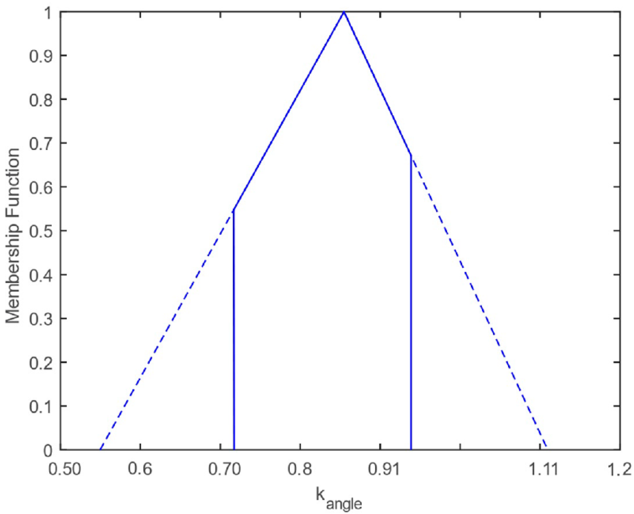
4.2.4. Fuzzy Model of Wind Direction Factor,${}^{\alpha }{k}_{angle}$

The fuzzy model of the wind direction factor${}^{\alpha }{k}_{angle}$ is as follows:

$${}^{\alpha }{k}_{angle}=\left[{}^{\alpha }{k}_{angl{e}_1},{}^{\alpha }{k}_{angl{e}_2}\right]=\left[\begin{array}{c}{x}_1+x_{2}cos\left(2{}^{\alpha }{\phi }_1\right)+x_{3}sin\left(2{}^{\alpha }{\phi }_1\right)-cos\left({}^{\alpha }{\phi }_2\right)\\ x_1+x_{2}cos\left(2{}^{\alpha }{\phi }_2\right)+x_{3}sin\left(2{}^{\alpha }{\phi }_2\right)-cos\left({}^{\alpha }{\phi }_1\right)\end{array}\right],$$

(11)

where $x_1=1.194$, $x_2=0.194$, and $x_3=0.368$.

The effect of a trigonometric function on fuzzy numbers has been discussed [38]. A wind angle range of 0° ≤ φ ≤ 90° was considered. When the crisp angle is determined without the fuzzy method by applying either the minimum or maximum constraints [0, 90°], it lies in the range of [0.38, 1], which is monotonically increasing. However, the range of final fuzzy outcomes when applying fuzzy operations does not always fall within the acceptable crisp range. To address this issue, the range of $k_{angle}$ is always compressed to the crisp acceptable range. For example, when $30°\le \phi \le 60°$ is applied to the trigonometric membership function, the calculated value of crisp $k_{angle}$ ranges between 0.74 and 0.92. However, upon applying fuzzy arithmetic, the range of k angle ranges between [0.55, 1.11]. In response, the range based on fuzzy numbers is larger than the range computed using crisp numbers. Consequently, the fuzzy $k_{angle}$ was compressed to comply with the crisp range only, as shown in Figure 2.

4.2.5. Fuzzy Model of Convective Heat Loss Rate,${}^{\alpha }{Q}_c$

The fuzzy model of convection heat loss rate, $\left({}^{\alpha }{Q}_c\right)$, is as follows:

$${}^{\alpha }{Q}_c=\left[{}^{\alpha }{Q}_{c_1},{}^{\alpha }{Q}_{c_2}\right]=\left[\begin{array}{c}max\left({}^{\alpha }{Q}_{c{H}_1},{}^{\alpha }{Q}_{c{L}_1},{}^{\alpha }{Q}_{c{N}_1}\right),\\ max\left({}^{\alpha }{Q}_{c{H}_2},{}^{\alpha }{Q}_{c{L}_2},{}^{\alpha }{Q}_{c{N}_2}\right)\end{array}\right],$$

(12)

where

$${}^{\alpha }{Q}_{cH}=\left[{}^{\alpha }{Q}_{c{H}_1},{}^{\alpha }{Q}_{c{H}_2}\right]=\left\{\begin{array}{c}\left[1.01+1.35{\left({}^{\alpha }{\gamma }_1\right)}^{0.52}\right]·{}^{\alpha }{\lambda }_1,\\ \left[1.01+1.35{\left({}^{\alpha }{\gamma }_2\right)}^{0.52}\right]·{}^{\alpha }{\lambda }_2\end{array}\right\},$$

(13a)

$${}^{\alpha }{Q}_{cL}=\left[{}^{\alpha }{Q}_{c{L}_1},{}^{\alpha }{Q}_{c{L}_2}\right]=\left\{\begin{array}{c}\left[0.754{\left({}^{\alpha }{\gamma }_1\right)}^{0.6}\right]·{}^{\alpha }{\lambda }_{1,}\\ \left[0.754{\left({}^{\alpha }{\gamma }_2\right)}^{0.6}\right]·{}^{\alpha }{\lambda }_2\end{array}\right\},$$

(13b)

$${}^{\alpha }{Q}_{cN}=\left[{}^{\alpha }{Q}_{c{N}_1},{}^{\alpha }{Q}_{c{N}_2}\right]=\left\{\begin{array}{c}\left[3.645D^{0.75}+{\left({}^{\alpha }{\rho }_{f_1}\right)}^{0.5}{\left(T_c-{}^{\alpha }{T}_{a_2}\right)}^{1.25}\right],\\ \left[3.645D^{0.75}+{\left({}^{\alpha }{\rho }_{f_2}\right)}^{0.5}{\left(T_c-{}^{\alpha }{T}_{a_1}\right)}^{1.25}\right]\end{array}\right\},$$

(13c)

such that

$${}^{\alpha }\gamma =\left[{}^{\alpha }{\gamma }_1,{}^{\alpha }{\gamma }_2\right]=\left[D\frac{{}^{\alpha }{\rho }_{f_1}{}^{\alpha }{V}_{w_1}}{{}^{\alpha }{\mu }_{f_2}},D\frac{{}^{\alpha }{\rho }_{f_2}{}^{\alpha }{V}_{w_2}}{{}^{\alpha }{\mu }_{f_1}}\right],$$

(14)

$${}^{\alpha }\lambda =\left[{}^{\alpha }{\lambda }_1,{}^{\alpha }{\lambda }_2\right]=\left[\begin{array}{c}\left({}^{\alpha }{k}_{angl{e}_1}·{}^{\alpha }{k}_{f_1}\right)·\left(T_c-{}^{\alpha }{T}_{a_2}\right),\\ \left({}^{\alpha }{k}_{angl{e}_2}·{}^{\alpha }{k}_{f_2}\right)·\left(T_c-{}^{\alpha }{T}_{a_1}\right)\end{array}\right].$$

(15)

4.2.6. Fuzzy Model of Radiation Heat Loss Rate, ${}^{\alpha }{Q}_r$

The fuzzy radiation heat loss rate $({}^{\alpha }{Q}_r)$ is as follows:

$${}^{\alpha }{Q}_r=\left[{}^{\alpha }{Q}_{r_1},{}^{\alpha }{Q}_{r_2}\right]=\left\{\begin{array}{c}17.8D\epsilon \left[{\left(\frac{T_c+273}{100}\right)}^4-{\left(\frac{{}^{\alpha }{T}_{a_2}+273}{100}\right)}^4\right],\\ 17.8D\epsilon \left[{\left(\frac{T_c+273}{100}\right)}^4-{\left(\frac{{}^{\alpha }{T}_1+273}{100}\right)}^4\right]\end{array}\right\},$$

(16)

4.2.7. Fuzzy Model of Solar Heat Gain Rate, $Q_s$

The calculation of solar heat gain rate, ($Q_s)$, begins as follows:

$$H_c=arcsin\left[cos\left(Lat\right)·cos\left(\delta \right)·cos\left(\omega \right)+sin\left(Lat\right)·sin\left(\delta \right)\right],$$

(17)

$$\delta =23.46·sin\left[\frac{284+N}{365}·360\right],$$

(18)

$$Z_c=C+arctan\left(\chi \right),$$

(19)

such that

$$\chi =\frac{sin\left(\omega \right)}{sin\left(Lat\right)·cos\left(\omega \right)-cos\left(Lat\right)·tan\left(\delta \right)},$$

(19a)

where the solar azimuth constant C is a function of the fuzzy solar hour angle, ω, and solar azimuth χ, which can be estimated from the table shown in the IEEE 738 standard.

The following is also considered:

$$\theta =arccos\left(H_c\right)·cos\left(Z_c-Z_l\right).$$

(20)

The solar heat intensity at the earth’s surface is corrected for altitude by the following:

$$Q_{se}=k_{solar}{q}_s,$$

(21)

such that

$$q_s=\left[\begin{array}{c}{u}_1+u_2\left(H_c\right)+u_3{\left(H_c\right)}^2+u_4{\left(H_c\right)}^3\\ +u_5{\left(H_c\right)}^4+u_6{\left(H_c\right)}^5+u_7{\left(H_c\right)}^6\end{array}\right],$$

(21a)

where $u_1,u_2,...u_7$ are the constants available in the IEEE standard 738 [24].

The following are also considered:

where

$$k_{solar}=s_1+s_2{H}_e+s_3{\left(H_e\right)}^2,$$

(21b)

and finally,

$$Q_s=\mathsf{\Psi }·Q_{se}·sin\left(\theta \right)·A_r.$$

(22)

4.3. Fuzzy Thermal Aging of Transmission Lines

As previously stated, the thermal aging of overhead lines is driven by the conductor temperature, which is influenced by environmental factors such as ambient temperature, wind angle, wind speed, and solar hourly angle. The uncertainties associated with these variables are considered fuzzy numbers in Section 4.

Among the different types of conductors used in high-voltage transmission lines, the aluminum conductor steel reinforced (ACSR) type is now employed globally for technical and economic reasons. Therefore, the fuzzy thermal aging model was derived only on the basis of ACSR in this study.

Table 1. Physical and constructional properties of typical ACSR.

Codeword	Cross-Sectional Area		Stranding		Rated Strength of Steel Core Coating, N
	${\mathit{A}}_{\mathit{a}\mathit{l}}$ ${\mathbf{m}\mathbf{m}}^2$	${\mathit{A}}_{\mathit{s}\mathit{t}}$ ${\mathbf{m}\mathbf{m}}^2$	Number ${\mathit{\eta }}_{\mathit{a}\mathit{l}}/{\mathit{\eta }}_{\mathit{s}\mathit{l}}$	Diameter ${\mathit{d}}_{\mathit{a}\mathit{l}}/{\mathit{d}}_{\mathit{s}\mathit{t}}$ $\mathbf{m}\mathbf{m}$
Kiwi	1098.2	47.5	72/7	4.45/2.97	223,000
Cardinal	483.3	62.6	54/7	3.43/3.43	150,000
Curlew	523.4	67.8	54/7	3.51/3.51	157,000
Drake	403.0	65.6	26/7	4.44/3.45	135,000
Heron	253.4	59.1	30/7	3.45/3.45	118,000
Saguenay	561.2	189.5	36/19	4.50/3.60	298,000

lists the physical and structural properties of several ACSR variants according to the American Society for Testing and Materials (ASTM) B 354-98 standard [42].

As mentioned above, positive powers were directly applied to $\left({}^{\alpha }{T}_{film}\right)$. Therefore, the fuzzy model of creep $\left({}^{\alpha }{\epsilon }_c\right)$ is as follows:

$${}^{\alpha }{\epsilon }_c=\left[{}^{\alpha }{\epsilon }_{c_1},{}^{\alpha }{\epsilon }_{c_2}\right]=\left[\begin{array}{c}0.24{\left(\%{}^{\alpha }R{S}_1\right)}^{1.3}{}^{\alpha }{T}_{c_1}{t}^{0.16},\\ 0.24{\left(\%{}^{\alpha }R{S}_2\right)}^{1.3}{}^{\alpha }{T}_{c_2}{t}^{0.16}\end{array}\right],$$

(23)

where %${}^{\alpha }RS=\left[{\%}^{\alpha }R{S}_1,{\%}^{\alpha }R{S}_2\right]$ is the remaining percentage strength of the conductor, and t is the number of hours operating at $\left({}^{\alpha }{T}_c\right)$.

The %RS is determined as follows [34]:

$${}^{\alpha }RS=\left[{}^{\alpha }R{S}_1,{}^{\alpha }R{S}_2\right]=\left[\begin{array}{c}{}^{\alpha }R{S}_{a{l}_1}\left(\frac{ST{R}_{al}}{ST{R}_T}\right)+109\left(\frac{ST{R}_{st}}{ST{R}_T}\right)\\ {}^{\alpha }R{S}_{a{l}_2}\left(\frac{ST{R}_{al}}{ST{R}_T}\right)+109\left(\frac{ST{R}_{st}}{ST{R}_T}\right)\end{array}\right],$$

(24)

such that

$${}^{\alpha }R{S}_{al}=\left[{}^{\alpha }R{S}_{al}{}_1,{}^{\alpha }R{S}_{al}{}_2\right]=\left[\begin{array}{c}\{\begin{array}{c}{}^{\alpha }{\beta }_1{t}^{\varphi }if{}^{\alpha }{\beta }_1⋖100\\ 100t^{\varphi }otherwise\end{array},\\ \{\begin{array}{c}{}^{\alpha }{\beta }_2{t}^{\varphi }if{}^{\alpha }{\beta }_2⋖100\\ 100t^{\varphi }otherwise\end{array}\end{array}\right],$$

(25)

where

$$ST{R}_{al}=\pi {\eta }_{al}{d}_{al}{}^2{S}_{al}{k}_{al}/4,$$

(26a)

$$ST{R}_{sl}=\pi {\eta }_{sl}{d}_{sl}{}^2{S}_{sl}^{1\%}{k}_{sl}/4,$$

(26b)

$$ST{R}_T=ST{R}_{al}+ST{R}_{sl}.$$

(26c)

$ST{R}_{al}$ and $ST{R}_{sl}$ in (26a,b) are the strengths of the ACSR’s aluminum and steel strands, respectively, and $ST{R}_T$ is the total strength of the ACSR. $({}^{\alpha }\beta$) and $\left({}^{\alpha }\varphi \right)$ in (25) were calculated as follows:

$${}^{\alpha }\beta =\left[{}^{\alpha }{\beta }_1,{}^{\alpha }{\beta }_2\right]=\left[\begin{array}{c}134-0.24{}^{\alpha }{T}_{c_1,}\\ 134-0.24{}^{\alpha }{T}_{c_2}\end{array}\right],$$

(27)

$${}^{\alpha }\varphi =\left[{}^{\alpha }{\varphi }_1,{}^{\alpha }{\varphi }_2\right]=\left[\begin{array}{c}\left(0.241-0.00254{}^{\alpha }{T}_{c_1}\right)/d_{al},\\ \left(0.241-0.00254{}^{\alpha }{T}_{c_2}\right)/d_{al}\end{array}\right],$$

(28)

where $d_{al}$ is the diameter of the aluminum strand, and $d_{sl}$ is the diameter of the steel strand; the remaining variables in (26a) and (26b), such as ${\eta }_{al}$ and ${\eta }_{sl}$, are the number of strands of aluminum and steel provided in Table 1 [43]. $S_{al}$ is the average breaking stress of aluminum given in

Table 2. Breaking tensile stress and diameter tolerance of aluminum wires.

Nominal Diameter mm	Breaking Stress, MPa		Permissible Variations from Nominal Diameter
	Average/Lot	Individual Tests
1.26–1.50	200	185	$\pm 0.03$
1.51–2.00	195	185
2.01–2.25	190	180
2.26–2.50	185	175
2.51–2.75	180	170
2.76–3.00	175	165
3.01–3.75	170	160	$\pm 1\%$
3.76–5.25	165	160
5.26–6.50	160	155

[44], and $S_{sl}^{1\%}$ is the average breaking stress of steel’s core at 1% extension given in

Table 3. Tensile requirement and diameter tolerance of zinc-coated, steel-core wires.

Nominal Diameter mm	Breaking Stress, MPa			Permissible Variations from Nominal Diameter
	Coating Class A	Coating Class A	Coating Class A
1.60–2.30	1310	1240	1170	+0.04; −0.03
2.31–3.05	1280	1210	1140	$\pm 0.05$
3.06–3.60	1240	1170	1100	+0.08; −0.05
3.61–4.80	1170	1100	1070	+0.10; −0.08

[45], where $k_{al}$ and $k_{sl}$ are the aluminum and steel reduction factors, respectively [46]. All of the variables are discussed in this study, except for their SI units.

The tensile strength of an ACSR is defined as the highest load per unit of cross-sectional area that a tensioned conductor can withstand during a rupture test. Thus, an ACSR conductor’s loss of tensile strength (LOTS) is expressed as a percentage and computed as follows:

$${}^{\alpha }LOTS=\left[{}^{\alpha }LOT{S}_1,{}^{\alpha }LOT{S}_2\right]=\left[100\%-{}^{\alpha }R{S}_1,100\%-{}^{\alpha }R{S}_2\right].$$

(29)

The LOTS of the ACSR conductor is measured by considering ${}^{\alpha }Tc$, which is obtained from the fuzzy dynamic thermal model presented in Section 4.3. When determining the economic cost of conductors based on the LOTS, the following factors are considered: length L (in meters) of the transmission line on which the conductor is used, weight-to-length ratio ${\mho }_{w:L}$ (kg/m), and cost-to-weight ratio ${\mho }_{c:w}$ (USD/kg), as follows:

$${}^{\alpha }Cos{t}_{LOTS}=\left[{}^{\alpha }Cos{t}_{LOTS1},{}^{\alpha }Cos{t}_{LOTS2}\right]=\left[\begin{array}{c}{}^{\alpha }LOTS\times \left(L\times {\mho }_{w:L}\times {\mho }_{c:w}\right)\left[\frac{USD}{100\%}\right],\\ {}^{\alpha }LOTS\times \left(L\times {\mho }_{w:L}\times {\mho }_{c:w}\right)\left[\frac{USD}{100\%}\right]\end{array}\right].$$

(30)

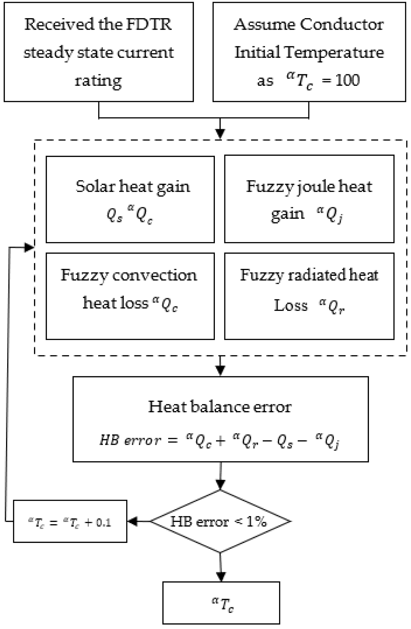
4.4. Conductor Temperature

The solution to ${}^{\alpha }{\epsilon }_c$ requires determining ${}^{\alpha }{\mathrm{T}}_c$. To perform this function, we refer to the IEEE 738 standard [24], as shown in the following:

$${}^{\alpha }{Q}_c\left({}^{\alpha }{T}_c,{}^{\alpha }{T}_a,{}^{\alpha }{V}_w,{}^{\alpha }\phi \right)+{}^{\alpha }{Q}_r\left({}^{\alpha }{T}_a,{}^{\alpha }{T}_c\right)=Q_s\left(\omega \right)+{}^{\alpha }{Q}_j\left[I,R\left({}^{\alpha }{T}_c\right)\right],$$

(31)

where

$${}^{\alpha }{Q}_j=\left[{}^{\alpha }{I}^2\mathrm{R}\left({}^{\alpha }{T}_c\right)\right].$$

(31a)

Equation (31a) is the modified fuzzy heat balance equation describing the heat exchanges of overhead lines due to uncertain meteorological conditions. Owing to the non-linear state of this equation with the data of ${}^{\alpha }\mathrm{I}$ and all of the remaining parameters being the same, the equation is applied backwards to compute the ${}^{\alpha }{T}_c$ that satisfies the fuzzy heat balance Equation (31a). ${}^{\alpha }{T}_c$ was initially set at 100 °C, and in each iteration, ${}^{\alpha }{T}_c$ was increased or decreased by 1 °C, and (31a) was computed. This back-calculation process was ended when the consecutive heat balance (HB) error was less than 1%, as twenty years of hourly weather data were used in the analysis.

The illustration of this process is as shown in Figure 3.

5. Sensitivity Analysis of Meteorological Parameters and Conductor Properties

The static thermal rating (STR) continues to be the primary method used by overhead transmission lines to determine the current carrying capacity.

Table 4. Limits of the static rating.

Parameter	Value
Wind speed (m/s)	0.61
Wind direction angle ($°$)	90
Ambient temperature ($°\mathrm{C}$)	40
Solar intensity (w/m2)	1000
Radiation factor	0.5
Absorption factor	0.5
Maximum operating temperature ($°\mathrm{C}$)	1000

outlines the limits of the static rating. Unlike STR, DTR assesses the current carrying capacity using actual meteorological parameters. Thus, the line capacity can be increased significantly.

The STR calculated at T_a = 40 $°\mathrm{C}$ and V_w = 0.61 is 768A, and following that, the current-carrying capacity was evaluated according to the variation in meteorological conditions.

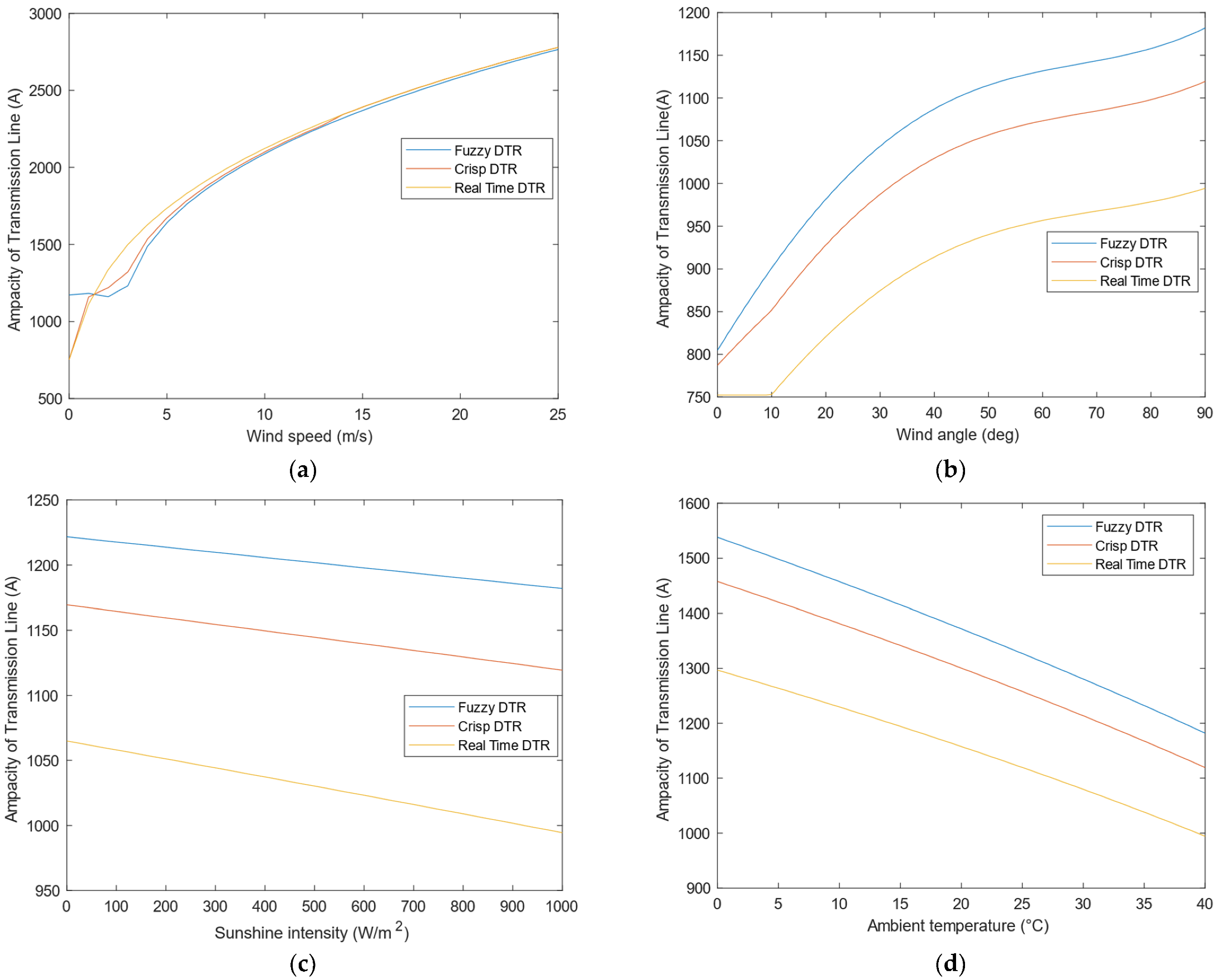
5.1. Impact of Wind Speed on the Ampacity of Overhead Transmission Line

Convection cooling is affected by wind speed. As long as the other parameters remain constant, the range of the wind speed change is assumed to be 0–25 m/s. Figure 4a illustrates the effect of wind speed on the ampacity. As seen in Figure 4a, in the wind speed section of 0–4 m/s, as the wind speed increases, a small difference is observed in the fuzzy ampacity from 1172 A to 1232 A; however, the crisp ampacity rating increases rapidly from 752 A to 1321 A. Relative to the wind speed of 0 m/s, the carrying capacity increased by 5% and 75.6% for fuzzy and crisp ratings, while in the 4–25 m/s wind speed section, fuzzy and crisp ampacity increased from 1232 A up to 2765 A and 1321 A up to 2779 A, respectively. Compared with the wind speed of 0–4 m/s, the ampacity increased by 124% and 108%, respectively. The impact of wind speed increased as the wind speed increased. Consequently, the wind speed has a great impact on the ampacity of the transmission line.

5.2. Impact of Wind Angle on the Ampacity of Overhead Transmission Line

The wind direction is a determining factor for the convective cooling of overhead lines. While keeping the other environmental conditions constant, the impact of the wind direction angle (0°–90°) on the ampacity of the transmission line is illustrated in Figure 4b. In the wind angle range of 0°–45°, with the increase in the angle, the crisp and fuzzy ampacity of the line increased from 787A up to 1041 A and 804 A up to 1100 A, respectively.

Compared with the wind angle of 0°, the ampacity increased by 32.27% and 36.81%. In the wind angle range of 45°–90°, as the angle increased, the ampacity increased from 1041 A to 1119 A and 1100 A to 1181 A. The ampacity increased by 7.49% and 7.36% with respect to the wind angle range of 0°–45°. Consequently, the wind angle has a great impact on the ampacity of the transmission line.

5.3. Impact of Solar Intensity on the Ampacity of Overhead Transmission Line

Among the factors affecting the ampacity of overhead transmission lines, solar intensity is the one that affects the solar absorption of overhead lines. By keeping the other environmental parameters constant and assuming a solar intensity range of 0–1000 w/m², the impact of solar intensity on ampacity is shown in Figure 4c.

The impact of solar intensity on the ampacity decreases almost linearly. The solar absorption of the transmission line increased as the intensity of the sunlight increased, and the crisp and fuzzy ampacity of the line decreased from 1169 A to 1119 A and 1221.4 A to 1181 A, respectively. The ampacity of the line dropped by 4.2% and 3.2% compared with a solar intensity of 0 w/m². Thus, the solar intensity has a relatively small impact on the ampacity of the transmission line.

5.4. Impact of Ambient Temperature on the Ampacity of Overhead Transmission Line

The ambient temperature surrounding the overhead transmission line is the influencing factor on the radiation dissipation. Keeping the other environmental conditions constant, the impact of the ambient temperature ranging from 0 °C–40 °C on the ampacity is shown in Figure 4d.

The impact of ambient temperature on the current carrying capacity of the line decreases almost linearly. The difference between the conductor temperature and the ambient temperature decreased as the ambient temperature rose from 0 °C to 40 °C. Therefore, radiation cooling was reduced. Thus, the crisp and fuzzy ampacity of the line was reduced from 1457 A to 1118 A and 1538 A to 1180 A, respectively. The ampacity of the line dropped by 23.26% and 22.27% compared with the temperature of 0 °C. Hence, the ambient temperature also has a great impact on the ampacity of the transmission line.

5.5. Impact of Emissivity on the Ampacity of Overhead Transmission Line

The emissivity is also one of the factors influencing the capacity of the overhead transmission line. The emissivity of the overhead conductor surface affects the amount of heat radiation from the conductor, as described in Equation (16). In stranded conductors, each strand of a conductor radiates heat in all directions. The emissivity factor of a new conductor is low, around 0.23, whereas that of an aged conductor is much higher at approximately 0.91. Thus, keeping the other environmental conditions constant, the impact of the emissivity constant (0.23 to 0.91) on the ampacity of the transmission line is illustrated in Figure 5a.

The impact of emissivity on the current carrying capacity of the line increases almost linearly. As the emissivity constant value increased, the crisp and fuzzy ampacity of the line increased from 1069 A to 1192 A and 1114 A to 1240 A, respectively. The ampacity of the line increased by 11.05% and 11.31% compared with the emissivity constant of 0.23. The emissivity constant has a relatively small impact on the ampacity of the transmission line at a higher current carrying limit and has a great impact at a lower current-carrying limit.

5.6. Impact of Solar Absorption on the Ampacity of Overhead Transmission Line

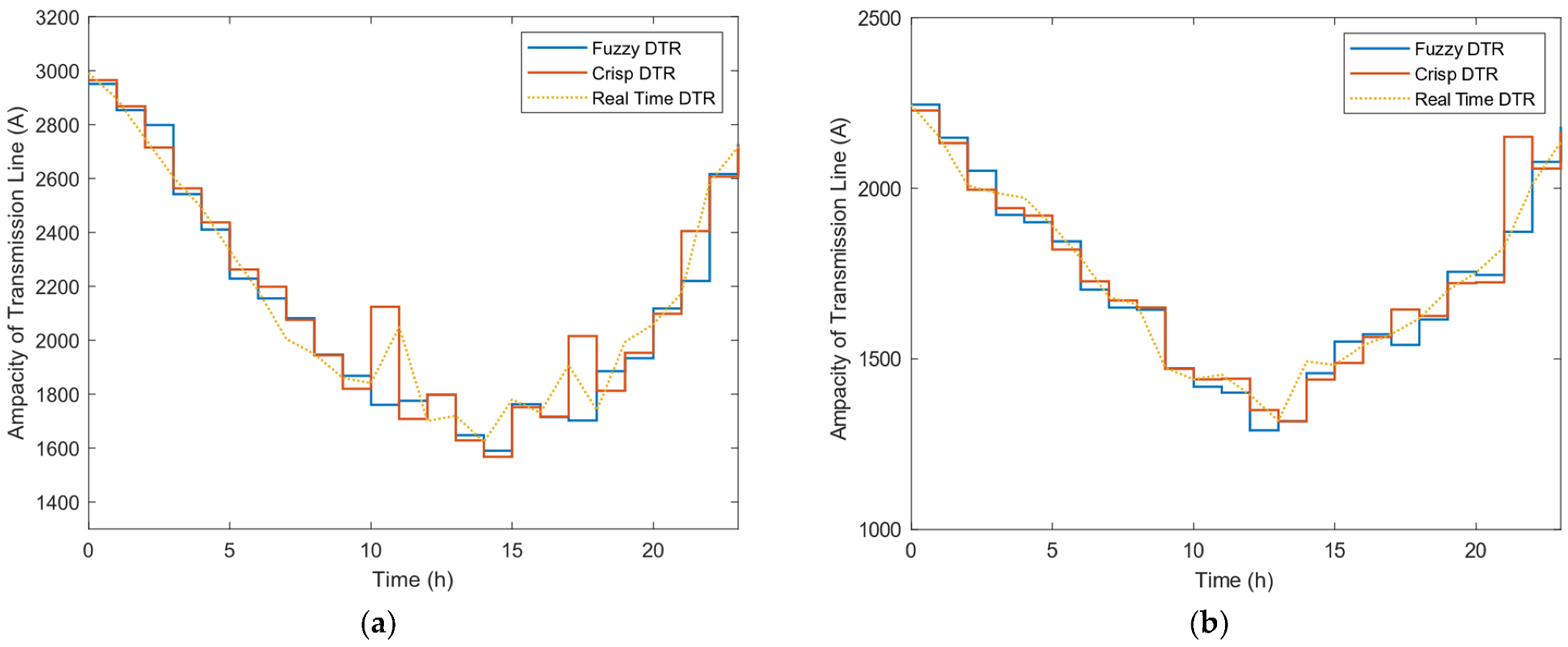
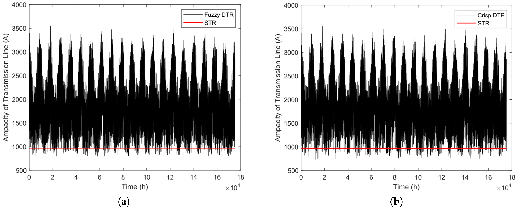
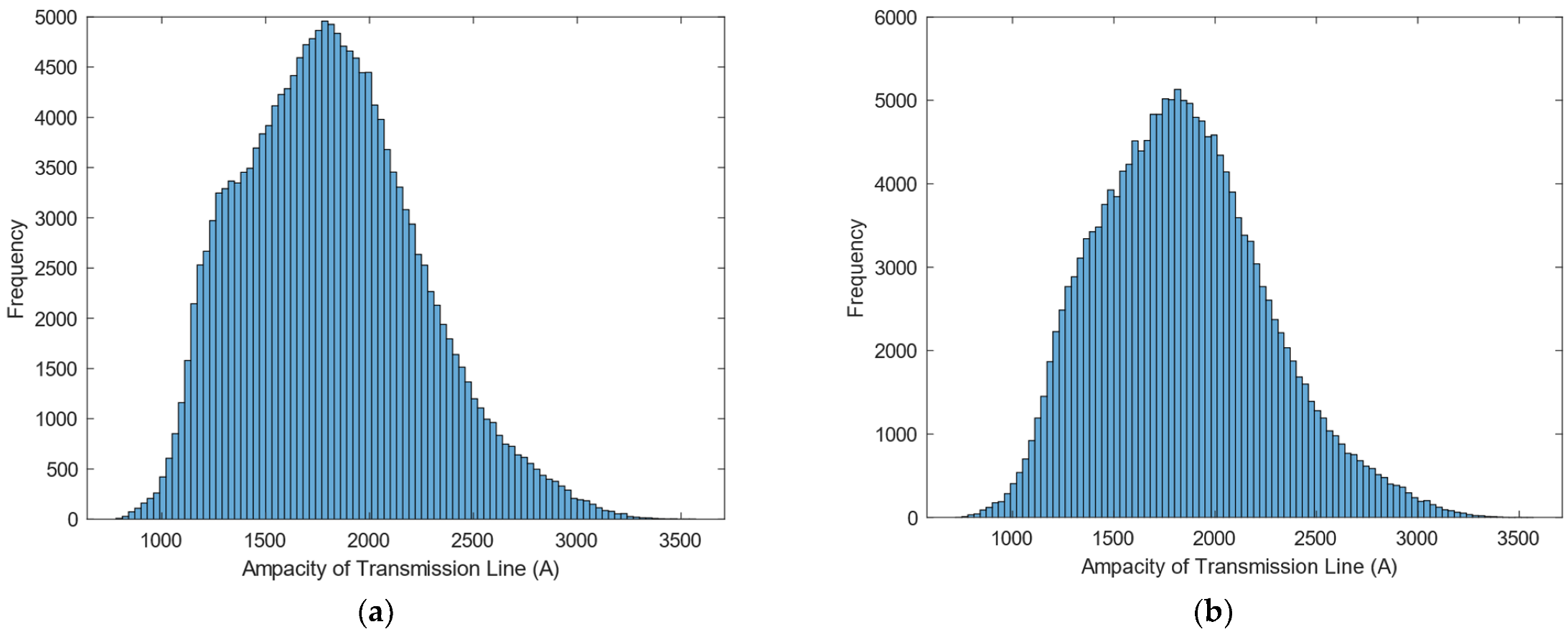
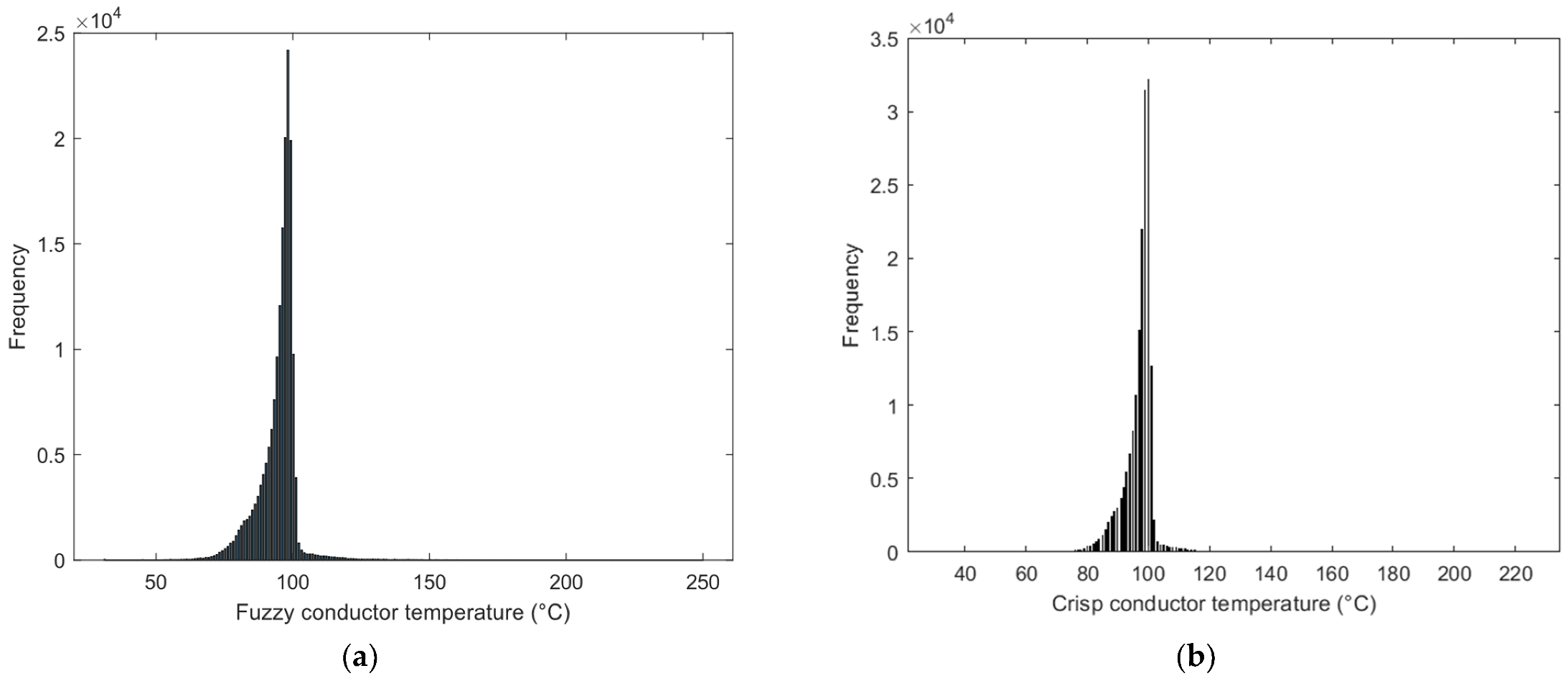
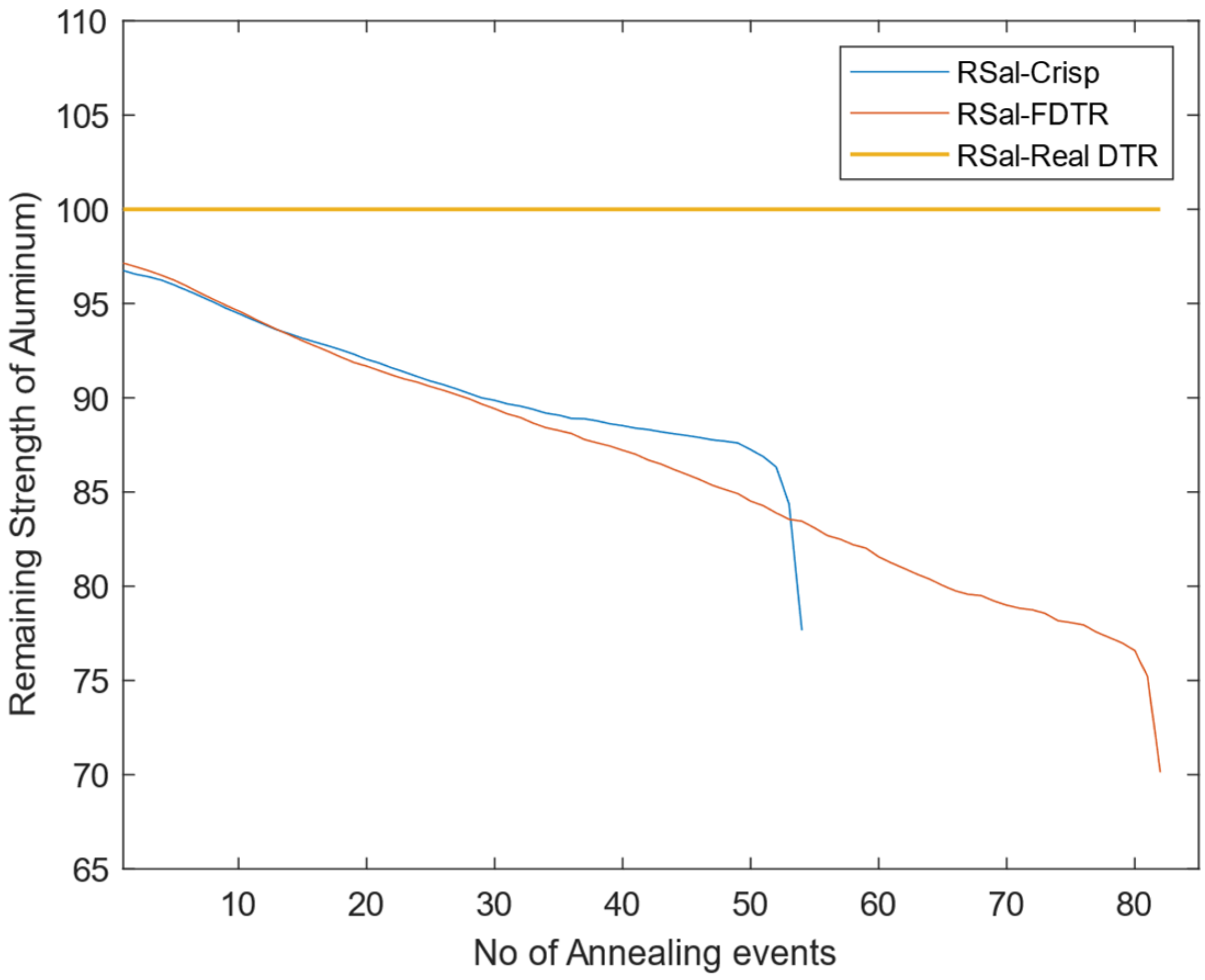
The solar absorption factor directly influences the capacity of the overhead transmission line. The solar absorption factor has a direct impact on the heat gain rate (Qs), as described in (22). In contrast to conductor emissivity, solar absorption has the opposite impact on capacity. In stranded conductors, each strand of a conductor radiates heat in all directions. Assuming that the solar absorption factor varies between 0.23 and 0.91 while keeping the other environmental conditions constant, the impact of the solar absorption factor on the ampacity of the transmission line is illustrated in Figure 6.

The impact of the solar absorption factor on the current carrying capacity of the line decreases almost linearly. As the solar absorption factor value increased, the crisp and fuzzy ampacity of the line decreased from 1146 A to 1077 A and 1203 A to 1149 A, respectively. The ampacity of the line decreased by 6.02% and 4.48% compared with a solar absorption factor of 0.23. Consequently, the solar absorption factor has a relatively small impact on the ampacity of the transmission line.

6. Case Studied

To illustrate the application of the fuzzy thermal aging analysis on a real-time power transmission system, a 150 km sample transmission line is considered. The conductor is assumed to be a Drake ACSR conductor, and the properties of the conductor are provided in Table 1, Table 2 and Table 3, with a weight-to-length ratio w:L of 1.6266 kg/m and a cost-to-weight ratio c:w of USD 1.86/kg [47]. Given these values, the cost of 100% conductor annealing is approximately USD 302 K based on (30). The historical wind speed data along the power transmission line were derived from the British Atmospheric Data Centre (BADC) [48] website for the period from 1991 to 2010, provided in 1 h time resolutions. The historical weather data were used to back-calculate the conductor temperature T_c following the fuzzy dynamic thermal model presented in Section 4.4. The maximum line loading was arbitrarily set at 3500 A, along with a transmission capacity reserve of 10% [49]. The conductor temperature T_c was subsequently used to determine the conductor’s Lots, annealing, and economic value, as given in Section 4.3.

To emulate the real operation of a transmission system, the first part of the study considered the fuzzy dynamic thermal rating (FDTR) of the transmission line using the methodology described in Section 4. The meteorological data obtained from (BADC) were used for FDTR. Weather data are highly uncertain due to the absence of sample stations along the transmission lines, measurement inaccuracies, and unpredictable weather changes. The measurement errors associated with ambient temperature (T_a), wind speed (V_w), and wind angle (φ) were assumed to be 5 times those in [29]. Thus, the triangle membership function was used to create the membership function for all parameters. The membership function’s domain is equal to the range of possible values for the relevant parameter. Each parameter’s membership function was created on the basis of its changes throughout the preceding period.

The dynamic ratings of the transmission line were calculated by applying the fuzzy and crisp approaches, and the obtained results were compared with the real-time dynamic rating. Figure 6a,b illustrate the fuzzy DTR, crisp DTR, and real-time DTR of the line for 24 h in winter and summer. Figure 7 shows the fuzzy dynamic rating on 30 June 2010 at 11 am. It shows that the possible line rating lies between 1260 and 1376 A, which is higher than the static rating. Power utilities can use 1260 A or 1376 as the line’s rating or use the defuzzified number.

We recall that the static rating of the line is 768 A from Section 5. The dynamic rating of the line is always higher than its static rating, as shown in the figures. During certain periods of time, DTR is nearly twice as high as the static rating. Thus, adopting the dynamic rating is critical for alleviating the congestion of the transmission system. As shown in Figure 6a,b, the fuzzy model considers the changes in parameters during each period and generates a value close to the average during that time period. However, in crisp DTR, it is demonstrated that the estimated DTR is excessively high at some points, i.e., the 20th hour in Figure 6a and the 10th and 17th hours in Figure 6b. Thus, the fuzzy model obviously performs better than crisp analysis, as it considers all of the changes in the line rating for each time interval.

The ampacity of the transmission line was calculated using the fuzzy and crisp method, corresponding to 1 h intervals for the 20-year meteorological data. Figure 8 shows the scatter diagram. The current carrying capacity is higher in winter than in summer, which is consistent with meteorological parameters, such as low ambient temperature in winter and high ambient temperature in summer.

The average current carrying capacity of the fuzzy rating is 1818, and the crisp rating is 1876. The scatter plots show that very few data points are below the static rating of 768 A, which verifies that DTR can significantly improve the utilization of available transmission capacity. As shown in Figure 9a, the frequency sum of data greater than 1190 A is 95%, and the frequency sum of data greater than 1306 A is 90% in the fuzzy rating. Therefore, when the current value is 1190 A and 1306 A, the operational risks are 5% and 10%, respectively. The dynamic carrying capacity improved by 54.6% and 75%, respectively, compared with STR. As shown in Figure 9b, the frequency sum of data greater than 1210 A is 95%, and the frequency sum of data greater than 1349 A is 90% in the crisp rating. Therefore, when the current values are 1210 A and 1349 A, the operational risks are 5% and 10%, respectively. The dynamic carrying capacity improved by 57.56% and 75.65%, respectively, compared with STR. The findings indicate that STR is a conservative method, whereas DTR can substantially improve the usage of available transmission capacity.

Drake ACSRs are conductors that can withstand increased demand and high temperatures of up to 250 °C. To the best of the authors’ knowledge, the effect of high temperature on overhead transmission lines has been studied only in emergency conditions. In this study, we analyzed the thermal behavior of overhead transmission lines on the basis of the dynamic thermal rating. Thermal stress is largely influenced by weather conditions. Weather is the most challenging aspect of monitoring the overhead conductor temperature. The temperatures of conductors vary in each span length due to climate change. Thus, the range of conductor temperatures may reach or exceed their limit under complex terrain conditions.

All of the weather sensors have their own measuring errors, and determining the error is difficult due to the high variability of meteorological parameters. In the first set of studies, the fuzzy model was validated to consider the fluctuation of parameters during each period and outperformed the crisp and real-time DTR method according to the above method, corresponding to 1 h time intervals for 20 years based on real-time meteorological data. The ampacity of the transmission line was calculated assuming that the line studied will be in service for 20 years. Section 4.1 presents the real-time weather data used to back-calculate the conductor temperature T_c in accordance with the dynamic thermal model.

Figure 10a,b show a frequency histogram of conductor temperatures for a period of twenty years for fuzzy and crisp ratings. The exposure times for different temperatures over twenty years were calculated on the basis of the histogram.

Table 5. Exposure time according to the frequency of conductor temperatures for fuzzy dynamic rating over a twenty-year period.

Temp °C	Time (h)	Temp °C	Time (h)	Temp °C	Time (h)	Temp °C	Time (h)	Temp °C	Time (h)	Temp °C	Time (h)	Temp °C	Time (h)
101	3907	113	159	125	41	137	31	149	9	161	7	173	2
102	810	114	139	126	34	138	17	150	15	162	6	174	4
103	413	115	133	127	35	139	15	151	9	163	6	175	1
104	351	116	113	128	33	140	19	152	13	164	5	177	1
105	290	117	104	129	40	141	17	153	11	165	6	178	3
106	289	118	106	130	33	142	24	154	3	166	5	180	2
107	291	119	93	131	36	143	15	155	10	167	3	188	1
108	243	120	57	132	24	144	18	156	11	168	1	193	1
109	224	121	66	133	35	145	15	167	5	169	4	213	1
110	184	122	57	134	29	146	14	168	7	170	3	250	1
111	191	123	49	135	16	147	15	159	4	171	2
112	180	124	34	136	16	148	10	160	10	172	1

and

Table 6. Exposure time according to the frequency of conductor temperatures for crisp dynamic rating over a twenty-year period.

Temp °C	Time (h)	Temp °C	Time (h)	Temp °C	Time (h)	Temp °C	Time (h)	Temp °C	Time (h)	Temp °C	Time (h)	Temp °C	Time (h)
101	12,653	109	268	117	58	125	36	133	14	141	6	151	1
102	2167	110	210	118	57	126	26	134	6	142	3	156	2
103	660	111	192	119	53	127	29	135	8	143	4	163	1
104	472	112	170	120	60	128	30	136	12	1441	3	168	1
105	453	113	146	121	40	129	28	137	1	146	2	187	1
106	381	114	101	122	48	130	14	138	6	147	2	225	1
107	322	115	92	123	40	131	19	139	8	148	2
108	290	116	70	124	38	132	11	140	5	149	1

summarize the detailed histograms for fuzzy and crisp temperatures over 100 °C for aluminum and are illustrated in Figure 10c,d.

The conductor loss of tensile strength due to annealing at a certain temperature was calculated according to its exposure time. The combined loss of tensile strength of the conductor was determined by considering the physical properties of the conductor. The loss of strength values of the aluminum strands of the conductor for fuzzy and crisp dynamic ratings are 30.05% and 22.16%, respectively. The Drake conductor is a composite conductor with a steel core. Therefore, its total loss of tensile strength is substantially reduced. The total loss values of tensile strength in a composite conductor for fuzzy and crisp ratings are 9.37% and 4.71%, respectively. The loss of strength increases when the conductor’s exposure time to high temperature increase, as illustrated in Figure 11.

Table 7. Loss of tensile strength in aluminum strands and in the complete conductor over a twenty-year period.

Thermal Effect of Fuzzy Dynamic Rating				Thermal Effect of Crisp Rating
Range of Temperature $°\mathbf{C}$	Percentage of Exposure Time	Loss of Aluminum Strands Strength (%)	Loss of Tensile Strength of Conductor (%)	Range of Temperature $°\mathbf{C}$	Percentage of Exposure Time	Loss of Aluminum Strands Strength (%)	Loss of Tensile Strength of Conductor (%)
100–125	92.32	9.51	0	100–125	98.67	9.20	0
126–150	6.06	6.30	1.81	126–150	1.3	3.56	0.51
151–175	1.61	6.19	4.53	151–250	0.03	9.40	4.20
175–250	0.01	8.05	3.396	Total		22.16	4.71
Total		30.05	9.736

illustrates the loss of tensile strength for fuzzy and crisp ratings for a duration of 20 years. The resulting conductor loss of tensile strength will affect the service life of transmission lines. Furthermore, the calculated creep values under these conditions are 540.03 and 441.17 micro-meters/meter for fuzzy and crisp ratings, and the economic costs are 2.9385 × 10⁴ and 1.428 × 10⁴, respectively.

However, no loss of strength occurred for real-time DTR, as it does not consider the uncertainties of weather data. Fuzzy and crisp ratings comparatively consider variations in weather data and provide compressive information regarding the thermal analysis of the transmission line. Hence, this method provides an opportunity to mitigate the operational risk to the transmission line.

Conductors with higher-than-normal temperatures generate unwanted thermal stress and have a negative effect on their thermal behavior, reducing their strength, affecting their vertical ground clearance, and hastening their annealing process. As the conductor is operated over a long period of time, both its performance and service life deteriorate. Hence, momentarily raising the conductor temperature limit can possibly meet the need for higher line ampacity depending on the load demand. However, its operational risk must first be assessed and determined to ensure that it is within the permissible limit.

7. Conclusions

This study presents a fuzzy thermal aging framework for overhead transmission lines equipped with the DTR system. Based on the transmission conductor characteristics, load, and weather data, the method determines a time series of conductor temperatures and corresponding thermal aging. Moreover, the impact of uncertain meteorological parameters and conductor physical properties on the ampacity of transmission lines is discussed. The method presented in this paper helps eliminate network congestion because it considers the real-time load, actual physical properties, and aging of the conductor. It enables other renewable integrations to achieve a low-carbon network. Following the aging assessment of conductors performed based on real-time meteorological data, the results indicate that thermal aging and transmission capacity are strongly correlated, and the framework is robust such that uncertain variations in meteorological parameters are also addressed adequately. This information is crucial for line inspections, maintenance, and reconductoring procedures within transmission networks, as well as effective transmission asset management.

References

1. Lai, C.M.; Teh, J. Comprehensive Review of the Dynamic Thermal Rating System for Sustainable Electrical Power Systems. Energy Rep. 2022, 8, 3263–3288. [Google Scholar] [CrossRef]
2. Metwaly, M.K.; Teh, J. Optimum Network Ageing and Battery Sizing for Improved Wind Penetration and Reliability. IEEE Access 2020, 8, 118603–118611. [Google Scholar] [CrossRef]
3. Teh, J.; Lai, C.M.; Muhamad, N.A.; Ooi, C.A.; Cheng, Y.H.; Zainuri, M.A.A.M.; Ishak, M.K. Prospects of Using the Dynamic Thermal Rating System for Reliable Electrical Networks: A Review. IEEE Access 2018, 6, 26765–26778. [Google Scholar] [CrossRef]
4. Teh, J.; Cotton, I. Risk Informed Design Modification of Dynamic Thermal Rating System. IET Gener. Transm. Distrib. 2015, 9, 2697–2704. [Google Scholar] [CrossRef]
5. Lai, C.M.; Teh, J. Network Topology Optimisation Based on Dynamic Thermal Rating and Battery Storage Systems for Improved Wind Penetration and Reliability. Appl. Energy 2022, 305, 117837. [Google Scholar] [CrossRef]
6. Teh, J.; Lai, C.M. Reliability Impacts of the Dynamic Thermal Rating and Battery Energy Storage Systems on Wind-Integrated Power Networks. Sustain. Energy Grids Netw. 2019, 20, 100268. [Google Scholar] [CrossRef]
7. Daminov, I.; Rigo-Mariani, R.; Caire, R.; Prokhorov, A.; Alvarez-Herault, M.-C. Demand Response Coupled with Dynamic Thermal Rating for Increased Transformer Reserve and Lifetime. Energies 2021, 14, 1378. [Google Scholar] [CrossRef]
8. Metwaly, M.K.; Teh, J. Probabilistic Peak Demand Matching by Battery Energy Storage alongside Dynamic Thermal Ratings and Demand Response for Enhanced Network Reliability. IEEE Access 2020, 8, 181547–181559. [Google Scholar] [CrossRef]
9. Khoo, W.C.; Teh, J.; Lai, C.M. Demand Response and Dynamic Line Ratings for Optimum Power Network Reliability and Ageing. IEEE Access 2020, 8, 175319–175328. [Google Scholar] [CrossRef]
10. Teh, J.; Cotton, I. Reliability Impact of Dynamic Thermal Rating System in Wind Power Integrated Network. IEEE Trans. Reliab. 2016, 65, 1081–1089. [Google Scholar] [CrossRef]
11. Teh, J.; Lai, C.M.; Cheng, Y.H. Improving the Penetration of Wind Power with Dynamic Thermal Rating System, Static VAR Compensator and Multi-Objective Genetic Algorithm. Energies 2018, 11, 815. [Google Scholar] [CrossRef] [Green Version]
12. Teh, J.; Lai, C.; Cheng, Y. Impact of the Real-Time Thermal Loading on the Bulk Electric System Reliability. IEEE Xplore 2017, 66, 1110–1119. [Google Scholar] [CrossRef]
13. Musilek, P.; Heckenbergerova, J.; Bhuiyan, M.M.I. Spatial Analysis of Thermal Aging of Overhead Transmission Conductors. IEEE Trans. Power Deliv. 2012, 27, 1196–1204. [Google Scholar] [CrossRef]
14. Erdinç, F.G.; Erdinç, O.; Yumurtacı, R.; Catalão, J.P.S. A Comprehensive Overview of Dynamic Line Rating Combined with Other Flexibility Options from an Operational Point of View. Energies 2020, 13, 6563. [Google Scholar] [CrossRef]
15. Truong, N.X. Dynamic Thermal Capacity of Overhead Transmission Lines Case Study: Simulation—220kV. In Transmission Lines Chem-Vantri; Day 2020—Smart Grid; Vietnam Academy: Danang, Vietnam, 2020. [Google Scholar]
16. Zainuddin, N.M.; Rahman, M.S.A.; Kadir, M.Z.A.A.; Ali, N.H.N.; Ali, Z.; Osman, M.; Mansor, M.; Ariffin, A.M.; Nor, S.F.M.; Nasir, N.A.F.M. Review of Thermal Stress and Condition Monitoring Technologies for Overhead Transmission Lines: Issues and Challenges. IEEE Access 2020, 8, 120053–120081. [Google Scholar] [CrossRef]
17. Al Aqil, M.A. Increasing Overhead Line Power Rating by Optimising Conductor Electro- Mechanical Performance. Ph.D. Thesis, University of Manchester, Manchester, UK, 2021. [Google Scholar]
18. Teh, J. Uncertainty Analysis of Transmission Line End-of-Life Failure Model for Bulk Electric System Reliability Studies. IEEE Trans. Reliab. 2018, 67, 1261–1268. [Google Scholar] [CrossRef]
19. Akash, M.; Kumar, B.; Rana, P. Prediction of Temperature of Overhead Conductors Using Cigre Thermodynamic Model and Its Validation. Int. J. Adv. Eng. Res. Dev. 2018, 5, 434–439. [Google Scholar]
20. Davis, M.W. A New Thermal Rating Approach: The Real Time Thermal Rating System for Strategic Overhead Conductor Transmission Lines: Part II: Steady State Thermal Rating Program. IEEE Trans. Power Appar. Syst. 1977, 96, 810–825. [Google Scholar] [CrossRef]
21. Kopsidas, K.; Rowland, S.M.; Boumecid, B. A Holistic Method for Conductor Ampacity and Sag Computation on an OHL Structure. IEEE Trans. Power Deliv. 2012, 27, 1047–1054. [Google Scholar] [CrossRef]
22. Havard, D.G.; Bissada, M.K.; Fajardo, C.G.; Horrocks, D.J.; Meale, J.R.; Motlis, J.; Tabatabai, M.; Yoshiki-Gravelsins, K.S. AGED ACSR Conductors Part II-Prediction of Remaining Life. IEEE Trans. Power Deliv. 1992, 7, 588–595. [Google Scholar] [CrossRef]
23. Chiodo, E.; Lauria, D.; Mottola, F.; Pisani, C. Lifetime Characterization via Lognormal Distribution of Transformers in Smart Grids: Design Optimization. Appl. Energy 2016, 177, 127–135. [Google Scholar] [CrossRef]
24. IEEE Std 738TM-2012; IEEE Standard for Calculating the Current-Temperature Relationship of Bare Overhead Conductors. Committee of the IEEE Power; IEEE Power and Energy Society: New York, NY, USA, 2012.
25. International Council on Large Electric Systems, Working Group B2.43. TB 601. In Guide for Thermal Rating Calculations of Overhead Lines; CIGRE: Paris, France, 2014. [Google Scholar]
26. Teh, J.; Lai, C.M. Reliability Impacts of the Dynamic Thermal Rating System on Smart Grids Considering Wireless Communications. IEEE Access 2019, 7, 41625–41635. [Google Scholar] [CrossRef]
27. Piccolo, A.; Vaccaro, A.; Villacci, D. Thermal Rating Assessment of Overhead Lines by Affine Arithmetic. Electr. Power Syst. Res. 2004, 71, 275–283. [Google Scholar] [CrossRef]
28. Metwaly, M.K.; Teh, J. Fuzzy Dynamic Thermal Rating System-Based SIPS for Enhancing Transmission Line Security. IEEE Access 2021, 9, 83628–83641. [Google Scholar] [CrossRef]
29. Shaker, H.; Fotuhi-Firuzabad, M.; Aminifar, F. Fuzzy Dynamic Thermal Rating of Transmission Lines. IEEE Trans. Power Deliv. 2012, 27, 1885–1892. [Google Scholar] [CrossRef]
30. Bell, K.R.W.; Daniels, A.R.; Dunn, R.W. Alleviation of Transmission System Overloads Using Fuzzy Reasoning. Fuzzy Sets Syst. 1999, 102, 41–52. [Google Scholar] [CrossRef]
31. Deb, A.K. Powerline Ampacity System: Theory, Modeling, and Applications; CRC Press: Boca Raton, FL, USA, 2000. [Google Scholar] [CrossRef]
32. IEEE Power and Energy Society. IEEE Guide for Determining the Effects of High-Temperature Operation; IEEE: New York, NY, USA, 2013; Volume 2013. [Google Scholar]
33. Beers, G.M.; Gilligan, S.R.; Lis, H.W.; Schamberger, J.M. Transmission Conductor Ratings. IEEE Trans. Power Appar. Syst. 1963, 82, 767–775. [Google Scholar] [CrossRef]
34. Billinton, R.; Koval, D.O. Determination of Transmission Line Ampacities by Probability and Numerical Methods. IEEE Trans. Power Appar. Syst. 1970, 89, 1485–1492. [Google Scholar]
35. Harvey, J.R. Effect of Elevated Temperature Operation on the Strength of Aluminum Conductors. IEEE Trans. Power Appar. Syst. 1972, PAS-91, 1769–1772. [Google Scholar] [CrossRef]
36. Morgan, V.T. The Loss of Tensile Strength of Hard-Drawn Conductors by Annealing in Service. IEEE Trans. Power Appar. Syst. 1979, PAS-98, 700–709. [Google Scholar] [CrossRef]
37. Morgan, V.T. Effect of Elevated Temperature Operation on the Tensile Strength of Overhead Conductors. IEEE Trans. Power Deliv. 1996, 11, 345–351. [Google Scholar] [CrossRef]
38. Kaufmann, A.; Gupta, M.M. Introduction to Fuzzy Arithmetic: Theory and Applications; Elsevier: New York, NY, USA, 1991. [Google Scholar]
39. Cheng, C.H. A New Approach for Ranking Fuzzy Numbers by Distance Method. Fuzzy Sets Syst. 1998, 95, 307–317. [Google Scholar] [CrossRef]
40. Abbasbandy, S.; Hajjari, T. A New Approach for Ranking of Trapezoidal Fuzzy Numbers. Comput. Math. Appl. 2009, 57, 413–419. [Google Scholar] [CrossRef] [Green Version]
41. Ma, M.; Kandel, A.; Friedman, M. A New Approach for Defuzzification. Fuzzy Sets Syst. 2000, 111, 351–356. [Google Scholar] [CrossRef]
42. Standard ASTM B354-98; Standard Terminology Relating to Uninsulated Metallic Electrical Conductors. ASTM International (Annual Book of ASTM Standards): West Conshohocken, PA, USA, 2004; Volume 2.3.
43. Southwire Company, LLC. Available online: https://www.southwire.com/ordering (accessed on 21 February 2022).
44. Standard ASTM B230/B230M-99; Standard Specification for Aluminum 1350-H19 Wire for Electrical Purposes. ASTM International (Annual Book of ASTM Standards): West Conshohocken, PA, USA, 2004; Volume 2.3.
45. ASTM. Standard Specification for Zinc-Coated (Galvanized) Steel Core Wire for Use in Overhead Electrical Conductors 1. ASTM 2015, 8, 1–5. [Google Scholar] [CrossRef]
46. Standard ASTM B232/B232M-01; Standard Specification for Concentric-Lay-Stranded Aluminum Conductors, Coated-Steel Reinforced (ACSR). ASTM International (Annual Book of ASTM Standards): West Conshohocken, PA, USA, 2004; Volume 2.3.
47. Teh, J.; Lai, C.M. Risk-Based Management of Transmission Lines Enhanced with the Dynamic Thermal Rating System. IEEE Access 2019, 7, 76562–76572. [Google Scholar] [CrossRef]
48. British Atmospheric Data Center (BADC). Available online: https://data.ceda.ac.uk/ (accessed on 21 February 2022).
49. Larruskain, D.M.; Zamora, I.; Abarrategui, O.; Iraolagoitia, A.; Gutiérrez, M.D.; Loroño, E.; de la Bodega, F. Power Transmission Capacity Upgrade of Overhead Lines. Renew. Energy Power Qual. J. 2006, 1, 221–227. [Google Scholar] [CrossRef]
Figure 1. Fuzzy numbers and their α-cut.
Energies 15 04395 g001
Figure 2. The range of fuzzy numbers is truncated within the crisp acceptable range.
Energies 15 04395 g002
Figure 3. Conductor temperature estimation via an iterative process.
Energies 15 04395 g003
Figure 4. (a) Impact of wind speed on the transmission line’s capacity; (b) impact of wind angle on the transmission line’s capacity; (c) impact of wind solar intensity on the transmission line’s capacity; (d) impact of ambient temperature on the transmission line’s capacity.
Energies 15 04395 g004
Figure 5. (a) Impact of wind emissivity on the transmission line capacity; (b) impact of solar absorption on the transmission line capacity.
Energies 15 04395 g005
Figure 6. (a) Dynamic ratings of line for 24 h in winter; (b) dynamic ratings of line for 24 h in summer.
Energies 15 04395 g006
Figure 7. Fuzzy number of dynamic thermal rating.
Energies 15 04395 g007
Figure 8. (a) Fuzzy current carrying values based on twenty years of meteorological data; (b) crisp current carrying values based on twenty years of meteorological data.
Energies 15 04395 g008
Figure 9. (a) Frequency histogram of fuzzy dynamic ratings based on twenty years of meteorological data; (b) frequency histogram of crisp ratings based on twenty years of meteorological data.
Energies 15 04395 g009
Figure 10. (a) Temperature frequency histogram for fuzzy rating over a twenty-year period; (b) temperature frequency histogram for crisp rating over a twenty-year period; (c) temperature frequency histogram above 100 °C for fuzzy rating over a twenty-year period; (d) temperature frequency histogram above 100 °C for crisp rating over a twenty-year period.
Energies 15 04395 g010aEnergies 15 04395 g010b
Figure 11. Remaining strength of aluminum (RSal) based on fuzzy, crisp, and real-time dynamic ratings over a twenty-year period.
Energies 15 04395 g011