
Applying Machine Learning to Predict the Rate of Penetration for Geothermal Drilling Located in the Utah FORGE Site


Abstract
:1. Introduction
2. Related Work
2.1. Decision Trees
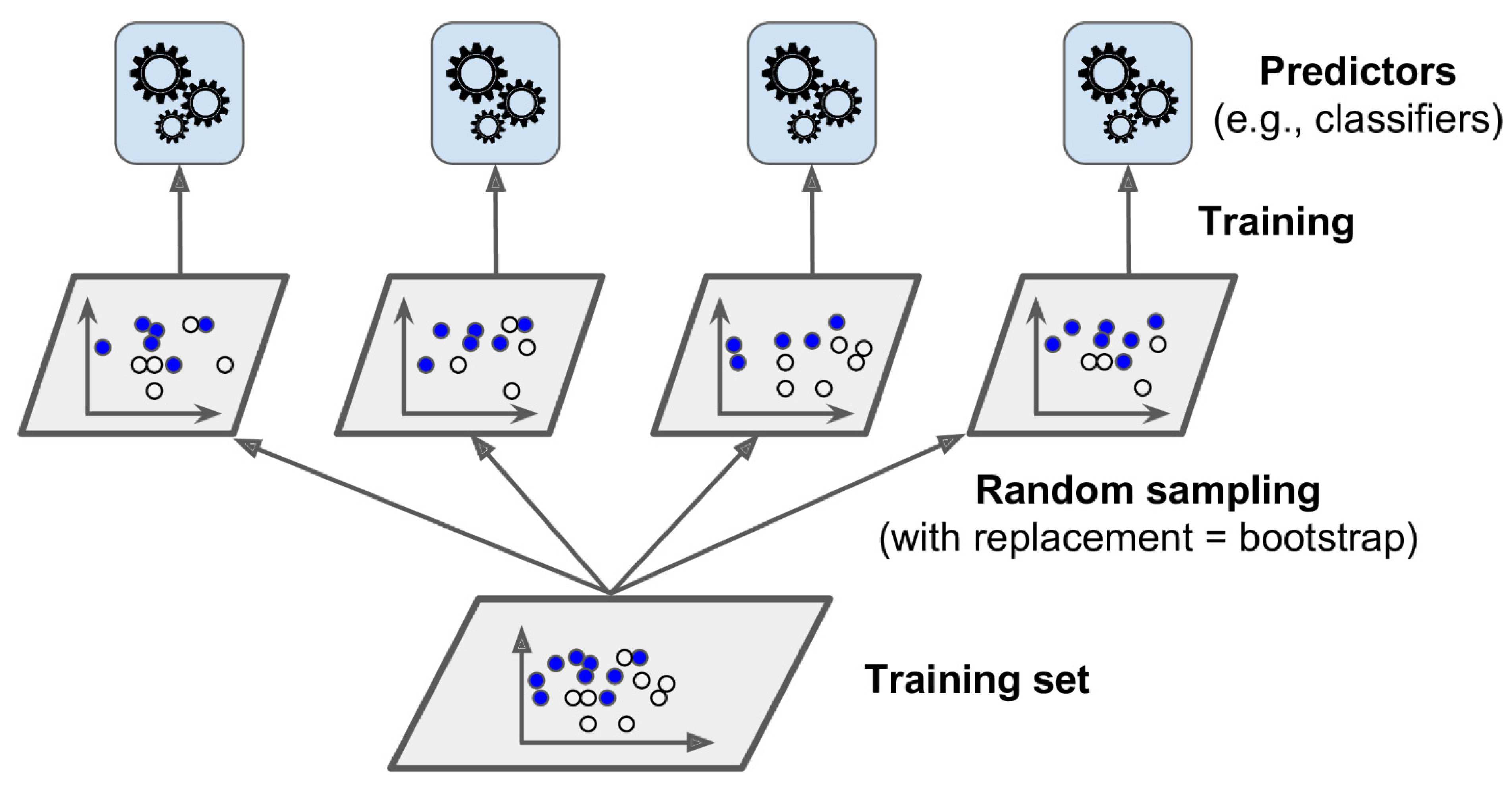
2.2. Bagging
2.3. Random Forest Regressor
3. Materials
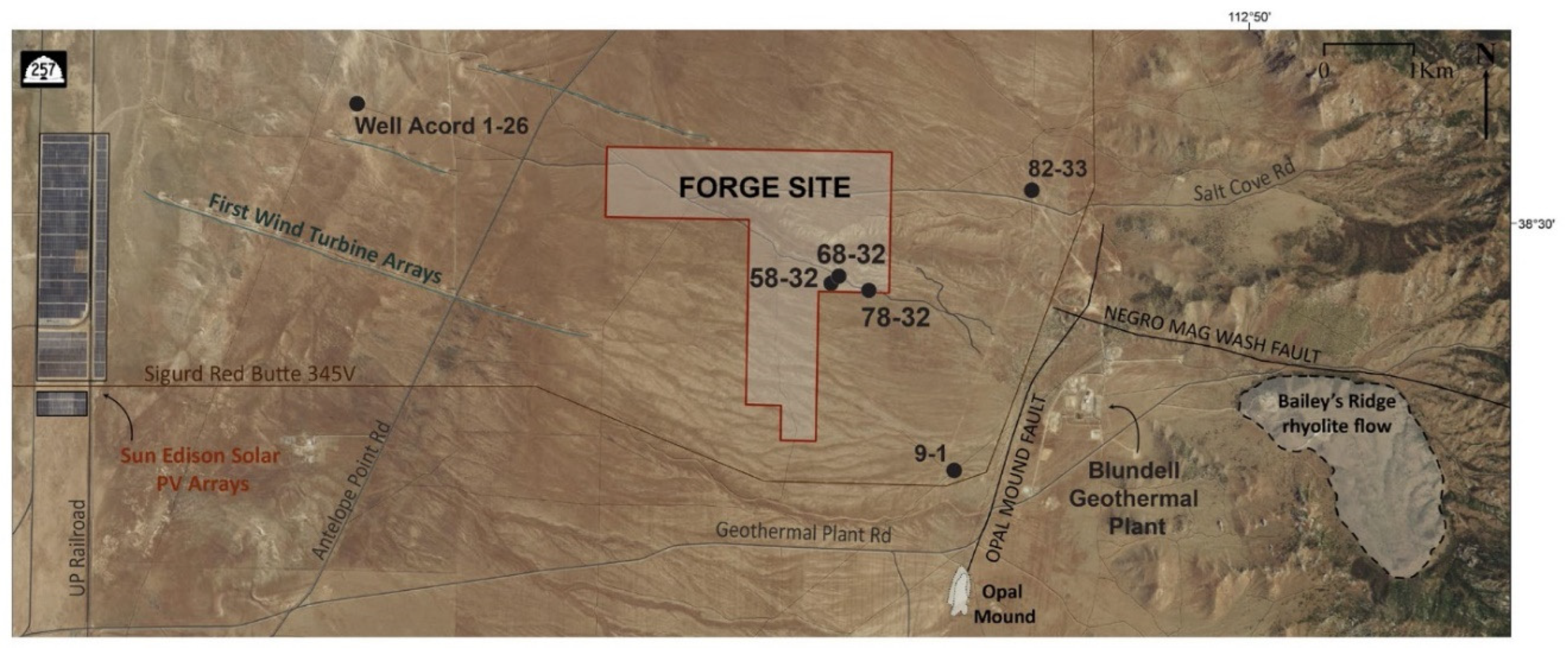
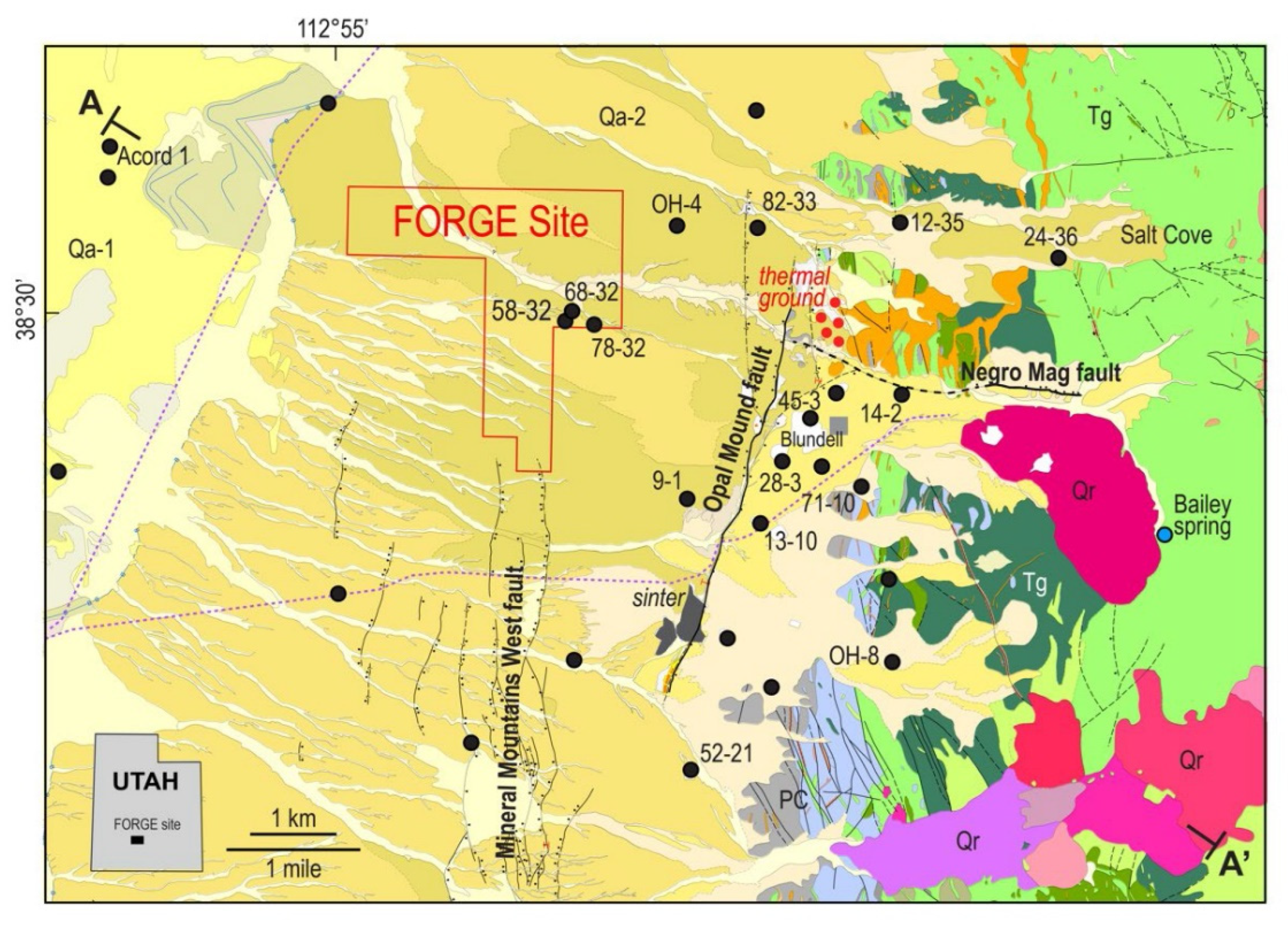
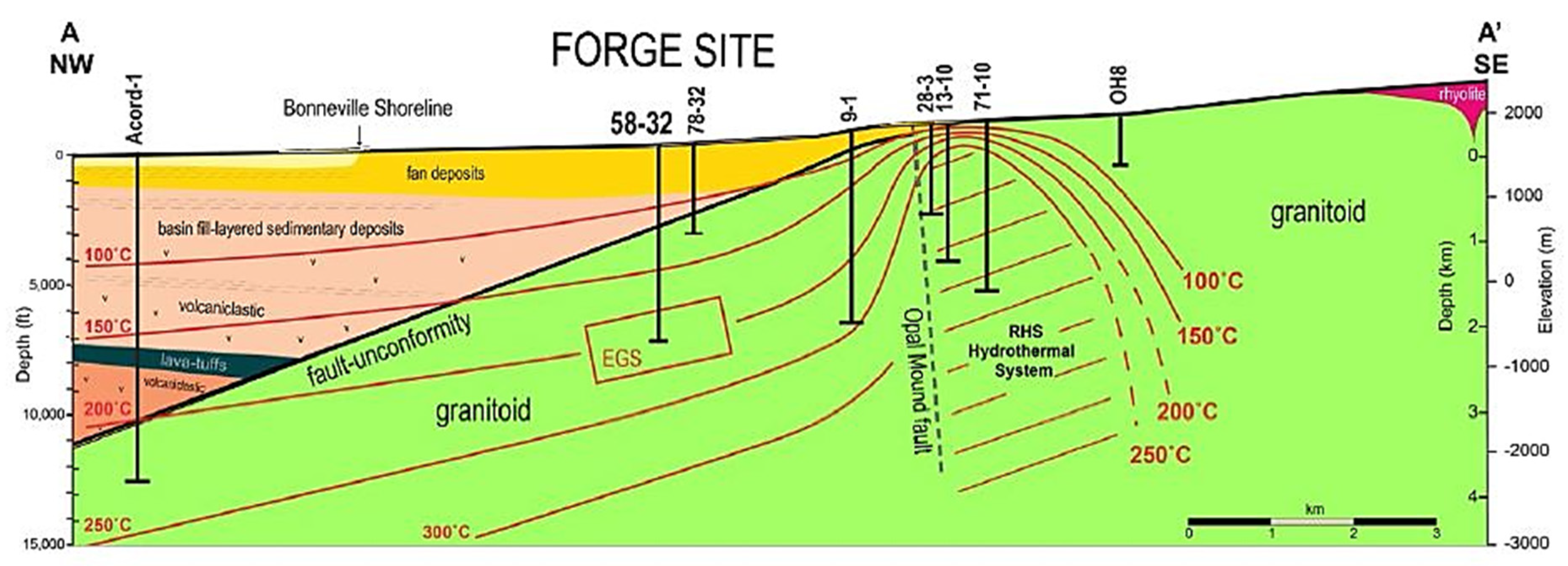
3.1. Study Area
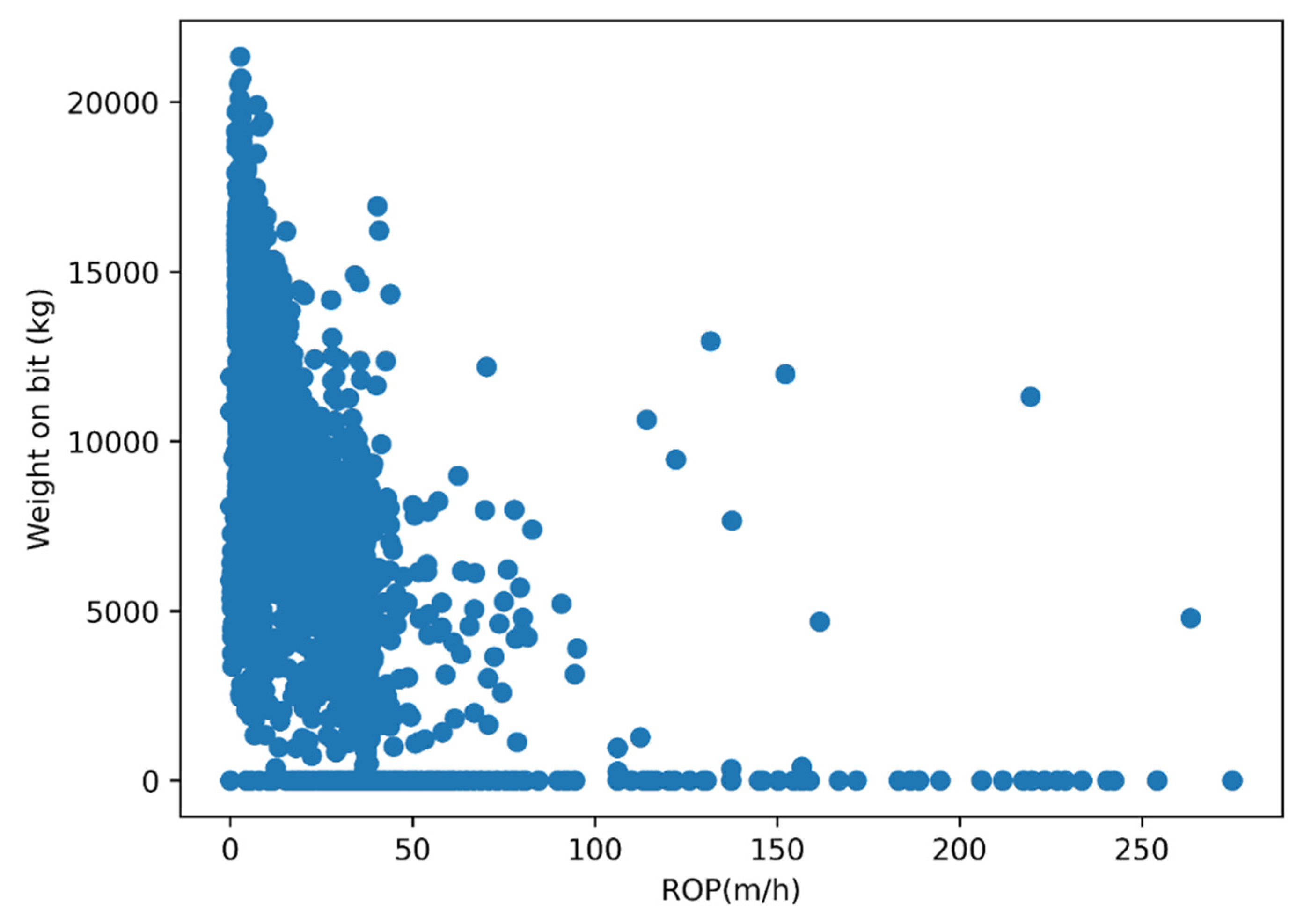
3.2. Drilling Dataset
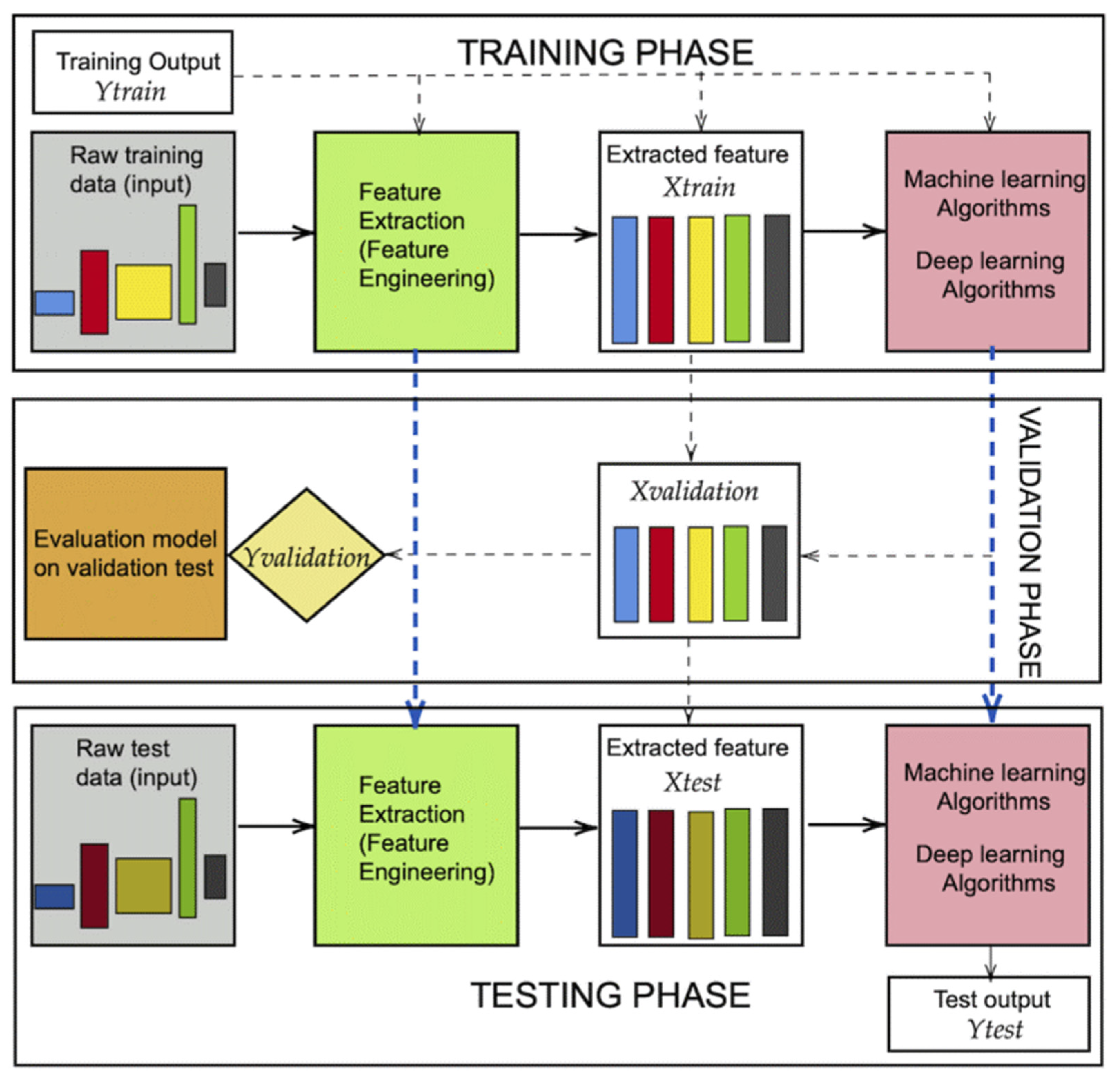
4. Methods
4.1. Data Preprocessing
4.1.1. Feature Selection Based on Domain Knowledge
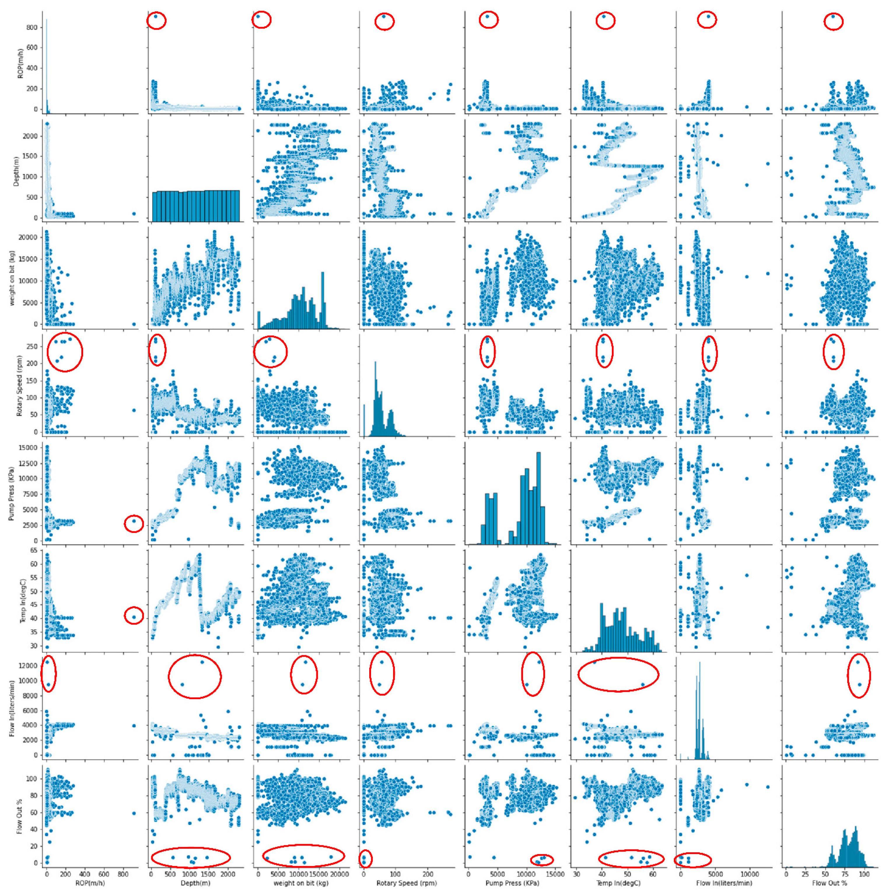
4.1.2. Correlation Measurement
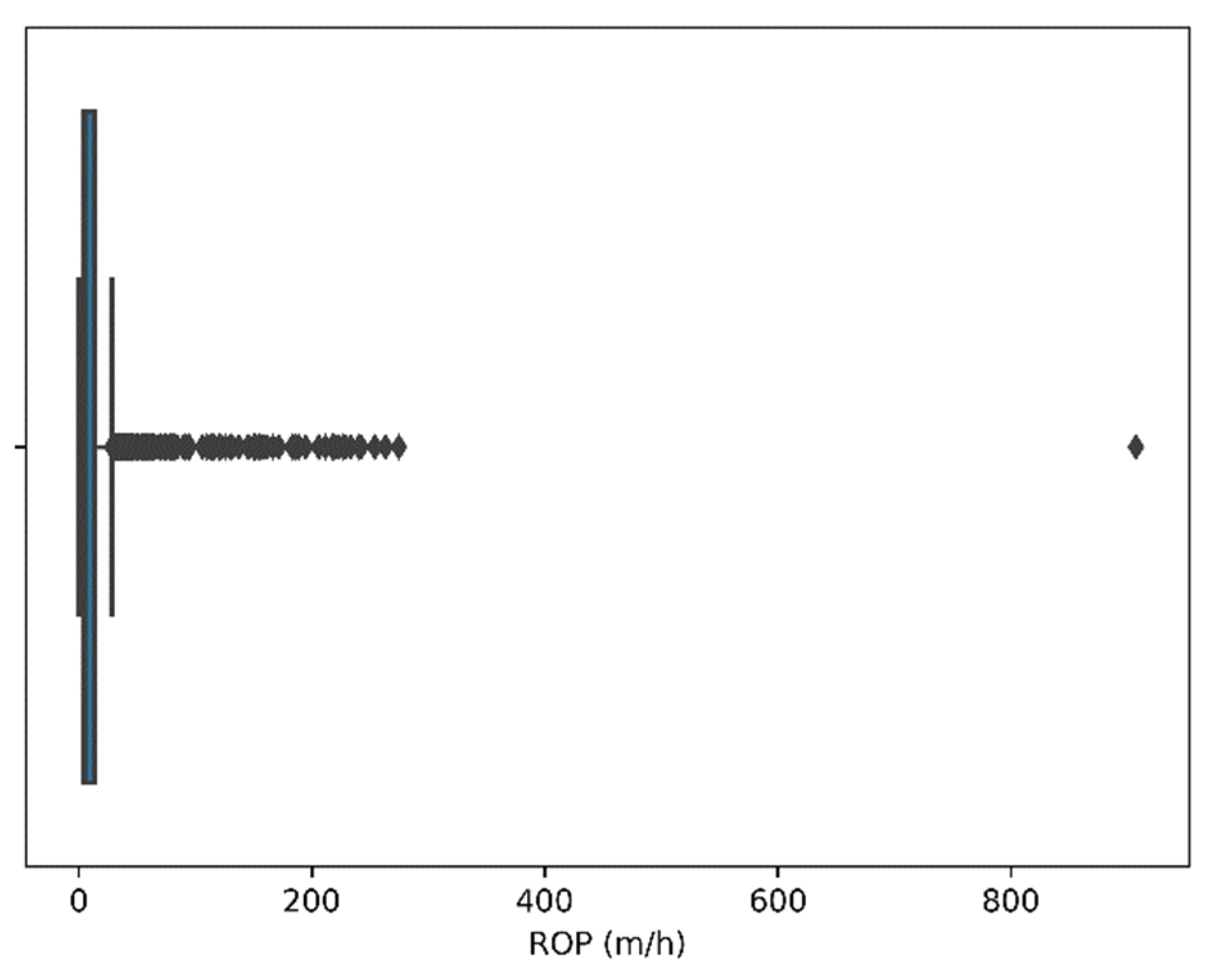
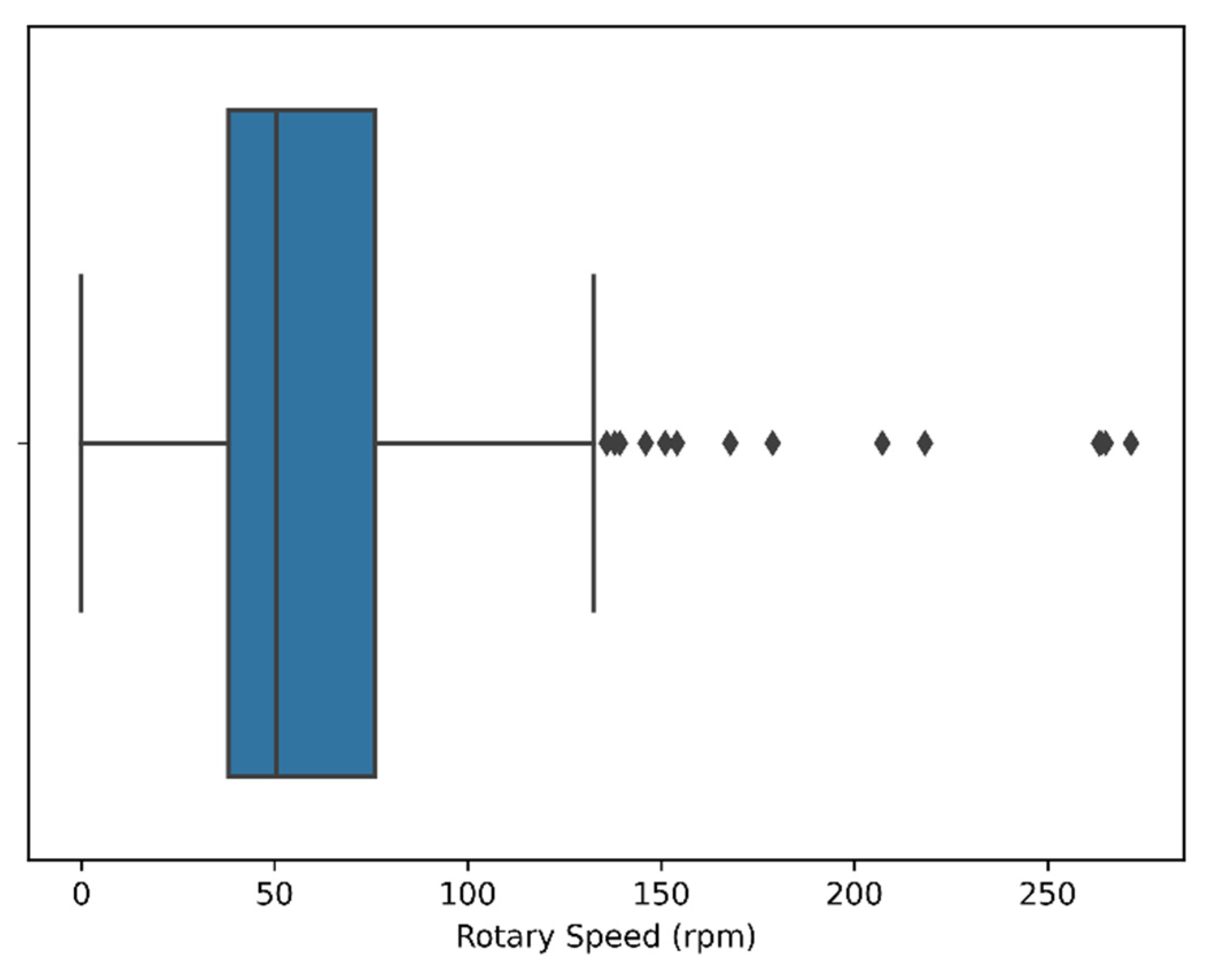
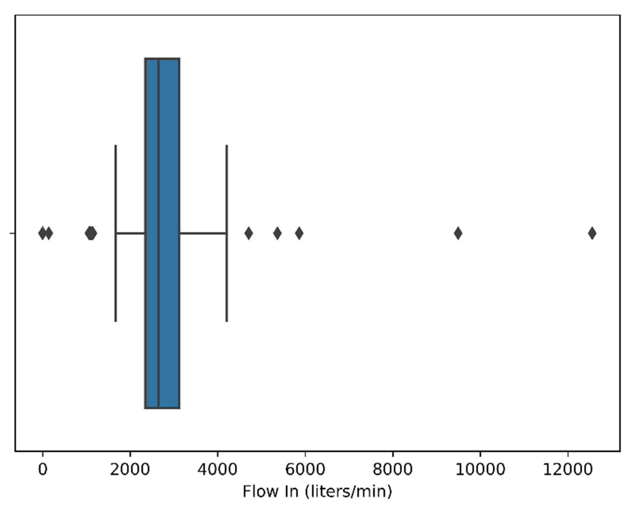
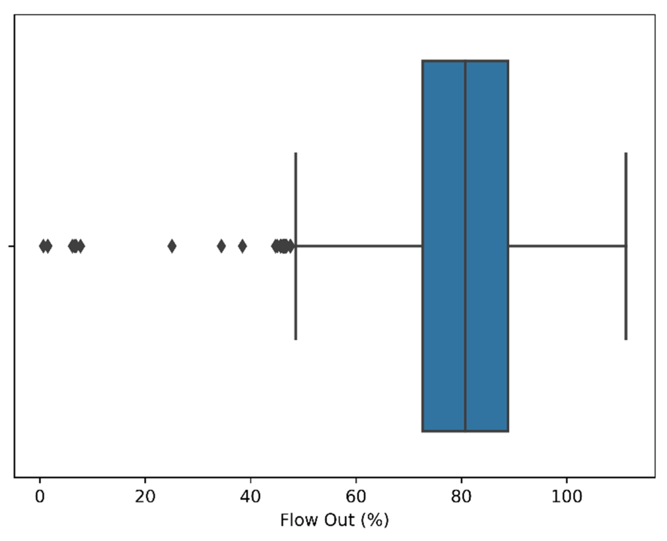
4.1.3. Outlier Removal
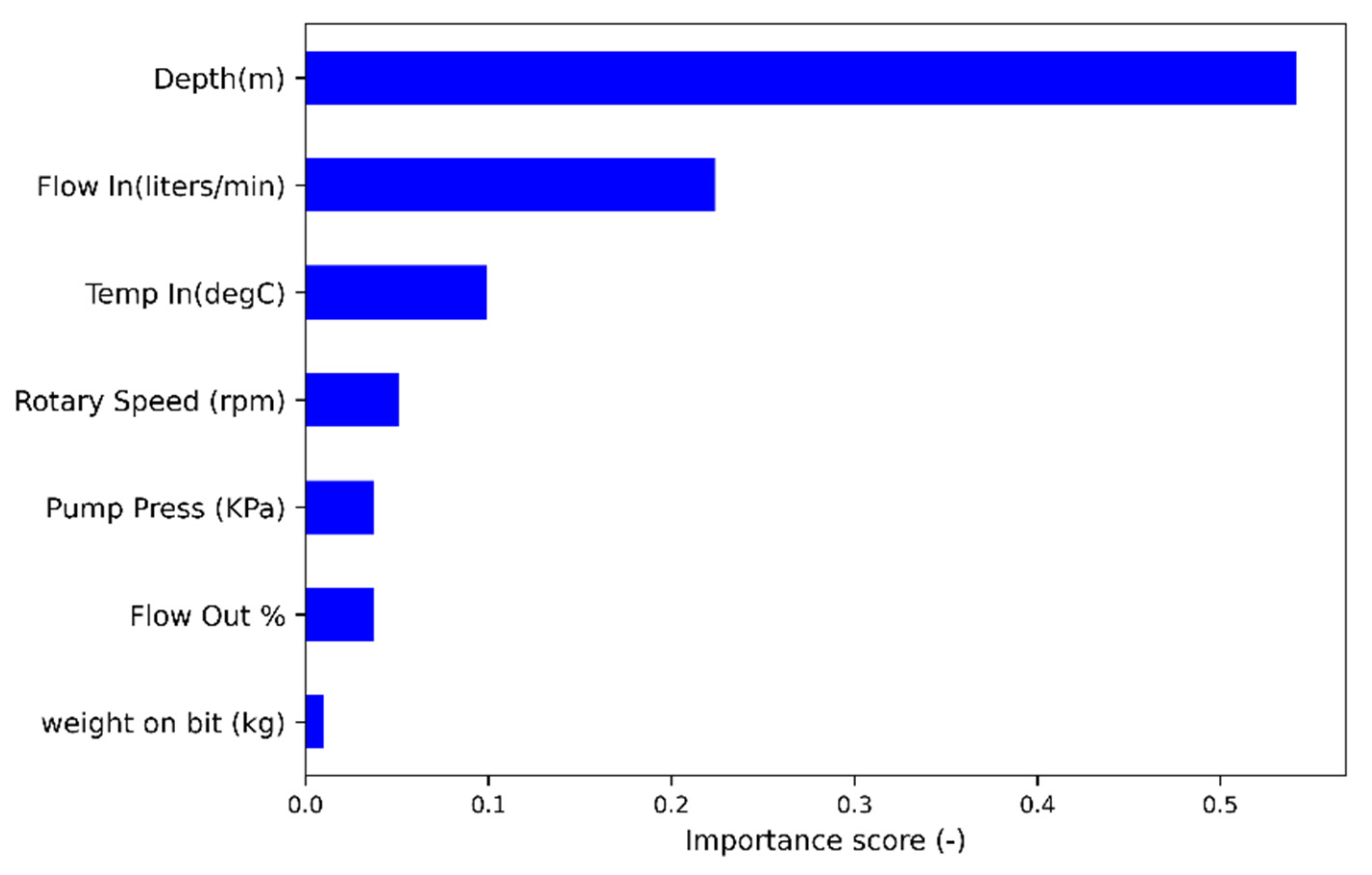
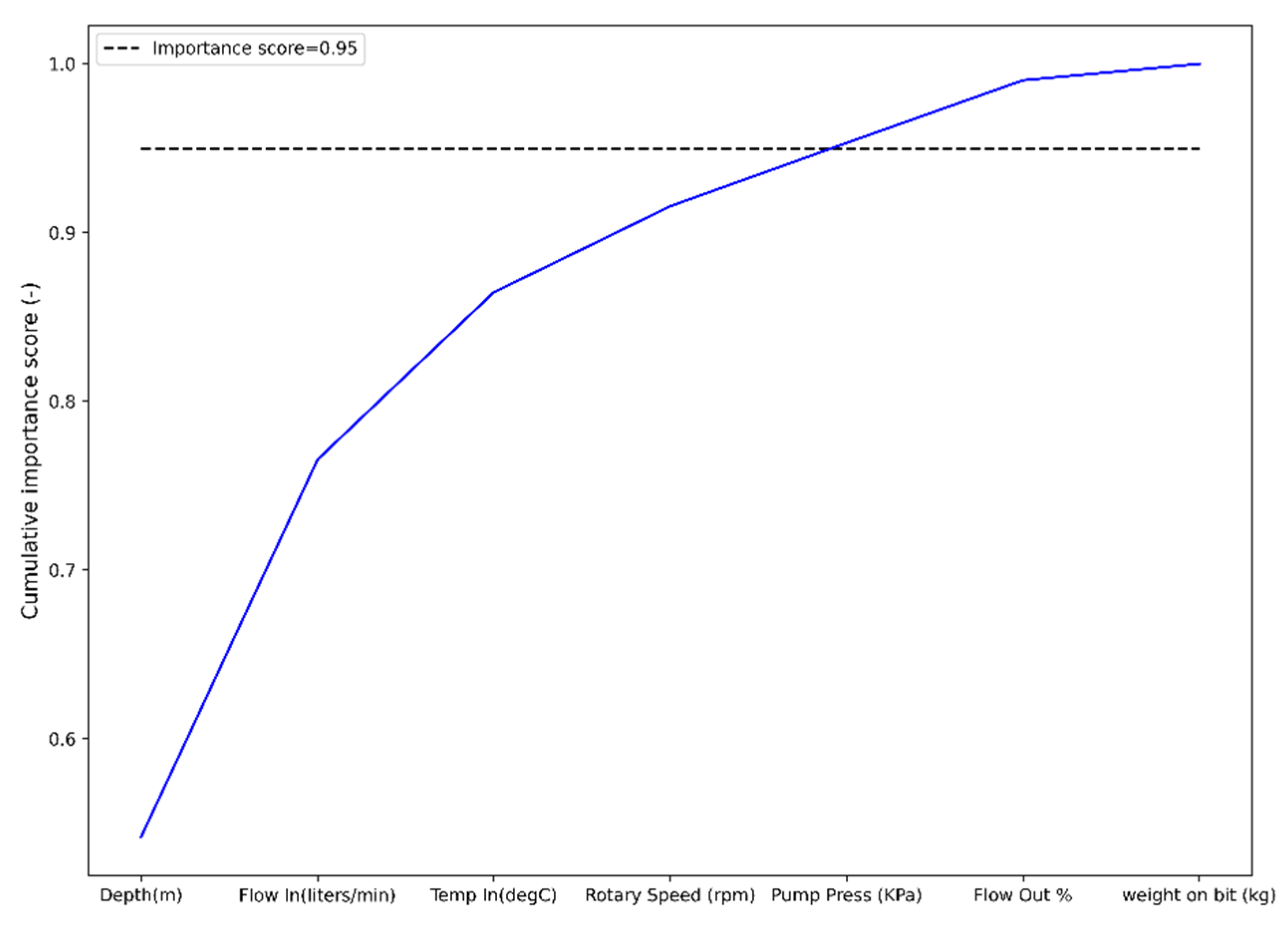
4.1.4. Tree Based Feature Selection
4.1.5. Data Scaling
4.2. Accuracy Assessment of Regression Models
4.3. Model Selection
5. Results
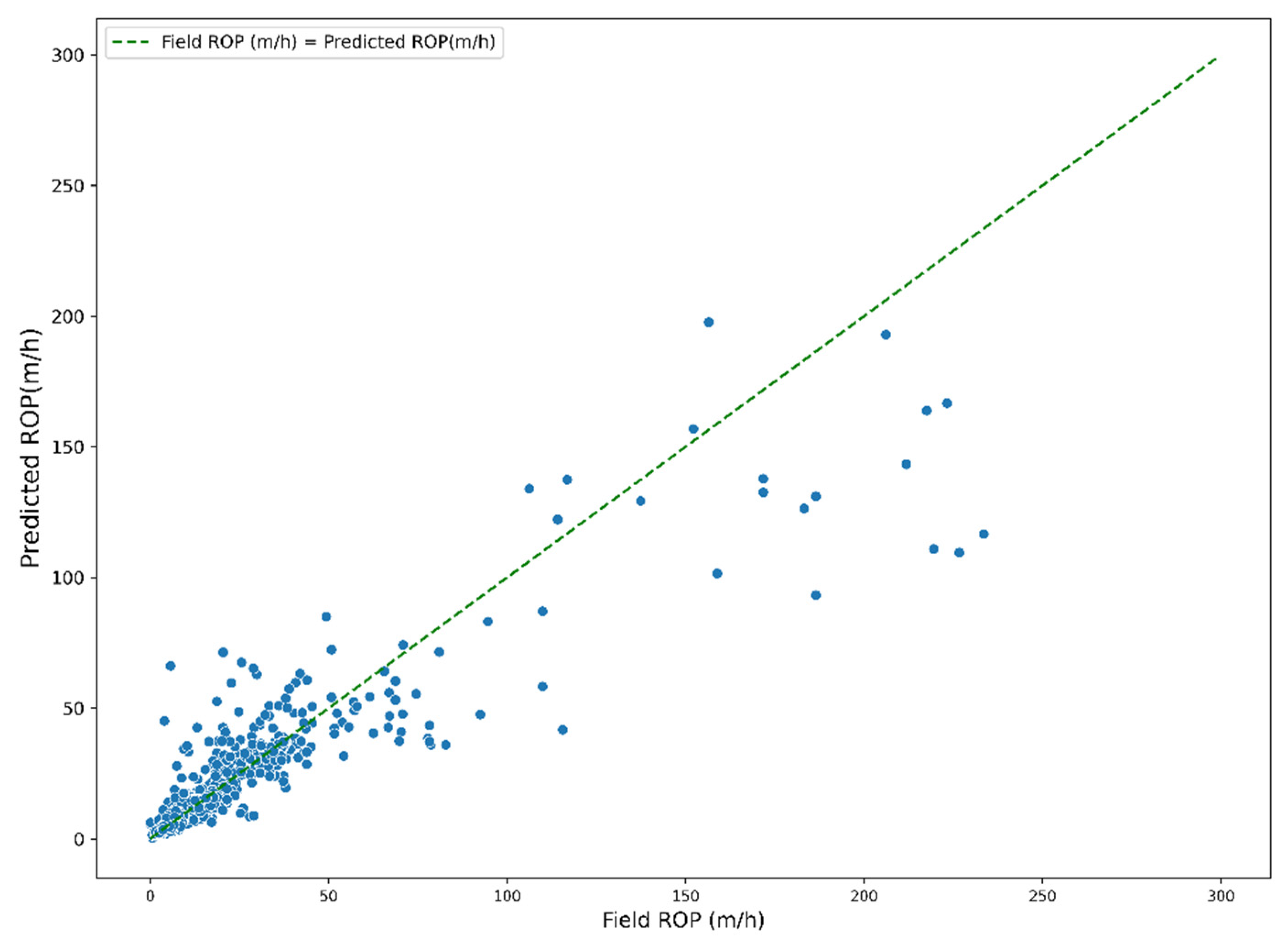
5.1. Training and Cross-Validation of Random Forest Regressor
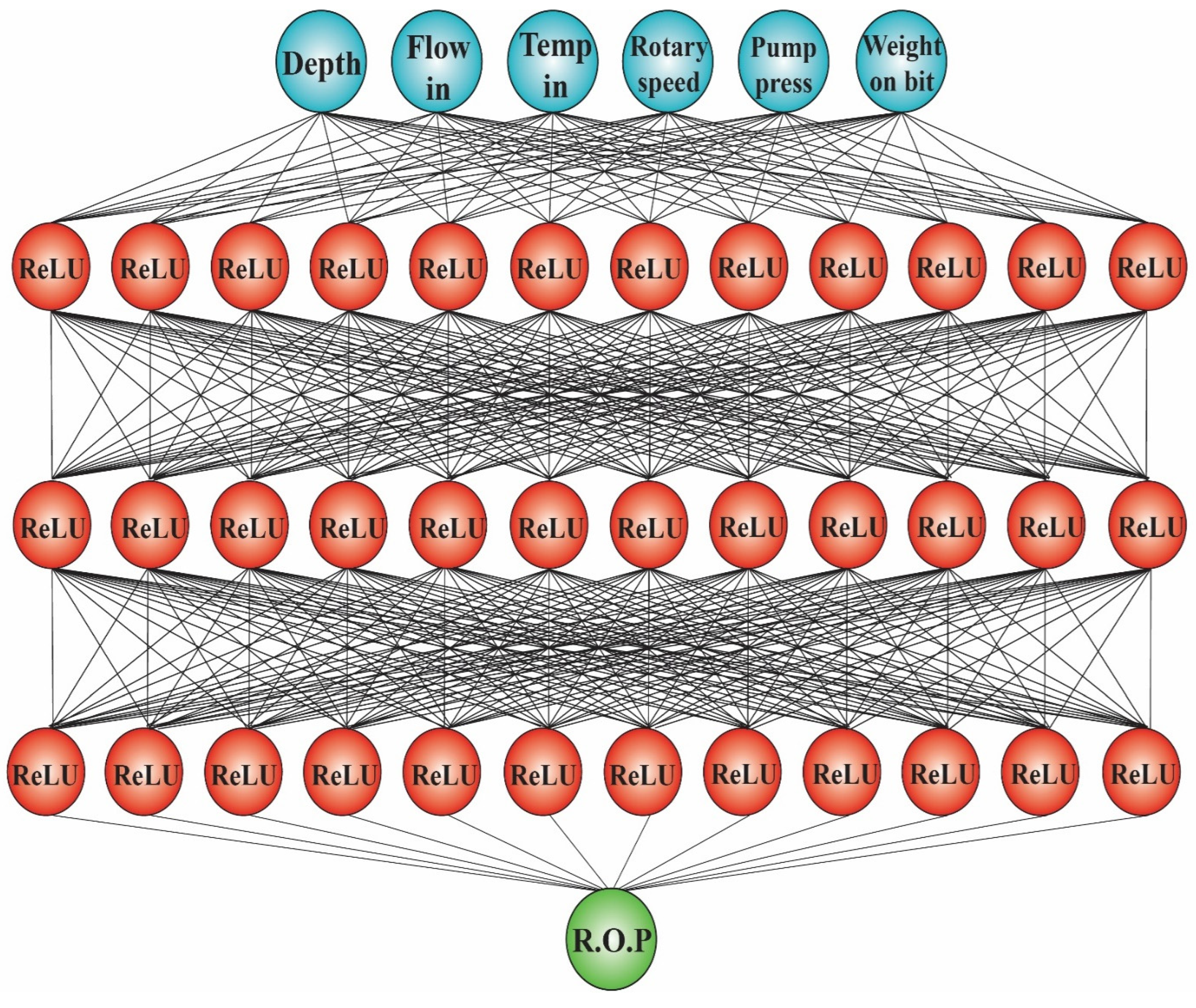
5.2. Training and Cross-Validation Artificial Neural Network
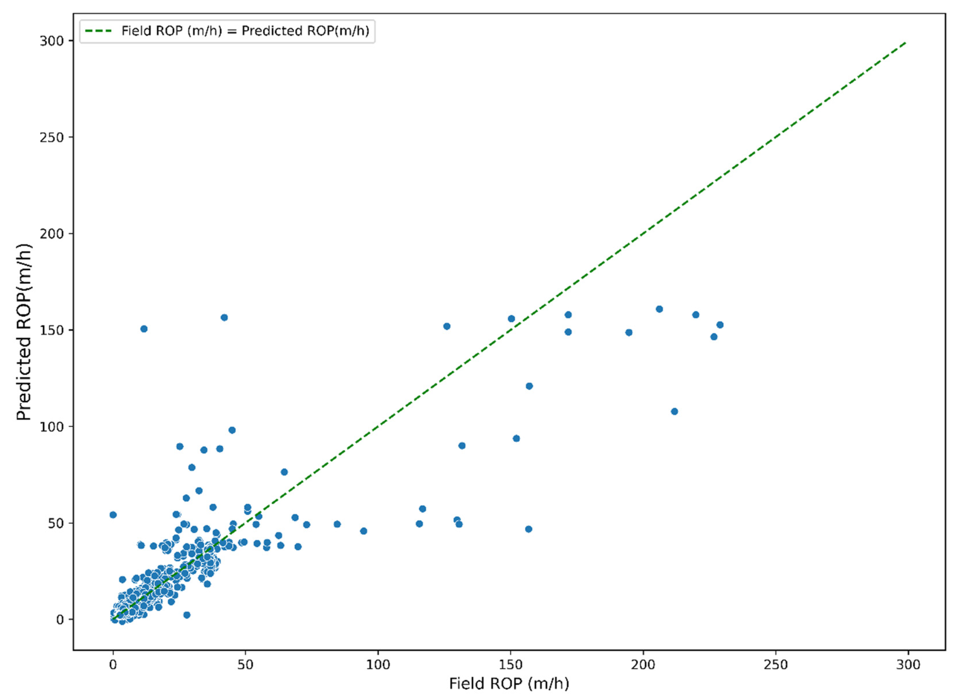
5.3. Model Comparison
6. Discussion
7. Conclusions
Author Contributions
Funding
Institutional Review Board Statement
Informed Consent Statement
Data Availability Statement
Acknowledgments
Conflicts of Interest
References
- Capuano, L.E. Geothermal well drilling. In Geothermal Power Generation; Elsevier: Amsterdam, The Netherlands, 2016; pp. 107–139. [Google Scholar] [CrossRef]
- Thorhallsson, S.; Sveinbjornsson, B.M. Geothermal drilling cost and drilling effectiveness. In Proceedings of the Short Course on Geothermal Development and Geothermal Wells, Santa Tecla, El Salvador, 11–17 March 2012. [Google Scholar]
- Soares, C.; Gray, K. Real-time predictive capabilities of analytical and machine learning rate of penetration (ROP) models. J. Pet. Sci. Eng. 2018, 172, 934–959. [Google Scholar] [CrossRef]
- Maurer, W.C. The ‘Perfect—Cleaning’ Theory of Rotary Drilling. J. Pet. Technol. 1962, 14, 1270–1274. [Google Scholar] [CrossRef]
- Alawami, M. A real-time indicator for the evaluation of hole cleaning efficiency. In Proceedings of the SSPE/IATMI Asia Pacific Oil & Gas Conference and Exhibition, Bali, Indonesia, 29–31 October 2019. [Google Scholar]
- Bourgoyne, A.T.; Millheim, K.K.; Chenevert, M.E.; Young, F.S. Applied Drilling Engineering; Society of Petroleum Engineers: Richardson, TX, USA, 1986; Volume 2. [Google Scholar]
- Dupriest, F.E.; Koederitz, W.L. Maximizing Drill Rates with Real-Time Surveillance of Mechanical Specific Energy. In Proceedings of the SPE/IADC Drilling Conference, Amsterdam, The Netherlands, 23–25 February 2005. [Google Scholar] [CrossRef]
- Young, F.S., Jr. Dynamic Filtration During Microbit Drilling. J. Pet. Technol. 1967, 19, 1209–1224. [Google Scholar] [CrossRef]
- Bourgoyne, A.T., Jr.; Young, F.S., Jr. A Multiple Regression Approach to Optimal Drilling and Abnormal Pressure Detection. Soc. Pet. Eng. J. 1974, 14, 371–384. [Google Scholar] [CrossRef]
- Shi, X.; Meng, Y.; Li, G.; Li, J.; Tao, Z.; Wei, S. Confined compressive strength model of rock for drilling optimization. Petroleum 2015, 1, 40–45. [Google Scholar] [CrossRef]
- Brenjkar, E.; Delijani, E.B. Computational prediction of the drilling rate of penetration (ROP): A comparison of various machine learning approaches and traditional models. J. Pet. Sci. Eng. 2022, 210, 110033. [Google Scholar] [CrossRef]
- Alsaihati, A.; Elkatatny, S.; Gamal, H. Rate of penetration prediction while drilling vertical complex lithology using an ensemble learning model. J. Pet. Sci. Eng. 2021, 208, 109335. [Google Scholar] [CrossRef]
- Atashnezhad, A.; Akhtarmanesh, S.; Hareland, G.; Al Dushaishi, M. Developing a Drilling Optimization System for Improved Overall Rate of Penetration in Geothermal Wells. In Proceedings of the 55th U.S. Rock Mechanics/Geomechanics Symposium, Virtual, 18–25 June 2021. [Google Scholar]
- Mitchell, T.M. Machine learning and data mining. Commun. ACM 1999, 42, 30–36. [Google Scholar] [CrossRef]
- Breiman, L.; Friedman, J.H.; Olshen, R.A.; Stone, C.J. Classification and Regression Trees, 1st ed.; Routledge: London, UK, 2017. [Google Scholar] [CrossRef]
- Hastie, T.; Tibshirani, R.; Friedman, J.H. The Elements of Statistical Learning—Data Mining, Inference, and Prediction, 2nd ed.; Springer: New York, NY, USA, 2001. [Google Scholar]
- James, G.; Witten, D.; Hastie, T.; Tibshirani, R. An Introduction to Statistical Learning; Springer: New York, NY, USA, 2013; Volume 103. [Google Scholar] [CrossRef]
- Friedman, J.H. Greedy Function Approximation: A Gradient Boosting Machine. Ann. Stat. 2001, 29, 1189–1232. [Google Scholar] [CrossRef]
- Breiman, L. Bagging predictors. Mach. Learn. 1996, 24, 123–140. [Google Scholar] [CrossRef]
- Breiman, L. Random Forests. Mach. Learn. 2001, 45, 5–32. [Google Scholar] [CrossRef]
- Géron, A. Hands-on Machine Learning with Scikit-Learn and Tensorflow: Concepts; O’Reilly Media, Inc.: Sebastopol, CA, USA, 2017. [Google Scholar]
- Moore, J.; McLennan, J.; Pankow, K.; Simmons, S.; Podgorney, R.; Wannamaker, P.; Xing, P. The Utah Frontier Observatory for Research in Geothermal Energy (FORGE): A Laboratory for Characterizing, Creating and Sustaining Enhanced Geothermal Systems. In Proceedings of the 45th Workshop on Geothermal Reservoir Engineering, Stanford, CA, USA, 10–12 February 2020; p. 10. [Google Scholar]
- Frontier Observatory for Research in Geothermal Energy (FORGE). Phase 2B Tropical Report; University of Utah: Salt Lake City, UT, USA, 2018. [Google Scholar]
- Allis, R.; Moore, J.; Davatzes, N.; Gwynn, M.; Hardwick, C.; Kirby, S.; Simmons, S. EGS Concept Testing and Development at the Milford, Utah FORGE Site. In Proceedings of the 41st Workshop on Geothermal Reservoir Engineering, Stanford, CA, USA, 22–24 February 2016; p. 13. [Google Scholar]
- Simmons, S.F.; Kirby, S.; Bartley, J.; Allis, R.; Kleber, E.; Knudsen, T.; Moore, J. Update on the Geoscientific Understanding of the Utah FORGE Site. In Proceedings of the 44th Workshop on Geothermal Reservoir Engineering, Stanford, CA, USA, 11–13 February 2019; p. 10. [Google Scholar]
- Kirby, S.M.; Knudsen, T.; Kleber, E.; Hiscock, A. Geologic Setting of the Utah FORGE Site, Based on New and Revised Geologic Mapping. Trans. Geotherm. Resour. Counc. 2018, 42, 1097–1114. [Google Scholar]
- Nielson, D.L.; Evans, S.H., Jr.; Sibbett, B.S. Magmatic, structural, and hydrothermal evolution of the Mineral Mountains intrusive complex, Utah. GSA Bull. 1986, 97, 765–777. [Google Scholar] [CrossRef]
- Podgorney, R. Utah FORGE: Drilling Data for Student Competition; Idaho National Laboratory: Idaho Falls, ID, USA, 2018. [Google Scholar] [CrossRef]
- Kuhn, M.; Johnson, K. Applied Predictive Modeling; Springer: New York, NY, USA, 2013. [Google Scholar] [CrossRef]
- Majdoub, A. Development of a Machine Learning Model Based on Feature Selection to Predict Volve Production Rate. DiscoverVolve. 2020. Available online: https://www.discovervolve.com/2021/02/23/development-of-a-machine-learning-model-based-on-feature-selection-to-predict-volve-production-rate/ (accessed on 1 May 2022).
- Box, G.E.P.; Tidwell, P.W. Transformation of the Independent Variables. Technometrics 1962, 4, 531–550. [Google Scholar] [CrossRef]
- Geladi, P.; Manley, M.; Lestander, T. Scatter plotting in multivariate data analysis. J. Chemom. 2003, 17, 503–511. [Google Scholar] [CrossRef]
- Guyon, I.; Elisseeff, A. An Introduction to Variable and Feature Selection. J. Mach. Learn. Res. 2003, 3, 1157–1182. [Google Scholar]
- Zhou, Z.; Hooker, G. Unbiased Measurement of Feature Importance in Tree-Based Methods. ACM Trans. Knowl. Discov. Data 2021, 15, 1–21. [Google Scholar] [CrossRef]
- Patro, S.G.K.; Sahu, K.K. Normalization: A Preprocessing Stage. arXiv 2015, arXiv:150306462. [Google Scholar] [CrossRef]
- Wackerly, D.D.; Mendenhall, W.; Scheaffer, R.L. Mathematical Statistics with Applications, 7th ed.; International ed.; Thomson Higher Education: Belmont, CA, USA, 2008. [Google Scholar]
- Barten, A.P. The coefficient of determination for regression without a constant term. In The Practice of Econometrics; Heijmans, R., Neudecker, H., Eds.; Springer: Dordrecht, The Netherlands, 1987; Volume 15, pp. 181–189. [Google Scholar] [CrossRef]
- James, G.M. Variance and Bias for General Loss Functions. Mach. Learn. 2003, 51, 115–135. [Google Scholar] [CrossRef]
- Browne, M.W. Cross-Validation Methods. J. Math. Psychol. 2000, 44, 108–132. [Google Scholar] [CrossRef]
- Xu, Y.; Goodacre, R. On Splitting Training and Validation Set: A Comparative Study of Cross-Validation, Bootstrap and Systematic Sampling for Estimating the Generalization Performance of Supervised Learning. J. Anal. Test. 2018, 2, 249–262. [Google Scholar] [CrossRef] [PubMed]
- Bengio, Y.; Grandvalet, Y. No Unbiased Estimator of the Variance of K-Fold Cross-Validation. J. Mach. Learn. Res. 2004, 5, 1089–1105. [Google Scholar]
- Goodfellow, I.; Bengio, Y.; Courville, A. Deep Learning; The MIT Press: Cambridge, MA, USA, 2016. [Google Scholar]
- Nwankpa, C.; Ijomah, W.; Gachagan, A.; Marshall, S. Activation Functions: Comparison of trends in Practice and Research for Deep Learning. arXiv 2018, arXiv:181103378. [Google Scholar]
- Nair, V.; Hinton, G.E. Rectified Linear Units Improve Restricted Boltzmann Machines. In Proceedings of the 27th International Conference on Machine Learning, Haifa, Israel, 21–24 June 2010; p. 8. [Google Scholar]


| Count | Mean | std | Min | 25% | 50% | 75% | Max | |
|---|---|---|---|---|---|---|---|---|
| Depth (m) | 7311 | 1168.864 | 654.5272 | 25.96 | 600.545 | 1173.99 | 1734.71 | 2296.94 |
| ROP (m/h) | 7311 | 12.80416 | 23.13962 | 0 | 3.47 | 5.48 | 13.5 | 907.62 |
| Weight on Bit (kg) | 7311 | 10,483.76 | 4135.825 | 0 | 8303.85 | 10,807.26 | 13,460.32 | 21,337.87 |
| Temp Out (°C) | 7311 | 52.2553 | 6.811023 | 28.93 | 46.74 | 51.59 | 58.05 | 66.5 |
| Temp In (°C) | 7311 | 47.95309 | 6.629486 | 29.44 | 42.695 | 47.34 | 52.7 | 63.51 |
| Pit Total (m3) | 7311 | 37.6687 | 2.9034 | 27.17 | 35.7 | 37.86 | 39.68 | 44.5 |
| Pump Press (KPa) | 7311 | 8733.445 | 3382.374 | 137.49 | 4589.24 | 9877.5 | 11,512.44 | 1,5171.96 |
| Hook Load (kg) | 7311 | 36,864.21 | 12019.88 | 12,367.35 | 24,816.33 | 36,344.67 | 47,904.76 | 67,541.95 |
| Surface Torque (KPa) | 7311 | 903.1323 | 335.8324 | 0 | 806.715 | 967.44 | 1084.45 | 1887.23 |
| Rotary Speed (rpm) | 7311 | 54.94729 | 25.94765 | 0 | 38.09 | 50.38 | 75.965 | 271.58 |
| Flow In (liters/min) | 7311 | 2711.315 | 536.7113 | 0 | 2347.94 | 2650.58 | 3121.485 | 12,558.14 |
| Flow Out % | 7311 | 79.69283 | 11.9094 | 0.69 | 72.65 | 80.71 | 88.845 | 111.21 |
| WH Pressure (KPa) | 7311 | −246.571 | 1535.307 | −8493.47 | 20.13 | 40.96 | 56.95 | 120.04 |
| H2S Floor | 7311 | −0.02737 | 0.042453 | −0.1 | −0.07 | −0.01 | 0 | 0.78 |
| H2S Cellar | 7311 | 0.004303 | 0.025282 | −0.08 | −0.01 | 0 | 0.02 | 0.07 |
| H2S Pits | 7311 | 0.148833 | 0.11529 | −0.06 | 0.06 | 0.14 | 0.22 | 0.72 |
| Predictors | Pearson Correlation between ROP (m/h) and Predictors |
|---|---|
| Depth (m) | −0.508247 |
| Weight on Bit (kg) | −0.523441 |
| Rotary Speed (rpm) | 0.28907 |
| Pump Press (KPa) | −0.49319 |
| Temp In (degC) | −0.221713 |
| Flow In (liters/min) | 0.481607 |
| Flow Out % | −0.116068 |
| ROP (m/h) | Depth (m) | Weight on Bit (kg) | Rotary Speed (rpm) | Pump Press (KPa) | Temp In (°C) | Flow In (L/min) | |
|---|---|---|---|---|---|---|---|
| count | 7293 | 7293 | 7293 | 7293 | 7293 | 7293 | 7293 |
| mean | 12.56974 | 1170.125 | 10,492.41894 | 54.855718 | 8737.605204 | 47.953857 | 2710.542394 |
| std | 20.19483 | 654.3972 | 4130.250795 | 25.296998 | 3378.177407 | 6.626395 | 511.248043 |
| min | 0 | 25.96 | 0 | 0 | 137.49 | 29.44 | 0 |
| 25% | 3.47 | 601.94 | 8308.39 | 38.12 | 4593.17 | 42.72 | 2347.94 |
| 50% | 5.47 | 1176.13 | 10,807.26 | 50.38 | 9877.5 | 47.34 | 2650.58 |
| 75% | 13.46 | 1736.1 | 13460.32 | 75.95 | 11,510.1 | 52.7 | 3120.96 |
| max | 274.75 | 2296.94 | 21,337.87 | 178.86 | 15,171.96 | 63.51 | 5864.13 |
Publisher’s Note: MDPI stays neutral with regard to jurisdictional claims in published maps and institutional affiliations. |
© 2022 by the authors. Licensee MDPI, Basel, Switzerland. This article is an open access article distributed under the terms and conditions of the Creative Commons Attribution (CC BY) license (https://creativecommons.org/licenses/by/4.0/).
Share and Cite
Ben Aoun, M.A.; Madarász, T. Applying Machine Learning to Predict the Rate of Penetration for Geothermal Drilling Located in the Utah FORGE Site. Energies 2022, 15, 4288. https://doi.org/10.3390/en15124288
Ben Aoun MA, Madarász T. Applying Machine Learning to Predict the Rate of Penetration for Geothermal Drilling Located in the Utah FORGE Site. Energies. 2022; 15(12):4288. https://doi.org/10.3390/en15124288
Chicago/Turabian StyleBen Aoun, Mohamed Arbi, and Tamás Madarász. 2022. "Applying Machine Learning to Predict the Rate of Penetration for Geothermal Drilling Located in the Utah FORGE Site" Energies 15, no. 12: 4288. https://doi.org/10.3390/en15124288
APA StyleBen Aoun, M. A., & Madarász, T. (2022). Applying Machine Learning to Predict the Rate of Penetration for Geothermal Drilling Located in the Utah FORGE Site. Energies, 15(12), 4288. https://doi.org/10.3390/en15124288