Abstract
The energy consumption estimation of a locomotive for a particular route is important for the selection of a locomotive technology, the improvement of the energy management system, the evaluation of the locomotive’s potential energy generation, among others. The methodologies reported in the literature usually assume that the information of the railway track is available; however, in some cases, the track information is incomplete, not available, or the route is still in a planning stage. Therefore, this paper proposes a methodology to estimate the energy consumption and the potential energy generation of a locomotive when the railway track information is not available or incomplete. The methodology begins by extracting the main technical information of the locomotive to be analyzed. Then, the route is traced on Google Earth with steps of 100 m and the obtained information is processed to generate the longitude, latitude, elevation, and distance of the points along the route. From such information, it is possible to generate the slope and curvature profiles, while the speed profile can be obtained from the track operator or the regulations of a specific country. With that information, it is possible to estimate the equivalent power of the locomotive at each point of the route to finally calculate the consumed energy. The proposed methodology is validated with two case studies. The first one compares the results with a methodology available in the literature for the same route and locomotive, while the second case shows the applicability of the proposed methodology for a route without information.
1. Introduction
Worldwide railway systems have promoted technological, social, economic, and industrial progress since the age of steam propulsion [1], due to the significant reduction in travel times and increment of the transported load capacity. Locomotives are the key elements in a railway system; therefore, the selection of a locomotive for a particular railway line, or the replacement of an obsolete locomotive, requires the estimation of the energy consumption considering the track geometry and the main characteristics of the particular locomotive [2,3]. Such energy consumption estimation can be used to compare different locomotives for a specific application, estimate the emissions of greenhouse gases, identify the technology that best suits a particular railway track, and plan new railway routes [4].
Although it is a relevant research focus, few works in the state of the art report a detailed analysis to perform the energy consumption estimation of a locomotive. These works can be divided into two groups, the first one corresponds to the methods based on historical data, resulting from gathering the information of trajectories traveled with operating trains; while the second group corresponds to the methods based on information from railway infrastructure and locomotives, which relate the information to obtain an approximation of the consumption.
Regarding the first group, it is worth mentioning that few countries have a reliable database based on measurements of the condition of their railways and locomotives, which can be used to design a road map for the upgrading of their railway infrastructure [5]. This represents a problem when calculating the energy consumption of a railway system since, for historical-data-based methodologies, such as regressions using neural networks or fuzzy logic [6], it would not be possible to have a reliable database to feed the mathematical models. A particular case of historical-data-based methodologies is China, which estimates its energy consumption on trajectories based on data collected from different railway companies [7], facilitating statistical regressions with minimal errors. In addition to energy consumption calculation methodologies, other research areas, with an environmental impact focus, also require information about the railway and the trains when designing their calculation methodologies in terms of environmental pollution [8]. Such is the case of [9], where the authors described an effort of more than eight years for the collection of data for operating locomotives in the Brazilian railway system, exposing the problems of acquiring the necessary information to estimate their environmental indicators.
Methodologies based on historical data denote previously known data about the analyzed route. Such information is retrieved from databases built by the railway systems themselves, which have a technological infrastructure to gather information on each trajectory such as track condition, speeds, accelerations, times, among others. For example, in [10], the main contribution was to optimize the energy consumption for a mountainous trajectory by implementing an energy management system with batteries. Among the several important results reported, the author mentioned that the railway data were taken from a database provided by a railway company for the trajectory between Zagreb and Split, Croatia. Due to the information provided by the railway company, years later, the paper reported in [11] described an energy analysis for the Lika-Senj region with the same purpose of reducing energy consumption. Both works focused on simulating and estimating the electrical performance of the batteries through a MATLAB/Simulink model, which did not describe the design or the information required to estimate the energy parameters. In addition, the reported results were not compared with field experiments, since their main contribution lay in adding batteries to locomotives that did not have such technology yet.
Moreover, in the work presented in [12], the authors proposed to estimate the energy consumption and used it to calculate economic indicators, to reflect the impact generated from a strategy to reduce energy consumption and, consequently, to reduce the economic impact. This extensive work proposed a neural network to manage a DC microgrid of motors, batteries, and other electrical loads. The case study and its results were based on railway information published by [13], in which the collaboration of the French railway network was highlighted. Such information about the railway provided by the company served many other authors as a database to feed the energy consumption models for the proposed locomotives [14]. Additionally, it is important to mention that this work did not include experimental results.
On the other hand, the energy consumption estimation methodologies based on railway track information require detailed data from the railway track and the locomotive for trajectories without historical data of speeds, accelerations, times, etc. For example, to optimize fuel consumption in the locomotives of the Israeli railway system, the work proposed in [15] described an optimization technique that again required railway information. Although in this work they relied on Google Maps to highlight the route and showed an elevation profile of the studied trajectory, it was not explained if this information was obtained by some methodology to extract information from the map or if it was retrieved from some database.
Nevertheless, there are alternatives to calculate this energy consumption, through the characterization of the railway and the locomotive moving along it. To achieve this, it is necessary to perform an analysis using Newton’s second law, which allows us to know the mechanical stresses around the locomotive; thereby, it is possible to estimate the power required to move the train at each point of the trajectory [16]. This methodology requires technical information about the locomotive, such as tractive effort, braking effort, maximum speed, among others. Likewise, it is necessary to know the characteristics of the railway to consider the opposing forces to the movement of the locomotive, such as the slope, curvature radius, and track gauge [17,18,19,20].
Such is the case of the work proposed by [21], which estimated the energy consumption of a locomotive in the Cartagena–Albacete trajectory of the Spanish railway system; to achieve this, the authors gathered information from the locomotive and the technical profile of the track of this path. Although this way of calculating energy consumption requires less information based on experience than the methodologies based on historical data, it still depends on information retrieved from databases, experimental measurements from the railway operators, or from companies in the railway sector that have at least mapped their trajectories. These characteristics restrict the application of this type of methodologies to railway systems that do not have technical information on their tracks.
Based on the state of the art, it is evident at this point how the works reported so far require information provided by the companies managing the railroads along with the locomotives operating on them. Otherwise, if such information is not provided or does not exist, it is not possible to estimate the energy consumption of a locomotive based on the methodologies analyzed in this section since, as previously reported, those methodologies require the trajectory information to obtain their results. It is worth noting that some software tools such as Google Earth [22,23] or GPS Visualizer [24] can be used to trace the railway track and obtain the latitude, longitude, and elevation of multiple points along the track. However, these tools do not provide the curvature, slope, and speed profiles required to implement the energy consumption estimation methodologies based on the railway track information. Other tools, such as the one introduced in [25], estimate the curvature of different roads and use a color scale to classify the curves from “moderate twisty” to “very twisty”. Nevertheless, this tool cannot be used to generate the curvature profile of a railway track.
Hence, this paper proposes a methodology to estimate the power consumption of a locomotive when the railway geometry information is not complete or is not available at all. The methodology requires the main data from the locomotive, which can be obtained from its datasheet or the manufacturer documentation, and the main information about the railway features (elevation profile, curvature profile, and slope profile) is estimated from the latitude, longitude, and elevation of multiple points along the track. Moreover, if the speed profiles are not available, they are generated from the national and international regulations considering the maximum theoretical speed as a restriction. From these data, it is possible to apply Newton’s laws to estimate the net force of the locomotive at each point of the track, which can be combined with the speed and the motor efficiency to determine the mechanical and electrical power. Then, the methodology estimates the time instant for each calculated electrical power to determine the consumed energy and the potential energy generation of the locomotive along the route. Therefore, the main contributions of this paper are: (1) a procedure to estimate the curvature, elevation, and slope profiles of the track when this information is not available or incomplete, (2) a procedure to estimate the maximum speed profile of a train considering the track geometry, and (3) a detailed procedure to estimate the locomotive mechanical and electrical energy consumed by the locomotive during its acceleration as well as the potential energy generated during its braking.
The rest of the paper is organized as follows: Section 2 shows the mechanical model of the locomotive to estimate the net force and power at each point, as well as the energy estimation; Section 3 introduces the proposed methodology focusing on the estimation of the railway track profiles; Section 4 introduces two case studies to validate the proposed methodology, and the conclusions in Section 5 close the paper.
2. Calculation of the Energy Consumption of a Locomotive
To estimate the energy consumption of a locomotive in a given time window, it is necessary to determine the effective force experienced by the locomotive () and its speed (v) at each time instant. From those variables, it is possible to calculate the mechanical power of the locomotive (P) and then integrate such power to determine the mechanical energy consumption (E). In turn, E can be used to estimate the electrical energy required () and the potential energy that can be generated with a regenerative braking system (). The following subsections describe the procedure used in this paper to calculate , P, E, , and .
2.1. Calculation of the Locomotive Effective Force
The first step is to analyze the interacting forces on the locomotive. For this purpose, Newton’s second law is used at each point of a specific trajectory, along with the acceleration of the train and its total known mass. The free-body diagram of the locomotive at a specific position is shown in Figure 1, where the interacting forces are observed.
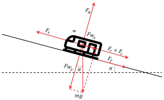
Figure 1.
Free-body diagram of a locomotive.
The application of Newton’s second law to the free-body diagram shown in Figure 1 is introduced in (1), where m represents the train mass, a is the acceleration, is the effort (tractive or braking) of the kth locomotive unit of the train, is the rolling resistance force of kth train element, is the train curve resistance, and is the train gradient force due to the slope of the track. Moreover, k represents the increment of mass due to rotating inertia, which varies from 0 to depending on the type of vehicle and it may take values from to for a complete train. It is important to note that can be positive if the train is ascending, or negative if the train is descending; moreover, u represents the number of locomotives and r the number of train elements (i.e., locomotive, coaches, etc.). The following paragraphs provide a brief description of the forces used in (1).
The rolling resistance force represents the interaction of the train axles with the railway track and the wind effects on the locomotive at a given time. It is represented through Davis’ Equation (2) [26], which is empirically determined considering three main coefficients. The first one is related to the type of locomotive and the type of railway track (), which varies according to the track conditions, associating the resistance generated by the track, the friction between the rail and the wheel, and the effect of the weight on the track. The second and third coefficients ( and ) represent the effect of wind related to aerodynamic force and acceleration changes, which will have more impact at higher speeds.
Moreover, the gravitational force is calculated according to (3) [21], where is the track slope. This expression is related to the weight of the locomotive and the gradient it experiences, which does not exceed in most cases [21,27] due to the power limitations of the locomotives. Additionally, it is worth mentioning that this force may have positive or negative values depending on the inclination of the track.
Another force to be considered in the locomotive motion is the curvature-related force (), which is produced when the wheels of the same axle are coupled and the locomotive is driving through a curve. In this case, there is a sliding effect on the wheel at the inner side of the curve, which generates additional friction that can be calculated with the empirical expression shown in (4) [28], where is a factor attributed to the slippery effect and is the curvature radius in meters.
Additionally, the electrical load in passenger trains, in the case of diesel units, is provided directly by the locomotive, which involves a reduction of traction effort. This effect must be considered in the estimation of the tractive effort vs. the speed profile. In the case of electric units, these loads, so-called hotel loads, are supplied by the overhead lines.
Finally, it is important to mention that the analysis of the forces presented before corresponds to a particular point of the track at a given time instant. Hence, this analysis must be performed point-by-point in a given trajectory to estimate the locomotive power and energy consumption.
2.2. Calculation of Mechanical Power and Electric Energy Consumption
The calculation of the locomotive mechanical power (P) is determined through the product of the speed (v) and the total effort of the locomotives at each point of the specific trajectory, as shown in (6), where can be calculated from (1) as shown in (5), where for a given speed is limited by the forces defined in the tractive and braking efforts profiles of each locomotive. It is worth noting that the total effort of the locomotives may take positive or negative values; hence, can also be negative or positive if the locomotive is generating or consuming energy, respectively [29].
After the estimation of , the total energy consumed by the locomotive at time t to move along the analyzed trajectory is calculated by integrating the positive values of in a time window defined by the times and t, as shown in (7) [21]. It is important to highlight that is the total mechanical energy provided by the locomotive; thus, the calculation of the electric energy consumed by the electric motors of the locomotive can be calculated with (8), where is the efficiency of the locomotive’s motors and their power converters.
Finally, the potential electric energy that can be generated with the locomotive at time t can be estimated as shown in (9), which corresponds to the integral of the negative values of multiplied by two efficiencies and one factor. In (9), is the efficiency of the system that receives the energy generated by motors, and is the availability factor and represents the percentage of the locomotive braking mechanical power (i.e., ) that can be used by the regenerative braking system, which may be between 20% and 30% [30]. For example, in a diesel locomotive with a battery bank, would be defined as , where and are the efficiencies of the power converters and the battery bank. Additionally, the typical efficiencies of the main locomotive technologies are illustrated in Table 1 [31,32].

Table 1.
Power conversion efficiencies of the main locomotive technologies [31,32].
In summary, to estimate , , and , it is necessary to know the main characteristics of the locomotive and the railway track geometry to analyze the forces and determine for each point along the track by using (5). With such information, it is possible to calculate at each analyzed point of the track and to use (7)–(9) to estimate , , and , respectively.
3. Proposed Methodology
The flowchart in Figure 2 summarizes the proposed methodology to estimate the power and energy consumed by a locomotive on a given railway track. The process begins by defining the train to be analyzed to determine its main characteristics: tractive effort vs. speed profile, braking effort vs. speed profile, power conversion efficiency, total mass, rail gauge, Davis’ equation constants (, , and with ), nominal power, and maximum speed. It is worth noting that tractive and braking efforts profiles are usually provided as plots in the locomotives’ datasheets; hence, those plots need to be digitized and interpolated to determine the tractive or braking force for a particular speed value.
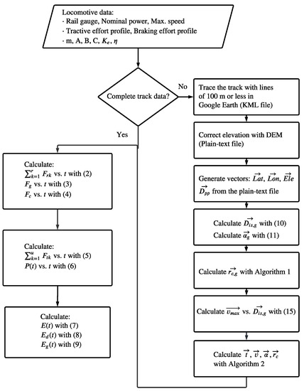
Figure 2.
Flowchart of the proposed methodology.
Then, if the track information is complete, it has to be organized into the following vectors: time (), speed (), slope (), and curvature radius (). Those vectors have n elements, where the ith element of each vector contains the information of the point of the track at time , where . Otherwise, if the railway track information is not available, incomplete, or not reliable, then it is necessary to estimate the vectors described before, by tracing the railway track in a satellite imagery software tool such as Google Earth. The details to estimate , , , and are described in the following subsections.
With complete information from the train and the railway track, it is possible to obtain the values of , , and for each time by evaluating (2), (3), and (4), respectively, with , , and and the other input parameters. Then, the locomotives’ force for each time () is calculated by using (5). Later, combining this information with the train speed given in , it is possible to determine the mechanical power of the locomotives at each time by using (6). Finally, the train power profile is obtained by plotting vs. and the total energy consumed is calculated by integrating the power profile according to (7), while the electrical energy and the potential energy generation can be calculated with (8) and (9), respectively.
The following subsections provide the details to extract the railway track data from satellite imagery as well as the calculation of the determination of the speed ( vs. ), slope ( vs. ), and curvature ( vs. ) time profiles.
3.1. Track Data from Satellite Imagery
The proposed methodology uses Google Earth to obtain the geographical coordinates of the railway track when there is no information or when the information is not complete or reliable. The first step is to trace the railway track using straight lines of 100 m, approximately. Then, the geographical data of each point in the track are exported in a KML file, which is based on the XML language, to provide not only the latitude, longitude, and elevation of each point but other data that can be useful for graphic information system mapping applications.
The elevation data from Google Earth may introduce significant errors in the elevation of each point. Therefore, one option to improve the elevation accuracy is to use the Digital Elevation Model database (DEM), which has a particular database for each region of the planet that best fits the elevation data. Those DEM databases can be accessed through the GPS Visualizer online tool [33], where the user can load a KML file and after a simple process obtain a plain-text file with the position data (i.e., latitude, longitude, and elevation) for each point of the railway track traced on Google Earth. In such a file, the information is organized in rows, where is the number of points used to approximate the track in Google Earth. Moreover, the columns include the point number, latitude (), longitude (), elevation (), and distance between two consecutive points ().
At this point, the plain-text file has the main data required to calculate vs. , vs. , and vs. profiles, which are required for the estimation of the forces acting on the locomotive.
3.2. Calculation of Elevation and Slope vs. Distance Profiles
The generation of the elevation vs. distance and slope profiles calculation begins by generating the vectors and , which contain the elevation and point-to-point distance data, respectively, obtained from the plain-text file described in Section 3.1. From it is simple to calculate a vector with the distance of each point in the track () from the origin by applying (10), where m.
The elevation vs. distance profile can be directly generated by plotting vs. , while the vector with the slopes along the track is calculated from the and vectors. The slope is calculated by assuming a straight line between two consecutive points regarding the elevation; therefore, the slopes are saved in a vector named where the last element is 0o and the rest of the elements are calculated as shown in (11). Then, the slope profile can be generated by plotting vs. .
3.3. Algorithm to Estimate the Curvature Radii vs. Distance Profile
The curvature estimation begins by generating the vectors and from the plain-text file described in Section 3.1. Those vectors have elements that correspond to the points traced along the railway track. Then, the curvature in the point is estimated by analyzing the coordinates of three consecutive points (i, , and with ) of and . Those points form a triangle, as shown in Figure 3; hence, there are triangles along the track. Next, it is necessary to calculate the radius of the circle that passes through the three vertices of each triangle, or the radius of the circumcircle of each triangle, since such a radius represents the curvature radius at the point of the track. These concepts are illustrated in Figure 3.
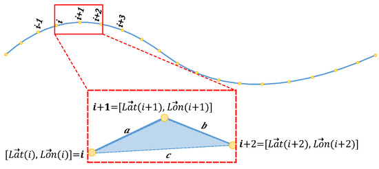
Figure 3.
Concept illustration of the triangle formed by three consecutive points of the railway track used to find the curvature radius.
The curvature radius of the point (i.e., ) is calculated by using (12), where is the triangle area, while a, b, and c are the triangle sides between the points i and , and , and and i, respectively, (see Figure 3). In turn, a, b, and c can be calculated from the latitude and longitude of each point as shown in (13), where D is the distance between two coordinate points defined by their longitude and latitude, and are the coordinates of the first point, and are the coordinates of the second point, R is the earth radius, and x is defined in (14).
This procedure is repeated from to to estimate the curvature radius from point 2 to point of the railway track, which are stored in a vector , where the first and last elements are defined as 0 m (i.e., m). Then, the points with a curvature radius greater than are neglected (i.e., assumed 0 m) as shown in Figure 4, since is a threshold used to determine if a section of the track is considered as a curve or not. The next step is to analyze the resulting vector to find the groups of consecutive points in with a radius less than and calculate the average of those radii (). Finally, is assigned to the point of the group with the least curvature radius.
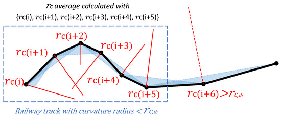
Figure 4.
Concept illustration of the calculation of and its assignment to a point of a group of consecutive points with .
Algorithm 1 summarizes the procedure to obtain with . The first loop calculates the curvature radius for each point of the curve by using the procedure described before, while the second loop identifies the groups of consecutive curvature radii greater than 0 m and less than along with their average values and assigns this value to the element of the group with the minimum curvature radius.
| Algorithm 1 Curvature radius () calculation |
|
3.4. Calculation of Speed, Elevation, Curvature, and Distance vs. Time Profiles
As mentioned in Section 2, it is necessary to know the speed, slope, and curvature radii vs. time profiles to calculate the forces acting on the train and the locomotive’s power. In some cases, these profiles can be obtained from railway operators, who have experimental data from the daily movements of the trains as well as the track data. Nevertheless, in zones where speed data or itineraries do not exist or are not open to the public, it could be generated from existing international or national regulations.
The first step to define a speed profile is to calculate the maximum theoretical speed that can be achieved by the train at each point of the track to generate a maximum speed profile (i.e., vs. ). Such a profile shows the restrictions for the speed profile generated from international and national regulations.
Each point of can be calculated from (1) assuming that the acceleration is 0 m/s, since the train moves at its maximum speed , which results in (15). Additionally, in (15) the locomotive force is calculated from the tractive and braking efforts profiles provided by the manufacturer, which show the maximum force (tractive or braking) produced by a locomotive for a particular speed. Equation (15) corresponds to the time instant where the train is at a particular point of the track, which means that and can be assumed constants while and are functions of . Therefore, for a point of the track is obtained by solving (15); then, the vs. profile is calculated by repeating this process for the points traced along the track.
The second step to determine a speed vs. time profile ( vs. ) is to define a speed vs. distance profile ( vs. ) considering the national and international regulations and limited by the vs. profile, where is a value less than 1 to avoid defining an element of at its maximum theoretical value. Such a profile has points and it is used along with to determine and, at the same time, the time profiles of the main variables: vs. , vs. , and vs. . It is important to mention that the subscript g in , , and represents the variable for each geographical point of the track given by , while the variables without the subscript (i.e., , , , and ) contain the information for each time of the journey given by .
The calculation of the time profiles is described in Algorithm 2, where the inputs and outputs are defined and , , , , and are auxiliary variables. The first If is used to calculate , which is the time required to move between two consecutive points of the track (i.e., and ) with the speed defined in the speed vs. distance profile () when such a speed is greater than 0 m/s.
| Algorithm 2 Calculation of , , , and |
|
The second If has two objectives: the first one is to calculate when m/s. The second objective is to determine to guarantee that the train stops at each station of the route, which is defined as 0 m/s in . This condition can be met if the numerical integration of the acceleration between two stops is 0 m/s. To achieve these two objectives the first step is to define and , which contain the elements of and between the last stop and the point before the actual stop, where the actual stop is identified if the condition m/s is true. Then, it is necessary to calculate the acceleration from and (i.e., ) and numerically integrate to obtain . The variables described before are illustrated in Figure 5, which shows an example of normalized speed and acceleration profiles.
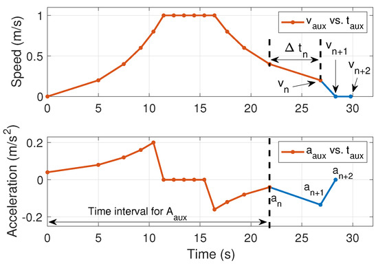
Figure 5.
Concept illustration of the calculation of when m/s to guarantee that the train stops.
The area under () is positive; therefore, the area under the last three points of the acceleration profile (see Figure 5) must be to obtain a null integration of the acceleration profile. To simplify this analysis, it is possible to add a point of 0 m/s to ( in Figure 5) to obtain a point of 0 m/s ( in Figure 5) in the acceleration profile. Then, equating the area under the points , , and to , it is possible to determine as shown in (16).
Considering that the procedure described above added an element to ( in Figure 5), it is also necessary to add an element to the other vectors (, , and ). The element is defined by adding to the previous time element of ( in Figure 5), where is a user-defined parameter. Moreover, the values of and for the time are defined as 0 rad and 0 m, respectively, since the train is not moving (see the end of Algorithm 2).
At this point, all the vectors required to calculate the train’s forces, power, and energy are available (, , , and ) to perform the steps defined in the flowchart in Figure 2
4. Results and Discussion
The proposed methodology was applied to two case studies to validate the calculations of the forces, power, and energy, defined in Section 2, as well as the estimation of the track information from satellite imagery, as described in Section 3.
The first case corresponds to the route from Alcazar de San Juan to Cartagena in Spain, which is used in [21] to calculate the energy consumption of different locomotives. This case study is aimed at validating the calculations introduced in Section 2 by comparing the total energy consumption reported in [21] with the one obtained with the proposed methodology for a Vossloh diesel-electric locomotive reference S-334.
The second case corresponded to the route from Chiriguaná to Santa Marta in Colombia, which is one of the few railways routes used in this country. In this case study, there was no available information on the route from the operators; hence, the proposed methodology was used to extract the route information from satellite imagery as described in Section 3. In this case, there was also no information about the locomotives and their loads; therefore, it was assumed that the same locomotive used in the first case study was moving on this route.
4.1. Case Study 1: Alcazar de San Juan to Cartagena–Spain
The first step in the methodology introduced in Figure 2 is to determine the main locomotive parameters. Some relevant parameters (such as nominal power, maximum speed, rail gauge, and weight) of the S-334 locomotive are introduced in Table 2, which are available in [34]. The methodology also requires the locomotive’s tractive effort and braking effort vs. speed profiles, which are presented in [34] and are introduced in Figure 6. Those figures were digitized and interpolated, as explained in Section 3, to estimate the tractive or braking force for the estimation of the maximum theoretical speed.
Table 2.
Vossloh S-334 diesel–electric locomotive characteristics.
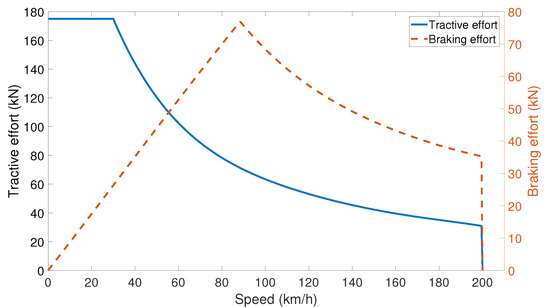
Figure 6.
Tractive effort vs. speed profile.
The parameters used for the calculations were the following: , , , and (Davis constants for all the coaches), , and (Davis constants for the locomotive) [21], , , , and a hotel load of .
In this case study, the railway track data were available in the plots reported in [21]; therefore, the elevation and speed profiles were obtained by digitizing the corresponding plots in [21]. Nevertheless, the detailed information on the curvature radii profile was difficult to obtain by digitizing the plot introduced in [21]; hence, the route from Alcazar de San Juan to Cartagena was traced in Google Earth with steps of 100 m, approximately, as shown in Figure 7. Applying the process introduced in Section 3.1, it was possible to obtain a plain-text file with 2216 points. Then, processing such file resulted in three vectors: , , and . Finally, the curvature radii profile could be calculated as explained in Section 3.3, with m [21], to obtain the vector and the profile shown in Figure 8.
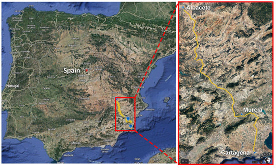
Figure 7.
Albacete–Cartagena route traced in Google Earth.
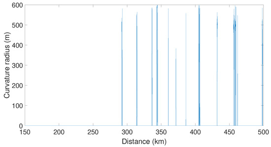
Figure 8.
Curvature radius profile calculated with the proposed methodology with m.
Afterward, the elevation vs. distance and speed vs. time profiles reported in [21] were digitized to obtain , , , and . This process resulted in the elevation and speed profiles reported in Figure 9 and Figure 10, respectively. The railway track information was completed by generating the other vectors (, , and ) by using the procedure described in Section 3; however, the slope profile was not plotted because this information was contained in the elevation profile.
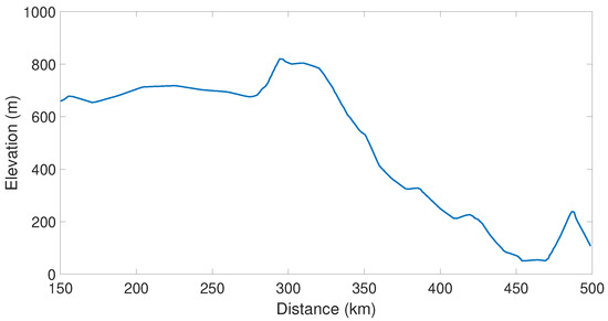
Figure 9.
Elevation profile digitized from [21] under CC BY 4.0 license.
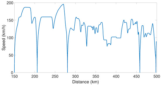
Figure 10.
Speed profile digitized from [21] under CC BY 4.0 license.
At this point, the locomotive and railway track information were available; hence, it was possible to calculate the forces at each point of the track as well as the power required by the locomotive to accelerate or decelerate the train. The plots shown in Figure 11a,b correspond to the powers provided in [21] and were estimated with the proposed methodology, respectively.
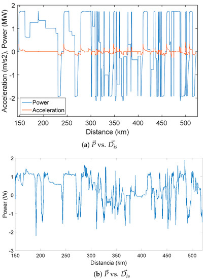
Figure 11.
(a) Power vs. distance profile reprinted from [21] under CC BY 4.0 license and (b) Power vs. distance profile obtained with the proposed methodology.
In those figures, it can be observed that the maximum values are similar (around MW), but the minimum values differ (MW for [21] and MW for the proposed methodology). Moreover, in both cases, the power takes positive and negative values according to the positive and negative slopes in the tracks, where positive slopes require positive power and energy consumption, while negative slopes result in negative power and energy generation due to the regenerative braking systems. Comparing Figure 11a,b, there are also differences in the points where the power is positive and negative. The differences described before are produced by unavoidable errors in the vectors , , and induced by the digitization process. Those errors in cause to be positive in [21] but negative in the digitized data in some points of the track, which produces a positive power in [21] but a negative power with the proposed procedure. Additionally, the digitization errors in the magnitudes of also produce differences in the magnitudes of , which affect the power profile and the energy estimation.
However, calculating the locomotive mechanical power and the total energy consumption by using the proposed methodology, the estimated total electrical energy was kWh, which was close to the total electrical energy provided in [21] ( kWh); therefore, the error in the energy consumption estimation was . These values show that the calculations introduced in Section 2 and the methodology described in Section 3 agree with the results reported in [21]; hence, the proposed methodology can be used to estimate the power and energy consumption of a particular locomotive in a given route.
4.2. Case Study 2: Chiriguaná–Santa Marta—Colombia
For this case study, it is important to mention that the route is not electrified; therefore, only diesel–electric locomotives must be considered. Following the methodology proposed in Section 3, the first step was to determine the main locomotive information. However, for this case study, it was assumed that the same model as in case study one (i.e., Vossloh S-334) was used; hence, the same parameters introduced in Section 4.1 were adopted including and s for the generation of the speed vs. time profile. In addition, the use of a diesel–electric locomotive S-594-2 was included in order to compare the energy performance of two locomotives on the same track. The main characteristics of the S-594-2 locomotive are related in Table 3 and its tractive and braking effort curves are illustrated in Figure 12.
Table 3.
CAF S-594-2 diesel–electric locomotive characteristics.
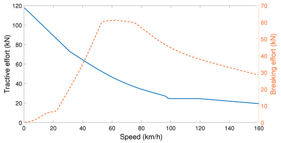
Figure 12.
Tractive vs. speed profiles.
The parameters used for the calculations of the S-594-2 locomotive were the following: T, , , and (Davis constants for all the coaches), , and (Davis constants for the locomotive) [21], , , , , s, and a hotel load of .
As mentioned before, the railway track information for the route Chiriguaná–Santa Marta from Figure 13 was not available; as consequence, the first step was to trace the route with lines of m approximately, using Google Earth, to obtain a KML file with the information of 2461 points. Then, the data were processed using GPS Visualizer to obtain a plain-text file with the information of elevation (from DEM using SRTM3 database NASA [35]), latitude, longitude, and distance between the consecutive points. From such a file, it was possible to generate the vectors , , , and .
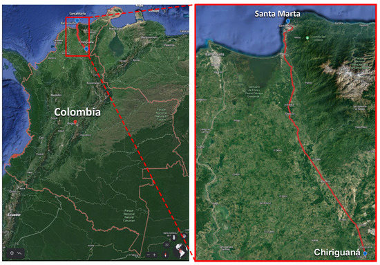
Figure 13.
Map of the railway track Chiriguaná–Santa Marta.
The vectors with the distances from the origin () and curvatures () were calculated as explained in Section 3.2 and Section 3.3 (with m), respectively. Nonetheless, the elevation had many changes in its values due to the estimation process performed from the DEM database. Those changes may suggest that the locomotive experiences changes in the slope sign every m, which is not realistic and introduces errors in the estimation of the locomotive power. Therefore, the elevation profile (i.e., vs. ) was smoothed by using a moving average filter with five samples. The original and filtered elevation profiles are introduced in Figure 14, where it can be observed that the filtered profile shows a significant reduction in the number of changes in the elevation regarding the distance.
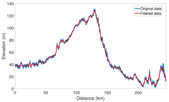
Figure 14.
Original and filtered elevation profiles of the route Chiriguaná–Santa Marta.
Now, the curvature radii vs. distance profile was calculated by using Algorithm 1, which produced the vector . The location and radii of the curves along the route are presented in Figure 15. This figure was obtained by plotting against . In this case, 32 curves were identified with m, where the minimum curvature radius was 255 m.
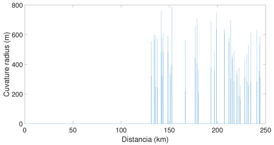
Figure 15.
Location of curves and their radii of the route Chiriguaná–Santa Marta.
Given the lack of information on speed profiles in the analyzed route, the proposed speed vs. distance profile ( vs. ) assumed that the locomotive moved at the maximum speed allowed by the Colombian rail traffic regulation [36]. This regulation defines a maximum speed of km/h in residential zones and km/h in open zones. Additionally, the speed profile also considered two theoretical stations in two towns (Bosconia and Fundación), where the speed goes down to km/h. Those stations are located at km (Bosconia) and km (Fundación) from the Chiriguaná station. The maximum speed profile ( vs. ) was also calculated as described in Section 3.4 to determine the speed restrictions. For the train with the S-334 locomotive, was greater than the maximum speeds defined by the Colombian regulation at all the points of the track; however, this was not the case for the same train with the S-594-2 locomotive. The vs. and vs. profiles used for this case study are reported in Figure 16 and Figure 17 for the S-334 and S-594-2 locomotives, respectively. It is worth noting that is considered to limit the vs. for S-334 and S-594-2 locomotives; hence, the speed profile presented in Figure 16 is not affected by , while the one presented in Figure 17 is defined by for most of the route.
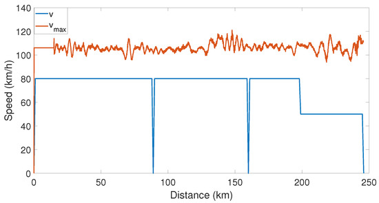
Figure 16.
Speed profile of the route Chiriguaná–Santa Marta with S-334 locomotive.
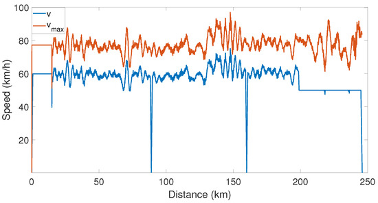
Figure 17.
Speed profile of the route Chiriguaná–Santa Marta with S-594-2 locomotive.
Using Algorithm 2 resulted in , , , , and ; hence, at this point, it was possible to calculate the mechanical power of the train at each point of the route () by using (6). The estimated power profile was obtained by combining and , as shown in Figure 18, which was used to calculate the total energy consumed by the locomotive according to (7). Moreover, during the deceleration and in negative slopes, the mechanical power is negative, and such power represents the theoretical energy that could be generated, which was computed using (9). Finally, the electrical energy demand was computed from (8), which represents the energy needed by traction motors to move along the studied path. Those values are compiled in Table 4 for the two studied locomotives, as well as the time required to complete the route.
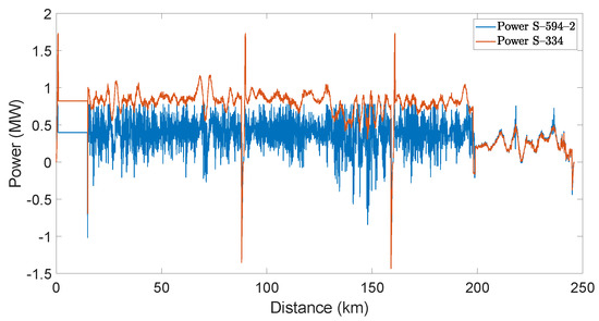
Figure 18.
Power vs. distance profile, Chiriguaná–Santa Marta route.
Table 4.
Simulation results for the studied locomotives.
Figure 18 also shows that the maximum and minimum values of the mechanical power for the S-334 locomotive are MW and MW, respectively; and for the S-594-2 locomotive the maximum and minimum values are MW and MW, respectively, which is in agreement with the mechanical power that diesel motors can deliver to each locomotive. Moreover, for the S-334 locomotive, it can be observed that the required power peaks are experienced at the moments of braking and starting. On the other hand, it is possible to observe that in most parts of the route there is a positive consumption for the S-334 locomotive, so the potential generated energy is less than that of the S-594-2 locomotive. In the case of the S-594-2 locomotive, it can be observed that the power changes between negative and positive values due to the variations of the speed profile (see Figure 17).
These results show that both locomotives can move the train along the route with some differences. On the one hand, the S-334 locomotive can reach the maximum speed defined by the Colombian regulations and complete the route in h, which requires an electrical energy consumption of kWh and has a potential to generate kWh. On the other hand, the maximum power of the S-594-2 locomotive does not allow reaching the maximum speed defined by the Colombian regulations; as consequence, regarding the S-334 locomotive, the time to complete the route is longer ( h), but the electrical energy required is smaller ( kWh) and the potential energy generation bigger ( kWh).
The results of the case studies presented in this section show the applicability of the proposed methodology to estimate the power and energy consumed by a locomotive when the track information is not complete or not available. Therefore, the proposed methodology can be used for different applications, such as assessing the energy consumption (E) of different locomotives for a given route to select the best option; or estimating the power consumed by the locomotive at each point of the route as well as the potential energy that can be generated (), to inject into the grid or to be used in energy storage systems.
5. Conclusions
A methodology for estimating the energy consumption and the potential energy generation of a locomotive, when the railway track information is not available or incomplete, was presented in this paper. The methodology started by extracting the main technical information of the locomotive to be analyzed. Then, the railroad track was traced in Google Earth with 100 m steps, from which longitude, latitude, and elevation data were extracted to estimate the track’s slope and curvature profiles. Moreover, the methodology proposed to create a speed profile based on the data provided by the track operator or the regulations of the country where the analysis is to be implemented, but considering the maximum theoretical speed at each point of the track. The estimation of the locomotive power at each point of the route was generated with the collected information to finally calculate the energy consumed. Hence, the proposed methodology can help railway companies determine the best locomotive for a given route during the period of planning, construction, and operation, which may positively affect the economic, environmental, and other indicators of a railway project.
This methodology was initially tested on a Spanish railway route, for which the data published by other authors were available. Likewise, the results were compared between a model with sufficient information and the proposed methodology to estimate the energy consumption of a train, presenting an error of between both data. This error was attributed to the digitization of the information taken from the case in Spain. Finally, the methodology was applied to one of the Colombian railroads, the results providing sufficient information to determine the energy to be provided in the proposed trajectory for a possible upgrade of the locomotive technology and planning of the railway infrastructure and energy generation systems. Two different diesel–electric locomotives were compared for the case study in Colombia. Such a comparison showed that the locomotive power limited the maximum speed that could be reached by a train on the studied route, which translated into longer traveling times for the same load. Moreover, the energy consumed and generated by the two locomotives was significantly different, which showed that the proposed methodology could be used to evaluate different technologies for a particular application.
In future work, we propose to extend the data collection to other rail trajectories without public information and to identify tracks in a country where such information is not available. In this way, it will be possible to estimate the energy consumption and propose technological upgrades to improve freight and passenger transportation in a region. Moreover, it would also be interesting to use the proposed procedure for optimization problems such as the reduction of emissions, the reduction of fuel consumption, or the reduction of the charging/discharging cycles of energy storage systems.
Author Contributions
M.A.R.-C., D.A.H.-J., J.D.B.-R., J.P.V.-C. and K.S.M.-V. contributed equally in the processes associated to the paper: conceptualization, methodology, software, validation, writing—original draft preparation, writing—review and editing. All authors have read and agreed to the published version of the manuscript.
Funding
This research was funded by UPME and Ministerio de Ciencia, Tecnología e Innovación (project code 2243-879-79863), Instituto Tecnológico Metropolitano (project code RC 80740-034-2021), and Universidad Nacional de Colombia (project code HERMES 50648) under the project “FERROFLUVIAL 4.0—Plan de Investigación para la Evaluación y Priorización de Tecnologías Orientadas a la Electromovilidad y su Penetración e Impactos en el Fortalecimiento de Encadenamientos Productivos de Colombia en sus Modos Férreo y Fluvial”.
Institutional Review Board Statement
Not applicable.
Informed Consent Statement
Not applicable.
Data Availability Statement
The data used in this study are reported in the paper’s figures and tables.
Acknowledgments
Ministerio de Ciencia, Tecnología e Innovación (Minciencias), Instituto Tecnológico Metropolitano, and Universidad Nacional de Colombia.
Conflicts of Interest
The authors declare no conflict of interest.
References
- Bailey, J. The steam age—Evolution of steam engines and the 1st steam locomotive. In Inventive Geniuses Who Changed the World: Fifty-Three Great British Scientists and Engineers and Five Centuries of Innovation; Springer International Publishing: Cham, Switzerland, 2022; pp. 23–36. [Google Scholar] [CrossRef]
- Mayet, C.; Pouget, J.; Bouscayrol, A.; Lhomme, W. Influence of an energy storage system on the energy consumption of a diesel-electric locomotive. IEEE Trans. Veh. Technol. 2013, 63, 1032–1040. [Google Scholar] [CrossRef]
- Mandić, M.; Uglešić, I.; Milardić, V. Method for optimization of energy consumption of electrical trains. Int. Rev. Electr. Eng. 2011, 6, 292–299. [Google Scholar]
- Morais, V.A.; Afonso, J.L.; Martins, A.P. Modeling and validation of the dynamics and energy consumption for train simulation. In Proceedings of the International Conference on Intelligent Systems (IS), Wrocław, Poland, 17–18 September 2018; pp. 288–295. [Google Scholar]
- Pappaterra, M.J.; Flammini, F.; Vittorini, V.; Bešinović, N. A Systematic Review of Artificial Intelligence Public Datasets for Railway Applications. Infrastructures 2021, 6, 136. [Google Scholar] [CrossRef]
- Komyakov, A.; Nikiforov, M.; Erbes, V.; Cheremisin, V.; Ivanchenko, V. Construction of electricity consumption mathematical models on railway transport used artificial neural network and fuzzy neural network. In Proceedings of the 16th International Conference on Environment and Electrical Engineering (EEEIC), Florence, Italy, 6–10 June 2016; pp. 1–4. [Google Scholar]
- Liu, J. Calculation and analysis of energy consumption of Chinese national rail transport. Int. J. Energy Sect. Manag. 2018, 12, 189–200. [Google Scholar] [CrossRef]
- Biliaiev, M.M.; Rusakova, T.I.; Kozachyna, V.A.; Berlov, O.V.; Poltoratska, V.M.; Yakubovska, Z.M. Simulation of environmental pollution from diesel locomotive. IOP Conf. Ser. Mater. Sci. Eng. 2020, 985, 012019. [Google Scholar] [CrossRef]
- Carvalhaes, B.B.; de Alvarenga Rosa, R.; Márcio de Almeida, D.; Ribeiro, G.M. A method to measure the eco-efficiency of diesel locomotive. Transp. Res. Part D Transp. Environ. 2017, 51, 29–42. [Google Scholar] [CrossRef]
- Cipek, M.; Pavković, D.; Kljaić, Z.; Mlinarić, T.J. Assessment of battery-hybrid diesel-electric locomotive fuel savings and emission reduction potentials based on a realistic mountainous rail route. Energy 2019, 173, 1154–1171. [Google Scholar] [CrossRef]
- Cipek, M.; Pavković, D.; Krznar, M.; Kljaić, Z.; Mlinarić, T.J. Comparative analysis of conventional diesel-electric and hypothetical battery-electric heavy haul locomotive operation in terms of fuel savings and emissions reduction potentials. Energy 2021, 232, 121097. [Google Scholar] [CrossRef]
- Rodriguez, R.; Trovão, J.P.F.; Solano, J. Fuzzy logic-model predictive control energy management strategy for a dual-mode locomotive. Energy Convers. Manag. 2022, 253, 115111. [Google Scholar] [CrossRef]
- Jia, C.; Qiao, W.; Qu, L. A cost-oriented control strategy for energy management of a dual-mode locomotive. In Proceedings of the IEEE Vehicle Power and Propulsion Conference (VPPC), Hanoi, Vietnam, 14–17 October 2019; pp. 1–6. [Google Scholar]
- Mendoza, D.S.; Acevedo, P.; Jaimes, J.S.; Solano, J. Energy management of a dual-mode locomotive based on the energy sources characteristics. In Proceedings of the IEEE Vehicle Power and Propulsion Conference (VPPC), Hanoi, Vietnam, 14–17 October 2019; pp. 1–4. [Google Scholar]
- Macian, V.; Guardiola, C.; Pla, B.; Reig, A. Application and benchmarking of a direct method to optimize the fuel consumption of a diesel electric locomotive. Proc. Inst. Mech. Eng. Part F J. Rail Rapid Transit 2018, 232, 2272–2289. [Google Scholar] [CrossRef]
- Alzhanov, B.; Nataliya, S. The Methodology for Energy Efficiency on Electric Locomotive Traction for the Heaviest and Longest Trains in the Operation of the Kazakh Railway. Int. J. Railw. 2017, 10, 30–33. [Google Scholar] [CrossRef]
- Wu, Q.; Spiryagin, M.; Cole, C. Train energy simulation with locomotive adhesion model. Railw. Eng. Sci. 2020, 28, 75–84. [Google Scholar] [CrossRef] [Green Version]
- Lindgreen, E.; Sorenson, S. Simulation of Energy Consumption and Emissions from Rail Traffic; MEK-ET-2005-04; Technical University of Denmark—Department of Mechanical Engineering: Copenhagen, Denmark, 2005. [Google Scholar]
- Zarifian, A.A.; Kolpahchyan, P.G. Computer modeling of electric locomotive as controlled electromechanical system. Multibody Syst. Dyn. 2009, 22, 425–436. [Google Scholar] [CrossRef]
- Liu, J.; Guo, H.; Yu, Y. Research on the Cooperative Train Control Strategy to Reduce Energy Consumption. IEEE Trans. Intell. Transp. Syst. 2017, 18, 1134–1142. [Google Scholar] [CrossRef]
- García-Garre, A.; Gabaldón, A. Analysis, evaluation and simulation of railway diesel-electric and hybrid units as distributed energy resources. Appl. Sci. 2019, 9, 3605. [Google Scholar] [CrossRef] [Green Version]
- Bakhtiyorovich, K.N.; Shomansurovich, T.S. Application of Modern Information Technologies and Software Tools in the Design of Railways. Int. J. Discov. Innov. Appl. Sci. 2021, 1, 1–3. [Google Scholar]
- Arruda, H.; Ohashi, O.; Ferreira, J.; De Souza, C.; Pessin, G. Exploiting machine learning for the identification of locomotives’ position in large freight trains. Appl. Artif. Intell. 2019, 33, 902–912. [Google Scholar] [CrossRef]
- Prapulla, S.; Rao, S.N.; Herur, V.A. Road quality analysis and mapping for faster and safer travel. In Proceedings of the International Conference on Energy, Communication, Data Analytics and Soft Computing (ICECDS), Chennai, India, 1–2 August 2017; pp. 2487–2490. [Google Scholar]
- Franco, A. Road Curvature Calculation. 2022. Available online: https://www.adamfranco.com/2012/12/05/curvature-py/ (accessed on 5 June 2022).
- Resende, L.P.; Silva, L.T.; Tomim, M.A. Railway trajectory modeling for simulation of locomotives drive systems. In Proceedings of the Brazilian Power Electronics Conference (COBEP), Juiz de Fora, Brazil, 19–22 November 2017; pp. 1–8. [Google Scholar]
- Lu, Q.; He, B.; Wu, M.; Zhang, Z.; Luo, J.; Zhang, Y.; He, R.; Wang, K. Establishment and analysis of energy consumption model of heavy-haul train on large long slope. Energies 2018, 11, 965. [Google Scholar] [CrossRef] [Green Version]
- SUSTRAIL Consortium. Hybrid Locomotive Deliverable D3.2.1; Technical Report; 2014. Available online: https://www.sustrail.eu/IMG/pdf/d3.2-v1-hybrid_locomotive-final_version.pdf (accessed on 5 June 2022).
- Andryushchenko, A.; Kolpahchyan, P.; Zarifyan, A. Reduction of electric locomotive’s energy consumption by scalable tractive power control. Transp. Probl. 2018, 13, 103–110. [Google Scholar] [CrossRef] [Green Version]
- Fayad, A.; Ibrahim, H.; Ilinca, A.; Sattarpanah Karganroudi, S.; Issa, M. Energy Recovering Using Regenerative Braking in Diesel-Electric Passenger Trains: Economical and Technical Analysis of Fuel Savings and GHG Emission Reductions. Energies 2022, 15, 37. [Google Scholar] [CrossRef]
- Agenjos, E.; Gabaldon, A.; Franco, F.; Molina, R.; Valero, S.; Ortiz, M.; Gabaldon, R. Energy efficiency in railways: Energy storage and electric generation in diesel electric locomotives. In Proceedings of the IET Conference, Prague, Czech Republic, 8–11 June 2009; p. 402. [Google Scholar] [CrossRef] [Green Version]
- Quintana, J.J.; Ramos, A.; Diaz, M.; Nuez, I. Energy efficiency analysis as a function of the working voltages in supercapacitors. Energy 2021, 230, 120689. [Google Scholar] [CrossRef]
- Leydesdorff, L.; Persson, O. Mapping the geography of science: Distribution patterns and networks of relations among cities and institutes. J. Am. Soc. Inf. Sci. Technol. 2010, 61, 1622–1634. [Google Scholar] [CrossRef] [Green Version]
- Renfe. Manual de Conducción Locomotora Diesel ElÉctrica S334. 2006. Available online: https://docplayer.es/93934747-Manual-de-conduccion-s-334.html (accessed on 5 June 2022).
- NASA. NASA Shuttle Radar Topography Mission, Version 3, 3 arc Second. NASA EOSDIS Land Processes DAAC, USGS Earth Resources Observation and Science (EROS) Center, Sioux Falls, South Dakota. 2013. Available online: https://lpdaac.usgs.gov (accessed on 28 October 2021).
- Ministerio de Transporte de Colombia. Manual de Normatividad férrea Parte I; Ministerio de Transporte de Colombia: Bogotá, Colombia, 2013.
Publisher’s Note: MDPI stays neutral with regard to jurisdictional claims in published maps and institutional affiliations. |
© 2022 by the authors. Licensee MDPI, Basel, Switzerland. This article is an open access article distributed under the terms and conditions of the Creative Commons Attribution (CC BY) license (https://creativecommons.org/licenses/by/4.0/).