Research on Calculation Method for Discharge Capacity of Draining Well in Tailing Ponds Based on “Simplification-Fitting” Method

Abstract

The existing empirical formulas concerning draining systems are complex in their expression: there are difficulties in locating the intersection point among different flow patterns and parameters vary depending on the water level, resulting in a large amount of data to be processed and low calculation efficiency. To solve these problems, a “simplification-fitting” method was proposed herein to calculate the discharge capacity of a window-type draining well, and optimal and reasonable locations were selected as discrete points of water level to deduce the increasing progressive relationship of free flow discharge capacity among discrete points according to the window size and longitudinal layout of window-type draining wells. Additionally, the algorithm simplified the discharge formulas of half-pressure flow and pressure flow and defined the convergence criteria for water level-discharge capacity to further simplify the expression of pressure flow. The comparison and contrast between the simplified calculation method and empirical formula method show that the method herein is of high precision. It is able to resolve the shortcomings of the traditional theoretical formula method in solving the discharge capacity curve of a window-type draining well and simplify the algorithm integration.

1. Introduction

A tailing pond stands as a critical facility affiliated with mines. Its safe operation is vital to the daily production of mining companies and the safety of the downstream area. The flood-discharging system of the tailing pond serves as an essential approach to discharge catchment water on the slope surface and to supply mining company with production water [1,2].

An insufficient discharge capacity in this system will increase the risk of flood overflow atop the tailing pond and simultaneously cause the water level in the tailing pond to be higher than its safety control value, thus driving the saturation line to exceed the safety threshold, increasing the seepage, deformation and damage risks and even directly inducing the dam break [3,4].

It is a critical measure to guarantee the safe operation of tailing ponds by specifying the permissible water level in tailing pond reservoir through flood routing calculation before the flood season [5]. Li [6] highlighted that the drainage system has the characteristics of multiple inlets and complex flow patterns, and that the calculation of the discharge capacity of a flood-discharging system is a crucial step in flood routing [6]. Its calculation accuracy directly influences the precision of the calculation results of the flood routing program. Therefore, scholars conducted many analyses and discussions to research the variation pattern and the specific quantity of discharge capacity of the flood-discharging system in a tailing pond. Li [7] and Tan [8] summarized the problems existing in the hydraulic calculation of discharge system in a tailing pond, and suggested that free flow is recommended to estimate the discharge system, especially the combined patterns discharge system. As the primary method of studying the hydraulic characteristics of the flood-discharging system, the hydraulic model test was taken as the basic method for researching the changing process of discharge capacity in complex flood-discharging systems. Liu [9] carried out a hydraulic experimental model to research the flow characteristics of the curved section of the spillway tunnel, and found that the flow pattern and its change tendency was the basic influence factor for the designing of the tunnel. Wang [10] studied the influence of shaft depth on the discharge capacity through a typical tailing dam heightening project, and established the fitting function relation between discharge and shaft depth. Han [11] and Du [12] carried out an experimental model based on the principle of similarity to simulate the process of the water level rising in a tailing pond and to obtain the complex ternary water flow movement laws, they found that the angle of the turning can be adjusted to reduce the backwater height. Djillali [13] proposed a new design for the shaft spillway, replacing the circular section with a polygonal configuration of 12 sections, thus making the hydraulic structure more reliable. Fraga [14] proposed a model under unsteady part-full and pressure flow conditions. Zakwan [15] established the relationship between the coefficient and flow of side weir. Ebtehaj [16] recommended a multi-objective method for the prediction of the side weir discharge coefficients. Sen [17] used a stabilized finite-element method to discrete the conservation equations of incompressible fluid flow in two dimensions. Dennis [18] suggested the small to moderate values of the Reynolds number for higher accuracy. These research results were subject to theoretical generalization and analysis, and applied to practical projects.

In complicated and unconventional flood-discharging systems, numerical simulation methods can be adopted as a simple, cheap, and reliable means of analyzing the hydraulic variation characteristics. Mo [19], Zhao [20] and Bao [21] carried out the numerical simulation analysis of different discharge systems; in these simulations, the flow pattern, velocity distribution, water surface profile and other hydraulic characteristics were analyzed, and the simulation results showed that the use of numerical simulation is of high accuracy. The numerical simulation software adopted includes Flow-3D, 3D VOF model, Fluent, etc. Three-dimensional hydraulic simulation is usually adopted to modify the parameters of theoretical formulas, especially when the design of a discharge system is unconventional and thus theoretical formulas cannot accurately calculate the discharge capacity. For example, Wang [22] adopted Flow-3D to simulate the downstream of the sluices; Ling [23] built a 3D water quality model coupled VOF method and the k-ε turbulence model; Yi [24] chose Flow-3D to simulate the water characteristic of window type, frame type and chute type water-discharge system, respectively. Yu [25] simulated the flow in a siphon-shaped overflow tower under both steady and unsteady flow conditions using CFD. However, calculation results may deviate from actual projects because some basic assumptions were adopted in numerical simulation or the selected parameters are unreliable. In this situation, a method combining numerical simulation with the model test can be adopted [26] to invert calculating parameters for a numerical simulation with model test results. Then, simulation results more consistent with reality can be obtained. Meanwhile, repeated numerical simulations can be exploited to predict the discharge results under multiple operating conditions. The analysis combining the empirical calculation formula of discharge capacity with monitoring results also serves as a key research method. Based on the real-time monitoring results of water level and discharge capacity, the parameters of the empirical calculation formula can be modified, and a more accurate prediction formula can be obtained [27]. In addition to the aforementioned methods, the empirical formula and the numerical simulation results of computational fluid dynamics have been compared to achieve mutual verification and calibration. For example, Wu [28] compared the calculation results of the empirical formula and computational fluid dynamics flow simulation (CFD), and found that the discharge capacity of half-pressure flow calculated by CFD method is higher but more reasonable than that of the empirical formula method. Ning [29] found that LUSGS preconditioning is slightly better than the ILU preconditioning. Liu [30] and Dang [31] stated that chute plate type, chute slope, water head and flow patterns on flow capacity should be adequately considered in the design stage. These achievements lay a theoretical basis for the optimal design of the flood-discharging system of tailing ponds [32,33,34,35].

In recent years, as the information construction rapidly progresses and develops, it has become a development trend to establish the flood routing algorithm system for tailing ponds based on the dynamic monitoring data of rainfall and water level so as to realize a real-time analysis and calculation on flood routing for tailing ponds. This trend has put forward new requirements on the accuracy and efficiency of hydraulic calculation concerning flood-discharging systems [36,37,38]. On this basis, the “window-type draining well plus tunnel/draining pipe” draining system was chosen herein to research the algorithm for discharge capacity.

Theoretical Calculation Formulas

According to the References for Tailing Pond Design [39], the working conditions of a “window-type draining well plus tunnel/draining pipe” flood-discharging system vary in function of the size of the discharge water head, which can be divided into free flow, half-pressure flow and pressure flow. Their specific calculation methods are listed in

Table 1. Theoretical calculation formulas of “window-type draining well plus tunnel/draining pipe” flood-discharging system.

Working Conditions	Calculation Formulas
Free Flow (a) When the water level is between two layers of windows. (b) When the water level is in the window position.	$Q_a=Q_2=2.7n_c{\omega }_c\sum \sqrt{H_i}$ $Q_b=Q_1+Q_2$ $\mathrm{For} \mathrm{square} \mathrm{orifice}, Q_1=1.8n_c\epsilon b_c{H}_0{}^{1.5}$ $\mathrm{For} \mathrm{round} \mathrm{orifice}, Q_1\approx n_{c}A{D}_c^{2.5}$	(1)
Half-Pressure Flow	$Q=\phi F_s\sqrt{2gH}$ $\phi =\frac{1}{\sqrt{1+{\lambda }_j\frac{l}{d}{f}_1^2+{\zeta }_1{f}_2^2+{\zeta }_2+2{\zeta }_3{f}_1^2}}$	(2)
Pressure Flow	$Q=\mu F_s\sqrt{2g{H}_z}$ $\mu =\frac{1}{\sqrt{1+\sum {\lambda }_g\frac{L}{D}{f}_3^2+\sum \zeta f_3^2+{\zeta }_1{f}_4^2+{\zeta }_2{f}_9^2+2{\zeta }_3{f}_5^2}}$	(3)

Notes: Descriptions of symbols in the table.

:

• H_i—Discharging water head calculated at the working window fully submerged on the ith floor, m;
• H₀—Discharging water head at the working window not submerged on the ith floor, m;
• H—Water head calculated, the difference between the water level in the pond and the elevation of the inlet section center of the draining pipe, m;
• H_z—Water head calculated, the difference between the water level in the pond and the elevation of downstream outlet section center of the draining pipe, or the height difference between the water level in the pond and the level of tail water when there is water downstream, m:
• ${\omega }_c$—The area of one draining window, m²;
• ${\omega }_s$—Flow shrinkage area at the wellhead, m², ${\omega }_s={\epsilon }_b{\omega }_j$;
• $\omega$—The total window area within the water depth range, m²;
• ${\omega }_j$—Cross-section area of draining well shaft, m²;
• ${\omega }_1$—Total window area of draining well, m²;
• ${\omega }_2$—External surface area of draining well shaft, m²;
• $F_s$—Water flow shrinkage area at draining pipe inlet, m², F_s = ε_bF_e;
• $F_e$—Sectional area of draining pipe inlet, m²;
• $F_x$—Sectional area of downstream outlet of draining pipe, m²;
• $F_g$—Sectional area of calculating pipe segment of draining pipe, m²;
• $\zeta$—Local head loss coefficient of draining pipeline, including angle, bifurcation, section change, etc., which can be obtained by referring to relevant tables;
• ${\zeta }_0$—Coefficient, related to the shape of gate pier head;
• ${\zeta }_1$—Local head loss coefficient of draining window, ${\zeta }_1={\left(1.707\frac{{\omega }_1}{{\omega }_2}\right)}^2$;
• ${\zeta }_2$—Local head loss coefficient of draining pipe inlet, rectangular entrance ${\zeta }_2$ = 0.5, fillet angular or oblique angular entrance ${\zeta }_2$ = 0.2~0.25, flare opening entrance ${\zeta }_2$ = 0.1~0.2;
• ${\zeta }_3$—Local head loss coefficient of water diversion in a draining well;
• $\epsilon$—Lateral contraction coefficient, $\epsilon =1-\frac{0.25{\zeta }_0{H}_h}{b_c}$;
• ${\epsilon }_b$—Sectional sudden contraction coefficient;
• $d$—Inner diameter of draining well, m, but if the well shape is not circular, $d=4R_j$;
• $D$—Inner diameter of calculating pipe segment, m, but if the pipe is not circular, $D=4R_g$;
• $L$—The calculated length of the pipe segment of draining pipe (when there is no change in the cross section, the length is the full length of pipeline), m;
• $A$—Coefficient, obtained with reference to relevant tables and based on $\frac{H_0}{D_c}$;
• $R_g$—Hydraulic radius of calculating pipe segment of draining pipe, m;
• $R_j$—Hydraulic radius of shaft section of drainage well, m;
• $D_c$—Draining well diameter, m;
• $b_c$—Width of one draining window, m;
• $n_c$—Number of draining windows on the same cross-section;
• ${\lambda }_j$—Frictional head loss coefficient of draining well, $\lambda =\frac{8g}{C^2}$;
• ${\lambda }_g$—Frictional head loss coefficient of draining window, $\lambda =\frac{8g}{C^2}$;
• C—Chezy coefficient, with reference to relevant documents and according to $n$ and R; $n$—Pipe wall roughness coefficient;

$$f_1=\frac{F_s}{{\omega }_j}; f_2=\frac{F_s}{\omega }; f_3=\frac{F_x}{F_g}; f_4=\frac{F_x}{\omega }; f_5=\frac{F_x}{{\omega }_j}; f_9=\frac{F_x}{F_e}$$

There will be the following problems when these formulas are adopted to calculate the discharge capacity:

(1)

In the free discharge stage, as the water level increases, there will be three combined flow regimes—the weir flow, the orifice flow, and the weir flow + orifice flow. These correspond to the water levels within the elevation range of the first window, between two layers of windows, and within the elevation ranges of windows other than the first window. Therefore, the relationship between the water level and window position should be judged whenever necessary in the calculation. The discharge capacity under three flow regimes can be obtained by choosing and combining reasonable formulas, thus resulting in a complicated calculation process.

(2)

There are many parameters, iterations among parameters and applications in this method, and the water level is also closely involved. Furthermore, fluctuations in water level result in constant changes in calculation parameters.

(3)

The empirical formula method has to locate the intersection point among the free flow curve, the half-pressure flow curve, and the pressure flow curve, and choose the discharge capacity calculation formula according to the relative position relationship between the actual water level and the intersection point. This requirement will bring about logical difficulties in algorithm integration.

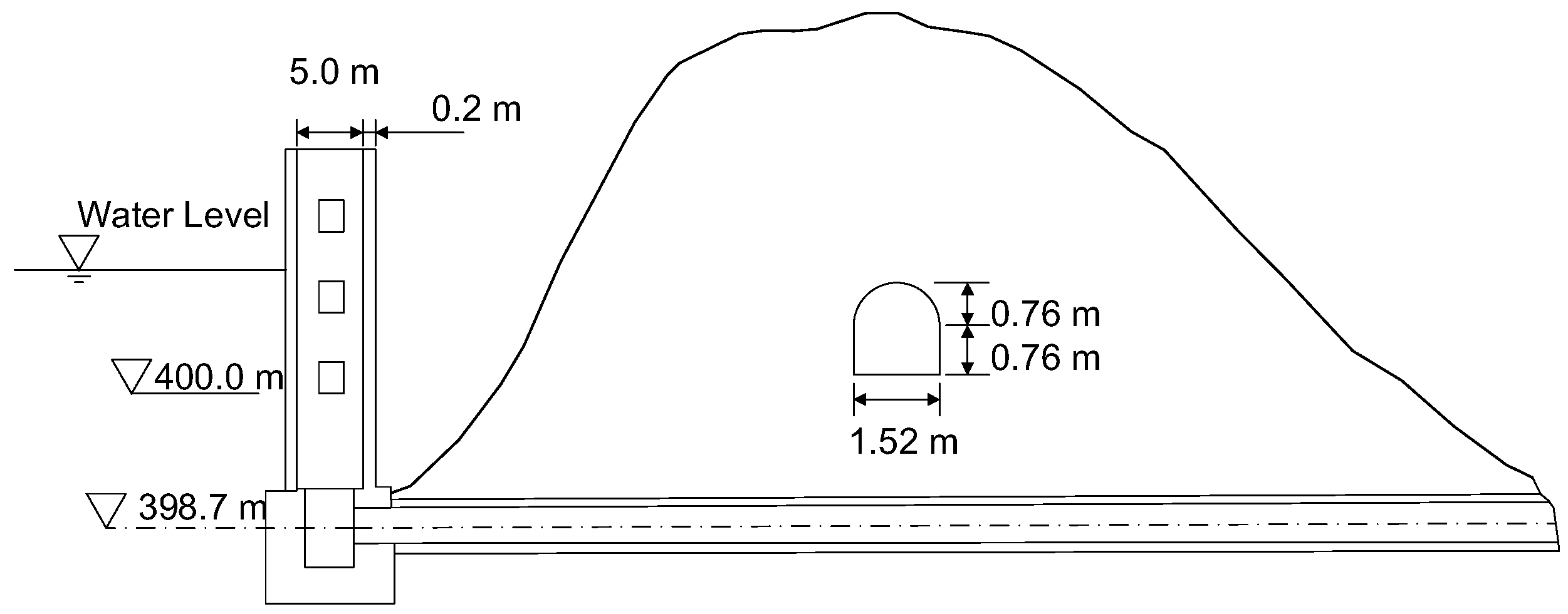
In order to overcome the shortcomings of the existing theoretical calculation method, a simplified calculation method needs to be proposed to enhance the significance of discharge capacity calculation efficiency of the “window-type draining well plus tunnel/draining pipe” flood-discharging system, thus realizing algorithm simplification and program-based treatment, and delivering a higher calculation accuracy.

The literature review showed a very small number of studies similar to the simplification-fitting method. Discharge capacity calculation is critical to flood routing calculation, which is an important measurement to guarantee the safety of the tailing pond. However, the theoretical formulas recommended in books are enormously complex in expression, and are thus those algorithm cannot be implemented to flood the routing calculation program. Therefore, this article presents for the first time research on a simplification method of calculation equations for a discharge system in tailing pond. The proposed method determines discrete water level points according to the shape, size, and spacing of windows. The simplified formulas for free flow, half-pressure flow, and pressure flow were obtained through a specific discrete method. The discrete values calculated by the simplified formula were adopted to fit those data, and to obtain the discharge capacity value on a random water level. A series of comparative analyses was carried out during the free flow stage, half-pressure flow stage, and pressure flow stage, respectively, the purpose of which was to verify the accuracy of the simplified algorithm proposed in this study. The obtained analysis results indicate that the proposed simplification method made it possible for discharge algorithm computer integration with the flood routing program in a low-cost, high-efficient and steady way.

2. Physical Model

In the window-type draining system in a tailing pond shown in Figure 1 [39], there are six draining windows on each floor of the well; the window size is 0.5 × 0.5 m; the clear vertical distance between windows is 0.2 m; the inner diameter of draining well is 5.0 m; the draining well wall is as thick as 0.2 m; the elevation of cover plate is 400.0 m; the pedestal elevation is 398.7 m; the draining tunnel has the shape of a horseshoe, whose bottom is as wide as 1.52 m; and the height of the straight wall is 0.76 m. The curve of the relationship between the discharge capacity of this draining system and the water level in the tailing reservoir was calculated.

3. Method

A unique discrete point selection method was proposed based on a systematical summary of the empirical calculation formula of a window-type draining well to simplify the formula in the free discharge stage. Simultaneously, calculation parameters in half-pressure flow and pressure flow stages were simplified according to the characteristics of draining wells in tailing ponds to simplify calculation expressions. The flow chart of the simplified algorithm for the discharge capacity of window-type draining wells is shown in Figure 2.

The specific “simplification-fitting” calculation processes are shown as follows:

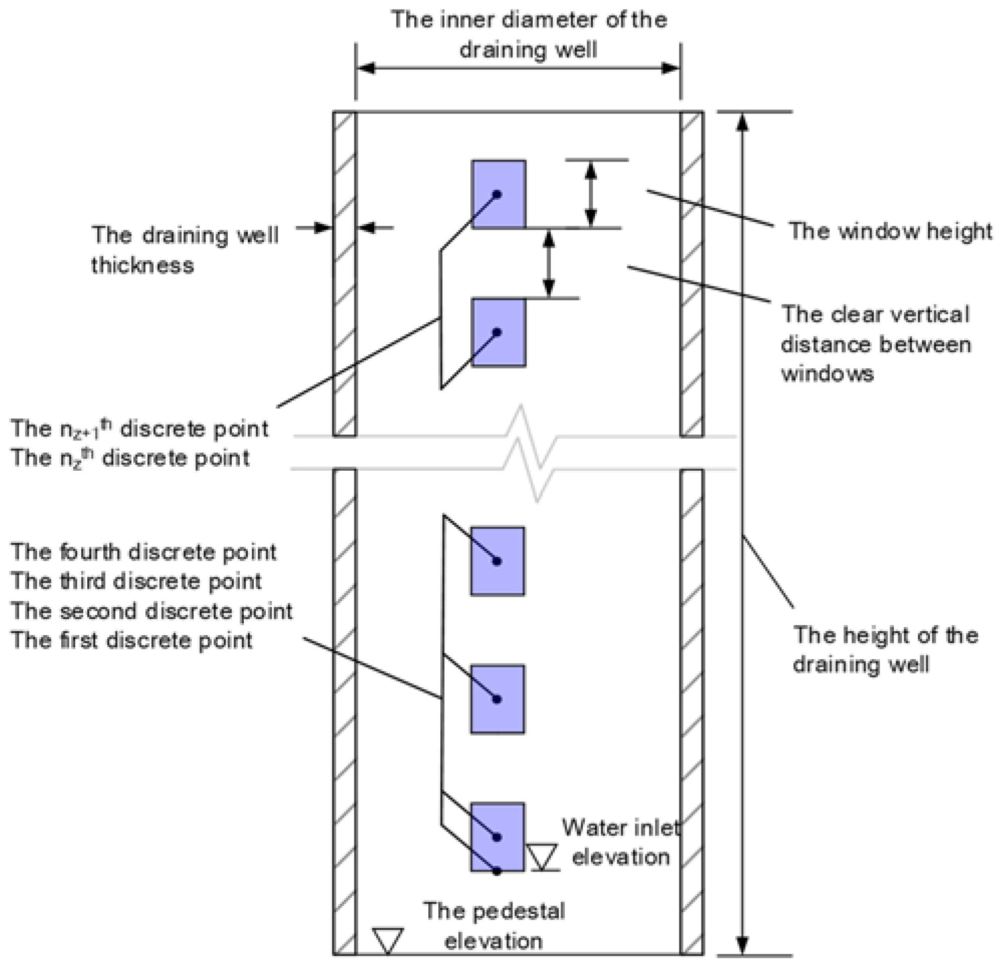
• Step 1. The coordinates of discrete points for the simplified algorithm were obtained according to the dimension parameters of the window-type draining well input, including the window number on the same longitudinal section n_z, the window height h_c (or inner diameter D_c), the inlet elevation z_j, etc.

Positions of discrete points were located at the center point of each window. The first point takes the bottom level of the first window (namely, inlet elevation $z_j$). The coordinates of each discrete point value are shown in Figure 3. The same discrete law was adopted for calculating the water level beyond the well height. According to the aforementioned method, the formula of discrete point coordinates regarding water level should be expressed as follows:

$$z_i=\{\begin{array}{c}{z}_j,i=0\\ z_j+0.5h_c(\mathrm{or}{D}_c),i=1\\ z_j+0.5h_c+(n_z-1)\cdot (h_c(\mathrm{or} D_c)+h_k),i\ge 2\end{array}$$

(4)

where $z_i$ represents the coordinate value corresponding to the ith discrete water level point, m; $z_j$ represents the inlet elevation, m; $h_c$ represents the window height, m; $D_c$ represents the window diameter, m; $n_z$ represents the window number on the vertical section; $h_k$ represents the window spacing, m.

2.

Step 2. The free flow curve was calculated by the simplified algorithm according to the dimension parameters of a window-type draining well, such as the window number on the same cross-section n_c, the window width b_c (or window diameter D_c), and the draining well thickness δ. The simplified algorithm was shown as follows:

When the window takes the shape of a square orifice, the simplified algorithm is shown as follows:

$$Q_{1i}=\{\begin{array}{c}0,i=0\\ 1.8n_c\epsilon b_c{(0.5\times h_c)}^{1.5},i=1\\ Q_{1(i-1)}+2.7n_c{\omega }_c\sqrt{(i-1)(h_c+h_k)},i\ge 2\end{array}$$

(5)

where $Q_{1i}$ represents the discharge capacity of free flow corresponding to the i-1st discrete water level point, m³/s; $n_c$ represents the window number on the same cross-section; $b_c$ represents the window width, m; $\epsilon$ represents the lateral contraction coefficient; ${\omega }_c$ represents the area of one draining window, m².

When the window takes the shape of a round orifice, the simplified algorithm is as follows:

$$Q_{1i}=\{\begin{array}{c}0,i=0\\ n_{c}A{D}_c^{2.5},i=1\\ Q_{1(i-1)}+2.7n_c{\omega }_c\sqrt{(i-1)(D_c+h_k)},i\ge 2\end{array}$$

(6)

According to the discrete water level method, flow regimes at all discrete points will be simplified into two components, namely weir flow and orifice flow. The discharge capacity of weir flow is constant, while the discharge capacity of the orifice flow regularly presents a progressive increase with the water head. According to the aforementioned formula, the difference in discharge capacity between point i − 1 and point i should be:

$$\Delta Q_{1i}=2.7n_c{\omega }_c\sqrt{(i-1)(h_c(or{D}_c)+h_k)},i\ge 2$$

(7)

The above formula will express the flow difference between the adjacent points. As the position of discrete water level points increases, the flow difference between the adjacent points will increase according to the aforementioned law. Therefore, only the discharge capacity at the second point ($i=1$) needs to be calculated, namely the discharge capacity under the state of weir flow, and the discharge capacity at the rest of the points can be superimposed automatically according to Equation (7).

Simultaneously, as for the lateral contraction coefficient $\epsilon =1-0.2{\zeta }_0{H}_h/b_c$, the coefficient ${\zeta }_0$ was taken as 0.8 in the flood routing system of tailing ponds according to relevant specifications since sidewalls on both sides of the window are rectangular and have no structure with irregular shape. Therefore, $\epsilon =1-0.16H_h/b_c$.

Meanwhile, as for coefficient A in Equation (6), since the water level chosen for the simplified algorithm is the center point of the window, $H_0/D_c=1/2$; according to the relevant table, A = 0.45.

The point set was converted into a smooth curve and fitted into a function relation between the water level and discharge capacity in the free flow stage.

3.

Step 3. According to the design characteristics of the flood-discharging system of tailing ponds, the parameters in empirical Formula (2) were simplified to determine the simplified calculation formula for half-pressure flow and the discharging curve under half-pressure flow according to the simplified algorithm. The simplification process of parameters is shown as follows:

➀

Simplification Process for Submerged Window Area

The water level step size for half-pressure flow was the same for free flow. The submerged window area ${\omega }_i$ at different positions can be calculated as follows.

The calculation method for the submerged window area of the square window is as follows:

$${\omega }_i=\{\begin{array}{c}0,i=0\\ \left[0.5+(i-1)\right]n_c{b}_c{h}_c,i\ge 1\end{array}$$

(8)

The calculation method for the submerged window area of the circular window is as follows:

$${\omega }_i=\{\begin{array}{c}0,i=0\\ \left[\frac{\pi }{8}{+(\mathrm{n}}_z-1)\cdot \frac{\pi }{4}\right]n_c{D}_c^2,i\ge 1\end{array}$$

(9)

According to Equations (8) and (9), the submerged window area can be directly obtained at the specified water level step size.

➁

Simplification process for parameters $f_2$ and $f_4$. Parameters $f_2$ and $f_4$ can be determined when ${\omega }_i$ is determined.

➂

Simplification process for parameter $f_3$. The downstream outlet section of the draining pipe in a tailing pond is generally consistent with the designed shape of calculating a pipe segment of draining pipe, so the parameter is $f_3=1$ in the simplified algorithm.

➃

Simplification process for parameter ${\zeta }_2$ and ${\zeta }_3$. Since the draining pipe inlet is generally perpendicular to the draining well in a tailing pond, in the simplified algorithm for discharge capacity, the local head loss coefficient ${\zeta }_2$ of the draining pipe inlet is =0.5 and the local loss coefficient ${\zeta }_3$ of water diversion is =1.1.

➄

Simplification process for parameter ${\lambda }_j$. Since the height of the draining well in tailing ponds is limited, and the well surface is smooth due to long-term exposure to water, the frictional head loss coefficient ${\lambda }_j$ of the draining well in the simplified algorithm is 0.

➅

Simplification process for parameter ${\epsilon }_b$. There is no contraction section at the inlet section of draining pipe in tailing ponds, so the sectional contraction coefficient ${\epsilon }_b$ is 1.0.

Based on the simplified results of six parameters above, the discharge capacity calculation formula under half-pressure flow can be simplified as follows:

$$Q_{2i}=\frac{1}{\sqrt{1.5+3.2{(\frac{F_e}{{\omega }_j})}^2+{\zeta }_1{(\frac{F_e}{{\omega }_i})}^2}}{F}_e\sqrt{2g(z_i-z_{jc})}$$

(10)

where $Q_{2i}$ represents the discharge capacity of the half-pressure flow corresponding to the ith discrete water level point; $F_e$ represents the sectional area of draining pipe inlet; ${\omega }_j$ represents the sectional area of draining well $j$ shaft; ${\omega }_i$ represents the submerged window area corresponding to the ith discrete water level point; $z_{jc}$ represents the center elevation of the entrance section of water conveyance structure; $g$ represents gravitational acceleration.

The number and the type of parameters for the simplified calculation formula of discharge capacity under half-pressure flow were significantly reduced, facilitating the algorithm compilation.

The discharge capacity results under half-pressure flow at discrete points on different water levels were obtained according to Equation (10), and the results were then converted into the curve representing the functional relationship between the water level and discharge capacity.

4.

Step 4. According to the design characteristics of the flood-discharging system of tailing ponds, the parameters in empirical Formula (3) were simplified to work out the simplified calculation formula for pressure flow and the discharging curve under pressure flow according to the simplified algorithm.

Simplification process for parameter $\zeta$. The local head loss coefficient $\zeta$ on the draining pipeline is 0 as the draining pipe is generally short, and there are few corners, bifurcations and section changes in tail ponds. The rest of the parameters adopted the simplified results such as those in Step 3.

$$Q_{3i}=\frac{1}{\sqrt{1.5+{\displaystyle \sum {\lambda }_g\frac{L}{D}+{\zeta }_1{(\frac{F_e}{{\omega }_i})}^2+2.2{(\frac{F_e}{{\omega }_j})}^2}}}{F}_x\sqrt{2g(z_i-z_{cc})}$$

(11)

where $Q_{3i}$ represents the pressure flow discharge capacity corresponding to the ith discrete water level point, m³/s; ${\lambda }_g$ represents the frictional head loss coefficient of the draining pipe; $L$ represents the length of the calculating pipe segment of the draining pipe, m; $D$ represents the inner diameter of calculating the pipe segment of draining pipe, m; $F_x$ represents the sectional area of the downstream outlet of the draining pipe, m²; $z_{cc}$ represents the center elevation of the draining pipe outlet section, m; ${\zeta }_1$ represents the local head loss coefficient of the draining window.

The number and the type of parameters for the simplified calculation formula of the pressure flow discharge capacity were significantly reduced, which facilitated the algorithm compilation.

The calculation results of the pressure flow were re-fitted to the functional relationship between water level and discharge capacity.

5.

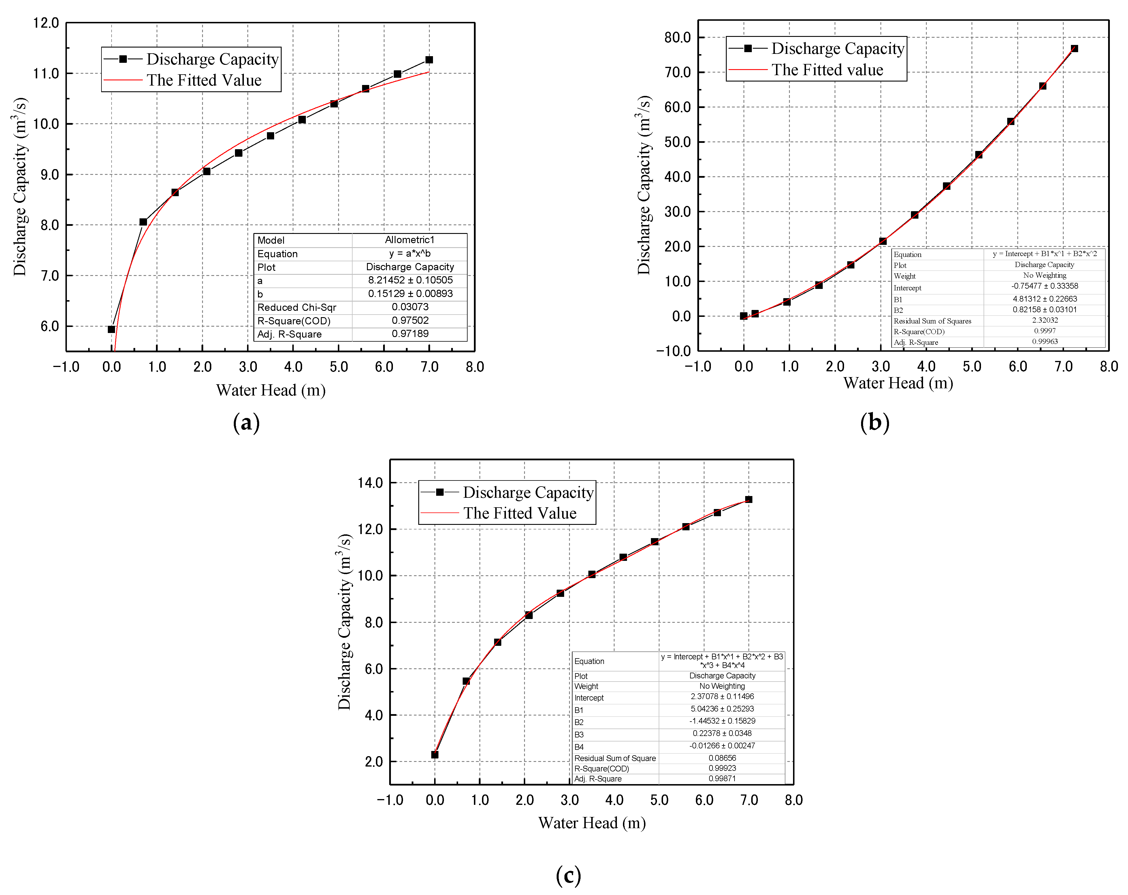
Step 5. The curve of the final discharge capacity within the well height was calculated and fitted to a function. The method to determine the final discharge curve is as follows:

At each discrete water level point, the minimum value of discharge capacity results of the free discharge, half-pressure flow and pressure flow calculated in steps 2, 3 and 4, respectively, were taken as the final discharge capacity and the calculated results were stored.

$$Q_i=\min \left\{Q_{1i},Q_{2i},Q_{3i}\right\},i=0,1,2\cdots \cdots n_{\mathrm{z}}$$

(12)

6.

Step 6. Judgment of discharge curve convergence beyond well height.

According to the fitted curve through Step 5, the water head increased at the set step size to determine the discharge capacity. $\left|Q_{\mathrm{k}+1}-Q_{\mathrm{k}}\right|<\epsilon$, $\epsilon$ serves as a convergence criterion. The discharge capacity will no longer change upon the rising of the water level. The discharge capacity beyond the convergence water level point will be a constant value.

4. Results and Discussion

The simplified algorithms were adopted to calculate the process of the water head-discharge capacity of the physical model displayed in Figure 1, and the results were fitted, as shown in Figure 4.

Based on those fitted results, the water level elevation was gradually increased in a water level step size of 0.1 m. Then, the resulting curve on the water level-discharge capacity process and the calculation error compared with the accurate algorithm method in the free discharge stage were shown in Figure 5 and Figure 6.

The calculation error of Figure 6 represents the difference between the results of an accurate algorithm method and the results of the simplified method, which was calculated according to Equation (13):

$$E_r=\frac{\left|Q^{\prime }-Q\right|}{Q}\cdot 100\%$$

(13)

where $Q$ represents the discharge capacity calculated by the accurate algorithm listed in Equations (1)–(3) for free flow, half-pressure flow and pressure flow, respectively, m³/s; $Q^{\prime }$ represents the discharge capacity calculated by the simplified method listed in Equation (5) (or Equation (6)), Equations (10) and (11) for free flow, half-pressure flow and pressure flow, respectively, m³/s.

The statistical data on calculation errors between the simplified and accurate algorithms are displayed in

Table 2. Statistical table on errors in both simplified and accurate algorithms in the free discharge stage.

Water Level (m)	Discharge Capacity from the Accurate Algorithm (m3/s)	Discharge Capacity from Simplification-Fitting Algorithm (m3/s)	Error (%)	Average Error (%)
400.5	1.60	1.86	15.80
401.5	7.70	8.31	8.01
402.5	16.04	16.41	2.31
403.5	26.34	26.16	0.69	4.19
404.5	37.94	37.54	1.06
405.5	51.30	50.57	1.42
406.5	65.30	65.24	0.08

. According to the calculation results, the average error in the simplified algorithm is +4.19% as compared with the accurate algorithm. Errors in the early discharge stage are significant, with a maximum error of +15.8%. However, the discharge capacity is generally small in the early stage. The resulting difference inflow has little influence on the holistic process of flood routing. In the later period, as the water level rises, the calculation accuracy gradually improves and has relatively high overall accuracy.

Based on the fitted results, the water level is gradually increased in a water level step size of 0.1 m. The discharge capacity on each water level was calculated based on fitted results and compared with those calculated by the accurate algorithm. The resulting curve on the water level-discharge capacity process is shown in Figure 7, and the calculation errors compared with the accurate algorithm method calculated by Equation (12) in the half-pressure flow stage are shown in Figure 8.

The statistical data on the calculation errors between the “simplification-fitting” algorithm and the accurate algorithm are displayed in

Table 3. Statistical table on errors between the simplified and accurate algorithms in the half-pressure flow stage.

Water Level (m)	Discharge Capacity from the Accurate Algorithm (m3/s)	Discharge Capacity from Simplification-Fitting Algorithm (m3/s)	Error (%)	Average Error (%)
400.5	4.04	4.19	3.52
401.5	6.79	7.00	3.20
402.5	8.52	8.57	0.57
403.5	9.75	9.63	1.22	1.87
404.5	10.83	10.61	2.07
405.5	11.78	11.63	1.34
406.5	12.66	12.50	1.21

. According to the calculation results above, the average error in the “simplification-fitting” algorithm is +1.87%, as compared with the accurate algorithm. The error is large in the early stage of half-pressure flow. However, in light of the entire discharge process, the early stage belongs to the free discharge so the results from the simplified algorithm of half-pressure flow in the early stage will not be adopted; therefore, errors arising from this stage can be ignored.

Based on those fitted results, the water level elevation is gradually increased in a water level step size of 0.1 m. The discharge capacity on each water level was calculated based on fitted results and compared with those calculated by the accurate algorithm. Then, the resulting curve on the water level-discharge capacity process is shown in Figure 9, and the calculation errors compared with the accurate algorithm method calculated by Equation (12) in the pressure flow stage are shown in Figure 10.

The statistical data on calculation errors between the “simplification-fitting” algorithm and the accurate algorithm are displayed in

Table 4. Statistical table on errors between the simplified and accurate algorithms in the pressure flow stage.

Water Level (m)	Discharge Capacity from the Accurate Algorithm (m3/s)	Discharge Capacity from Simplification-Fitting Algorithm (m3/s)	Error (%)	Average Error (%)
400.5	7.44	7.22	2.91
401.5	8.53	8.66	1.59
402.5	9.14	9.23	0.97
403.5	9.64	9.56	0.86	1.23
404.5	10.10	9.98	1.21
405.5	10.54	10.56	0.17
406.5	10.96	11.06	0.89

. According to the calculation results, the average error in the simplified algorithm is +1.23%, as compared with the accurate algorithm. The error is large in the early stage. However, in light of the entire discharge process, the early stage belongs to the free discharge; therefore, the results from the simplified algorithm of pressure flow in the early stage will not be adopted; thus, errors arising from this stage can be ignored.

In terms of the determination of the curve on the final discharge capacity within the well height, $Q_i=\min \left\{Q_{1i},Q_{2i},Q_{3i}\right\},i=0,1,2\cdots \cdots n_{\mathrm{z}}$, the results on the final discharge capacity within well height in this example are displayed in

Table 5. Table on results of final discharge capacity within well height.

Water Level (m)	Discharge Capacity (m3/s)
400.5	1.86
401.5	7.00
402.5	8.57
403.5	9.56
404.5	9.98
405.5	10.56
406.5	11.06

.

According to the determined convergence criterion $\left|Q_{\mathrm{k}+1}-Q_{\mathrm{k}}\right|<\epsilon$, $\epsilon$ is the convergence criterion. The convergence criterion should match the distance between the discrete water level points. In this example, $\epsilon$ = 0.50. Therefore, the discharge capacity converged when the water level reached 406.5 m. Thus, in terms of water level above 406.5 m, a constant discharge capacity of 11.06 m³/s should be the maximum discharge capacity value of this flood-discharging system.

5. Conclusions

This paper derived a “simplification-fitting” calculation method for window-type draining wells of a tailing pond. Several conclusions can be drawn:

• The “simplification-fitting” algorithm, together with the mathematical fitting method introduced, facilitated the expression of calculation formula for discharge capacity;
• The mathematical relationship existing in the discharge capacity between windows was deduced, thus the discharge capacity at the rest of the discrete points can be directly deduced once the discharge capacity at the first discrete point is known, and the calculation step of orifice flow can be omitted;
• Due to the unique discrete method concerning the water level, the parameters related to the water level in empirical calculation formulas under half-pressure flow and pressure flow were simplified;
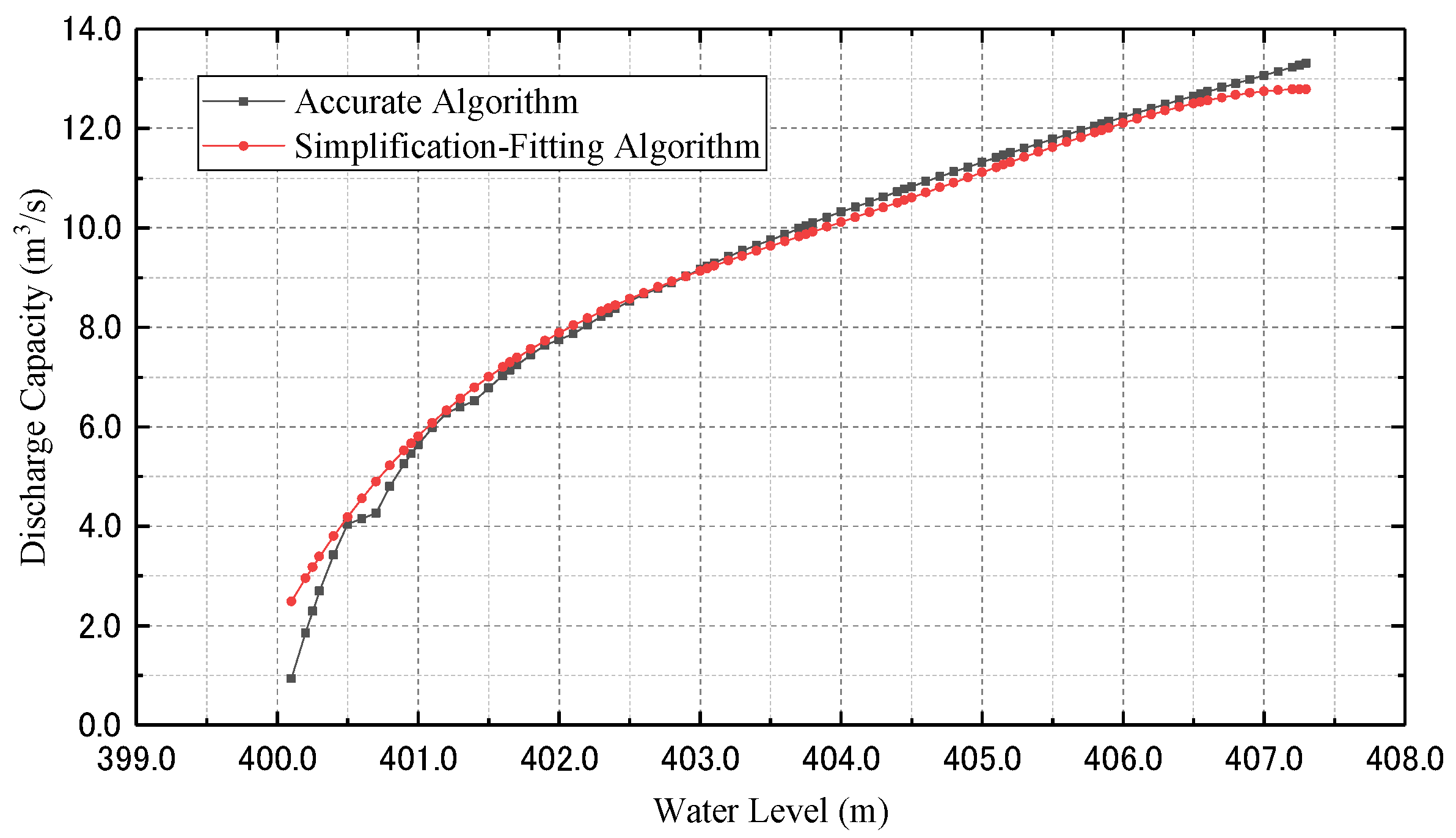
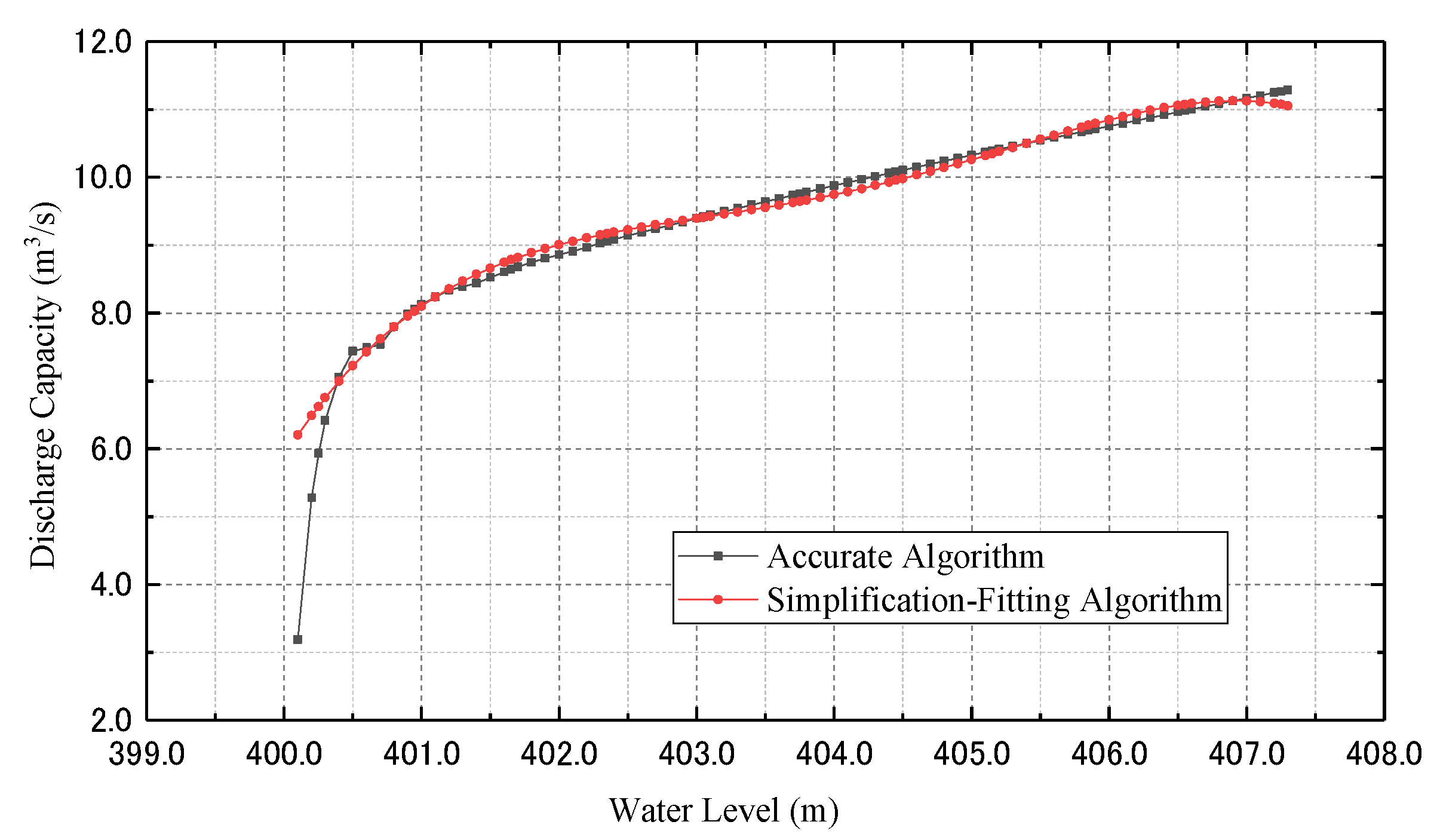
• The final discharge capacity curve adopted the minimum value among the free flow, half-pressure flow and pressure flow on each water level step and thus avoided the difficulty in calculating the intersection point among the three discharge capacity curves;
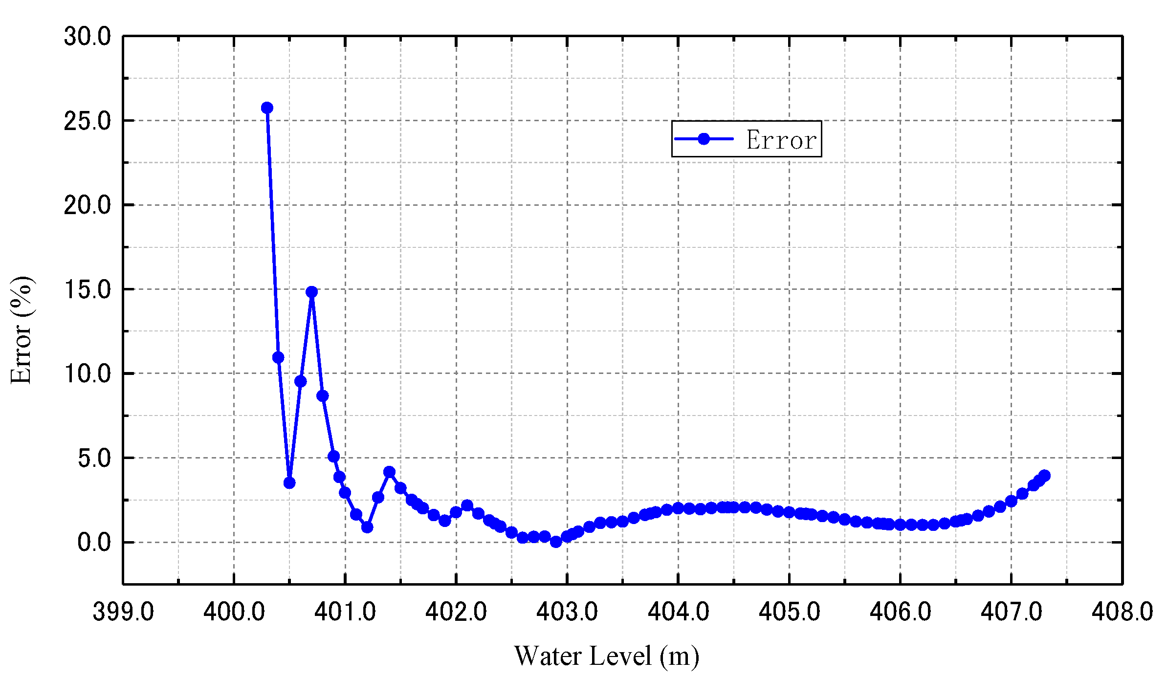
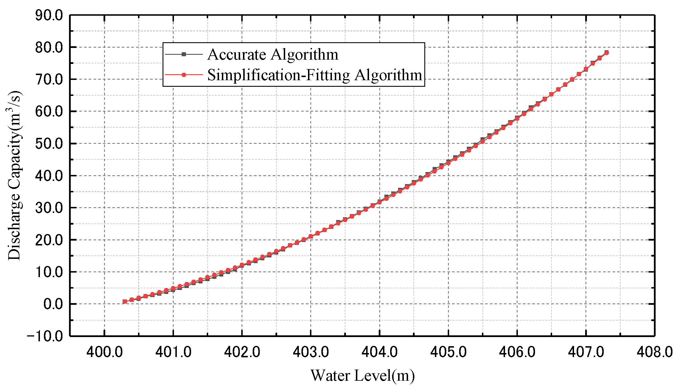
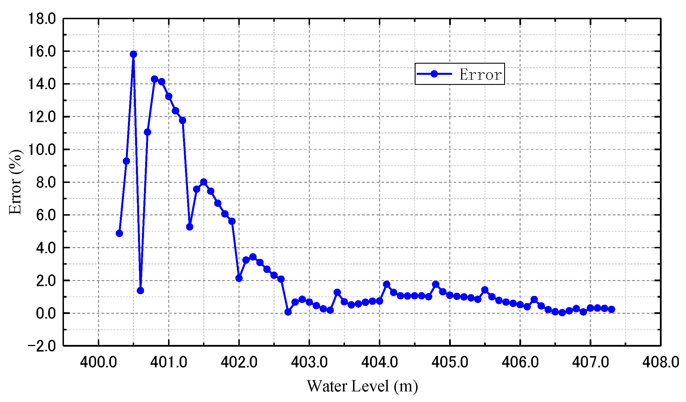
• The average error in the “simplification-fitting” algorithm compared with the accurate algorithm for free flow, half-pressure and pressure flow stage is +4.91%, +1.87%, +1.23%, respectively.

The presented study refers to the simplification of a calculation method in a flood discharge system for a tailing pond. According to the empirical formulas, discharge capacity and water level are bonded by a complicated non-linear relationship, During the process of developing a flood routing system, if the discharge capacity under three flow regimes is calculated in strict accordance with the theoretical calculation formula, not only is it challenging to locate the intersection points of three discharge curves, but also formulas will grow complicated and parameters must be constantly changed, which will result in difficulties in terms of computer programming. The simplified method proposed in this study can meet the accuracy and efficiency requirements of automatic discharge capacity calculation by the flood-discharging system.

References

1. Clarkson, L.; Williams, D. An Overview of Conventional tailing Dam Geotechnical Failure Mechanisms. Min. Metall. Explor. 2021, 38, 1305–1328. [Google Scholar] [CrossRef]
2. Koppe, J.C. Lessons Learned from the Two Major tailing Dam Accidents in Brazil. Mine Water Environ. 2021, 40, 166–173. [Google Scholar] [CrossRef]
3. Shahriari, M.; Aydin, M.E. Lessons learned from analysis of Los Frailes tailing dam failure. In Proceedings of the International Conference on Applied Human Factors and Ergonomics, San Diego, CA, USA, 16–20 July 2017; Springer: Cham, Switzerland, 2017; pp. 309–317. [Google Scholar]
4. Marti, J.; Riera, F.; Martínez, F. Interpretation of the Failure of the Aznalcóllar (Spain) tailing Dam. Mine Water Environ. 2020, 40, 189–208. [Google Scholar] [CrossRef]
5. Zhou, Z.G.; Li, P.; Guo, R. Reliability Analysis on Flood Control Capacity of Drainage System of a Certain tailing Pond in Huanren. Min. Eng. 2016, 14, 52–54. [Google Scholar]
6. Li, B.H.; Diao, M.J.; Yang, H.B. Hydraulic calculation of drainage system of tailing ponds. J. Southwest Univ. Natl. Nat. Sci. Ed. 2007, 33, 613–617. [Google Scholar]
7. Li, Y.H.; Dai, C.J. Discussion on discharge capacity calculations of drainage system of tailing ponds. Heilongjiang Metall. 2009, 29, 26–29. [Google Scholar]
8. Tan, J.J. Discharge capacity analysis of a tailing pond after drainage system combined. Mod. Min. 2016, 7, 220–221. [Google Scholar]
9. Liu, X.L.; Zhang, P.H.; Wang, X. Hydraulic Characteristic Research of Longtan Reservoir Spillway Diversion Tunnel. J. Water Resour. Archit. Eng. 2015, 13, 4. [Google Scholar]
10. Wang, Y.Y.; She, C.X.; Chen, Y.Q.; Chen, J.Y.; Jia, P.; Yin, Z.Q.; Li, Y.; Jin, J.C. Influence of Shaft Depth on Discharge Capacity of tailing Pond Flood System. J. Water Resour. Archit. Eng. 2017, 15, 133–137, 205. [Google Scholar]
11. Han, C. Hydraulic Model Test and Hydraulic Calculation of Tailing Pond Drainage System. Master’s Thesis, Shijiazhuang Tiedao University, Shijiazhuang, China, 2017. [Google Scholar]
12. Du, Z.F.; Wu, W.W.; Wu, Y.G. Hydraulic Model Test of Flood Discharge System of a Large tailing Reservoir. Nonferrous Met. Min. Sect. 2019, 71, 64–71. [Google Scholar]
13. Djillali, K.; Abderrezak, B.; Petrovic, G.A.; Sourenevan, B.E. Discharge capacity of shaft spillway with a polygonal section: A case study of Djedra dam (East Algeria). Water Sci. Technol. Water Supply 2021, 21, 1202–1215. [Google Scholar] [CrossRef]
14. Fraga, I.; Cea, L.; Puertas, J. Validation of a 1D-2D dual drainage model under unsteady part-full and surcharged sewer conditions. Urban Water J. 2017, 14, 74–84. [Google Scholar] [CrossRef]
15. Zakwan, M.; Khan, I. Estimation of Discharge coefficient for side weirs. Water Energy Int. 2020, 62, 71–74. [Google Scholar]
16. Ebtehaj, I.; Bonakdari, H.; Gharabaghi, B. Development of more accurate discharge coefficient prediction equations for rectangular side weirs using adaptive neuro-fuzzy inference system and generalized group method of data handling. Measurement 2018, 116, 473–482. [Google Scholar] [CrossRef]
17. Sen, S. Surface pressure and viscous forces on inclined elliptic cylinders in steady flow. Sādhanā 2020, 45, 172. [Google Scholar] [CrossRef]
18. Dennis, S.C.R.; Young, P.J.S. Steady flow past an elliptic cylinder inclined to the stream. J. Eng. Math 2003, 47, 101–120. [Google Scholar] [CrossRef]
19. Mo, S.J. Numerical Simulation of Hydraulic Characteristics of Tailing Pond. Master’s Thesis, Shijiazhuang Tiedao University, Shijiazhuang, China, 2016. [Google Scholar]
20. Zhao, J.Y. The Hydraulic Characteristic Research for Volute. Master’s Thesis, Northwest A & F University, Xianyang, China, 2017. [Google Scholar]
21. Bao, Z.J.; Wang, Y.H. Three-Dimensional Numerical Simulation of Spillway Based on Flow—3D. Zhejiang Hydrotech. 2012, 2, 5–9. [Google Scholar]
22. Wang, Y.H.; Bao, Z.J.; Wang, B. Three-dimensional Numerical Simulation of Flow in Stilling Basin based on Flow-3D. Eng. J. Wuhan Univ. 2012, 45, 454–457, 476. [Google Scholar]
23. Ling, L.; Chen, R.C.; Li, Y.H. Three-dimensional VOF Model and its Application to the Water Flow Calculation in the Spilway. J. Hydroelectr. Eng. 2007, 26, 83–87. [Google Scholar]
24. Yi, C. Numerical Simulation of Hydraulic Characteristics of Tailing Pond. Master’s Thesis, Nanchang University, Nanchang, China, 2016. [Google Scholar]
25. Yu, K.; Cheng, Y.; Zhang, X. Hydraulic characteristics of a siphon-shaped overflow tower in a long water conveyance system: CFD simulation and analysis. J. Hydrodyn. 2016, 28, 564–575. [Google Scholar] [CrossRef]
26. He, M.M. Discussion on Hydraulic Model Test and Numerical Simulation of tailing Pond Drainage System. Constr. Decor. 2021, 7, 48. [Google Scholar]
27. Wang, S.X. Discharge Capacity of Shaft Spillway with Framed Inlettower for High tailing Dam. Met. Mine 1994, 5, 36–39,47. [Google Scholar]
28. Wu, G.G.; Liu, X.F.; Lu, J.J.; Shen, L.Y. Comparison of Two Hydraulic Calculation Methods for Drainage System of tailing Pond. Nonferrous Met. Eng. Res. 2011, 32, 6–8. [Google Scholar]
29. Ning, F.; Li, X.U. Application of GMRES Algorithm in the Predictions of Two-Dimensional Inviscous Steady Flows. Chin. J. Comput. Phys. 2001, 33, 442–451. [Google Scholar]
30. Liu, C. Discussion on Flow Capacity of Chute Flood Drainage System in tailing Pond. Ment. Mine 2012, 1, 15–18. [Google Scholar]
31. Dang, N. Tailing Drainage Wells Experimental Study on Shape Optimization of Flood Discharge System. Master’s Thesis, Xi’an University of Technology, Xi’an, China, 2010. [Google Scholar]
32. Shi, W. Discussion on Flood Discharge System Design of tailing Pond. Nonferrous Mines 2002, 31, 43–46. [Google Scholar]
33. Yu, D.X. Design and Optimization Method of Flood Discharge System in tailing Reservoir. China Met. Bull. 2018, 268–269. [Google Scholar]
34. Shang, X.J.; Su, X.L. Design and Optimization Method of Flood Discharge System in tailing Reservoir. Hydroelectr. Sci. Tecnol. 2019, 2, 90–91. [Google Scholar]
35. Yang, M.J. Study on Optimization Technology of flood discharge system of a tailing pond. World Nonferrous Met. 2020, 9, 273–274. [Google Scholar]
36. Zhang, C.H. Software Development and Engineering Application of the Tailing Dam Complex Flood Drainage. Master’s Thesis, Shijiazhuang Tiedao University, Shijiazhuang, China, 2015. [Google Scholar]
37. Ma, W.J. Software Development and Application of HydraulicCalculation of the Tailing Dam Drainage System. Master’s Thesis, Shijiazhuang Tiedao University, Shijiazhuang, China, 2014. [Google Scholar]
38. Chen, H.; Li, R.L.; Jia, Y.; Wang, J.R. Discussion on calculation method of discharge capacity of drainage system. Mod. Min. 2015, 31, 180–183. [Google Scholar]
39. Reference Materials for Tailing Facility Design Writing Group. Reference Materials for Tailing Facility Design; Metallurgical lndustry Press: Beijing, China, 1980; pp. 621–628. [Google Scholar]
Figure 1. A window-type draining system in a tailing pond.
Energies 15 04194 g001
Figure 2. Flow chart of the simplified algorithm for discharge capacity of window-type draining wells.
Energies 15 04194 g002
Figure 3. Water level discrete method.
Energies 15 04194 g003
Figure 4. Fitted value of results calculated through simplified algorithm for discharge capacity: (a) free flow; (b) half-pressure flow; and (c) pressure flow.
Energies 15 04194 g004
Figure 5. Figure on discharge capacity results from both simplified and accurate algorithms in the free discharge stage.
Energies 15 04194 g005
Figure 6. Figure on the errors of simplified and accurate algorithms in the free flow stage.
Energies 15 04194 g006
Figure 7. Figure on discharge capacity results from both simplified and accurate algorithms in the half-pressure flow stage.
Energies 15 04194 g007
Figure 8. Figure on errors of simplified and accurate algorithms in the half-pressure flow stage.
Energies 15 04194 g008
Figure 9. Figure on discharge capacity results from both simplified and accurate algorithms in the pressure flow stage.
Energies 15 04194 g009
Figure 10. Figure on errors of simplified and accurate algorithms in the pressure flow stage.
Energies 15 04194 g010